Modern Economy
Vol.5 No.8(2014), Article
ID:47917,8
pages
DOI:10.4236/me.2014.58080
Does the Implied Volatility Index Have Signaling Power? Evidence from Mexico
Jin Yong Yang1, Junyoung Heo2, In-Sung Yeo3, Sang-Heon Lee4
1Hankuk University of Foreign Studies, Seoul, South Korea
2Hansung University, Seoul, South Korea
3Seoul National University, Seoul, South Korea
4Hanyang University, Seoul, South Korea
Email: jyang0112@gmail.com, jyheo@hansung.ac.kr, pros53@snu.ac.kr, paco@hanyang.ac.kr
Copyright © 2014 by authors and Scientific Research Publishing Inc.
This work is licensed under the Creative Commons Attribution International License (CC BY).
http://creativecommons.org/licenses/by/4.0/


Received 22 May 2014; revised 18 June 2014; accepted 11 July 2014
ABSTRACT
This paper investigates whether the implied volatility index has signaling power for the future stock index returns from VIMEX (Mexican Implied Volatility Index) and MEXBOL (Mexican BOLSA IPC Index) and if there was a change in signaling power between, before, and after the international financial crisis. We find that the implied volatility index is a meaningful indicator and that its signaling power changes between pre and post crisis. In the post crisis period, the VIMEX still works as a meaningful indicator, but the predictive power is weakened compared to the previous period. Finally, we implemented a trading strategy using the VIMEX signal to test the quality of the signal. Our results show that the VIMEX driven strategy returns outperform the benchmark returns of the outright long MEXBOL position.
Keywords:Implied Volatility, VIMEX, Expected Returns

1. Introduction
Traders and investors look at and measure volatility in a number of different ways which include historic volatility, realized volatility, and expected volatility among others. “Implied volatility” refers to volatility that explains the market price of options which are measured in the option pricing formula. Volatility indices have been introduced on the basis of the implied volatilities in specific classes of options and a great deal of attention has been taken on their properties. The first market volatility index was the VIX introduced by the CBOE in 1993.
The VIX is a forward-looking volatility that investors can expect. The VIX is known to have a negative correlation with stock index returns. It is also known to be an indicator of the market’s sentiment and investors’ fear. Sometimes the VIX is used for asset allocation by investment firms. The S&P 500 provided a positive total return after the VIX reached extremely high levels. Furthermore, with a more frequent positive return, the VIX level becomes more extreme1. The VIX is range-bound and reversion tends to occur at upside and downside extremes.
The volatility level can be a market signal to indicate future bullishness or bearishness in the stock market, viz., low volatility is a bearish signal while high volatility indicates a rally. This is an idea used by a contrarian. Prolonged or extremely high volatility means “fear”, anxiety or even panic, which can be recognized as a bullish indicator because the weak hands have already been shaken out. Prolonged or extremely low volatility means “complacency”, which can be regarded as a bearish precursor because markets may falter.
This belief has two bases, viz., statistical and theoretical. A statistical basis is affirmed by assessing the statistical significance between the volatility level and the future stock returns. A theoretical basis is identified by finding out along which channels the implied volatility levels are connected with the future stock returns [1] . The behavior of the implied volatility has attracted researchers’ interest2.
Alessandro Cipollinni and Antonio Manzini [1] provided an answer to the statistical issue by adopting the procedure of Campbell and Shiller [2] 3 and of Giot [3] 4. Their research indicates that the VIX can signal market direction. The signal is loud and clear when the implied volatility is high (or, even better, when it spikes). Prithviraj S. Banerjee, James S. Doran, David R. Peterson [4] found that the VIX variables significantly affect returns for most portfolios, with the relationship being stronger for high beta portfolios. Variable levels and innovations are important. Yakup Eser Arisoy, Aslihan Salih, Levent Akdeniz [5] suggested that volatility risk explains a significant amount of variation in securities returns, especially during high-volatility periods.
In the way of Whaley [6] , the relation between the VIX and SPX is asymmetric, so the VIX is an investors’ fear gauge in a market fall rather than an investors’ excitement gauge in a market rally. As a contrarian indicator, VIX is more relevant at market bottom5. Ralf Becker, Adam E. Clements and Andrew McClelland [7] considered two issues relating to the information content of the VIX6. Silmai [8] investigated the information spillover between VIX changes and SPX returns. N. Bada and Y. Sakurai [9] investigated whether macroeconomic variables can predict the regime switches in the VIX index7. Jianhua Gang and Xiang Li [10] used the bivariate semi-nonparametric (SNP) model by Gallant and Tauchen [11] to study the contemporaneous relationship between the innovation of VIX and the expected SPX returns8. Ghulam Sarwar [12] have examined whether the relation between stock market returns and VIX has changed over time9. Kozyra and Lento [13] provided an insight into the relation between the VIX and technical analysis10.
In this paper, we examine if the implied volatility index can signal market direction from VIMEX and MEXBOL. The rest of this paper is organized as follows. Section 2 details the methodology implemented and contains the data description. Section 3 presents and interprets the results. Section 4 shows a VIMEX timing strategy driven by the VIMEX signal. Finally, Section 5 concludes with remarks.
2. Methodology and Data
To find out if implied volatility might have reliable signaling power, we test the correlation of the VIMEX relative level to subsequent moves in the MEXBOL index. “Relative level” is defined as the ratio of the VIMEX to its own N-day moving average minus one (e.g. if VIMEX = 20, N-day MA = 16, then Relative level = (20/16) − 1 = 25%). The MEXBOL return was taken from the VIMEX close to K days out.
We employ daily data from March 26, 2004 to Aug 6, 2012 (2084 observations). The variables observed are the VIMEX and the MEXBOL series. The dataset is divided into two periods: before the bankruptcy of Lehman Brothers (26/03/2004-12/09/2008, 1114 observations), and after the bankruptcy of Lehman Brothers (13/09/ 2008-06/08/2012, 970 observations).
3. Empirical Results and Interpretation
Figure 1 shows that the level of the VIMEX tended to rise when the MEXBOL dropped. The VIMEX has spiked during the period of market turmoil, whereas it has fallen dramatically with the rally of MEXBOL. The market’s rally tends to continue during the period of low VIMEX, and the VIMEX rises faster than it falls. The VIMEX has a negative correlation with the MEXBOL.
In the period of pre-crisis (see Figure 2), the highest degree of linear predictive power occurred using a 188 trading day moving average for the VIMEX, predicting 63 trading days out on the MEXBOL. But the results have still been strong for the lower values of K and N.
Even though short predictive periods—viz. low K—are less effective, it can be counterbalanced by the increased number of trading opportunities because both short and longer periods indicate the same direction. The trading strategies using only a 4-day period also can obtain good results.
The scatter diagram of the raw divergence from the MA vs. returns for the predictive peak N = 188, K = 63 provides important implications (see Figure 3). It shows that the relationship of the two is more linear at the higher relative VIMEX (the greater divergence from the MA), and the VIMEX is a better signal of 63-day rallies than of selloffs. We find that high relative VIMEX is a significant signal which is valuable as a timing indicator.
Table 1 represents the regression results of MEXBOL return on relative VIMEX before the crisis.
In the period of Post crisis, the VIMEX still works as a meaningful indicator. There is a predictive peak at N = 250, K = 59, but it slightly reduces the correlation between relative VIMEX and MEXBOL returns (see Figure 4). In other words, the predictive power is weakened slightly compared to the previous period11.
As shown in the scatter diagram, high relative VIMEX is still the most significant signal. On the other hand, a great number of points are clustered disorderedly around relative VIMEX levels of 0% to −10% (see Figure 5). That is, when the VIMEX is measured a little below MA, the MEXBOL returns are erratic rather than falling as common sense predicts12. Nevertheless, it is also evident that the largest fall in the MEXBOL returns tend to occur when the relative VIMEX is low. And the MEXBOL returns’ sharp drops hardly occur in the high relative VIMEX environment.
Table 2 represents the regression results of MEXBOL return on relative VIMEX after the crisis.
Since the MEXBOL returns move dispersedly in the low relative VIMEX and low VIMEX is an obvious indicator of low option prices, those are opportune times to buy both puts and calls, viz. straddle. The relative VIMEX works as a directional signal, but it is also possible to use options to take advantage of arbitrary dispersion of the MEXBOL returns that occur during the low relative VIMEX environment.
Instead of a predictive peak, maximizing returns from the VIMEX strategy shows different parameters for N

Table 1 . Regression of MEXBOL return on relative VIMEX (Pre Crisis 2004/03/26-2008/09/12).
Table 2. Regression of MEXBOL return on relative VIMEX (After Crisis 2008/09/13-2012/02/07).
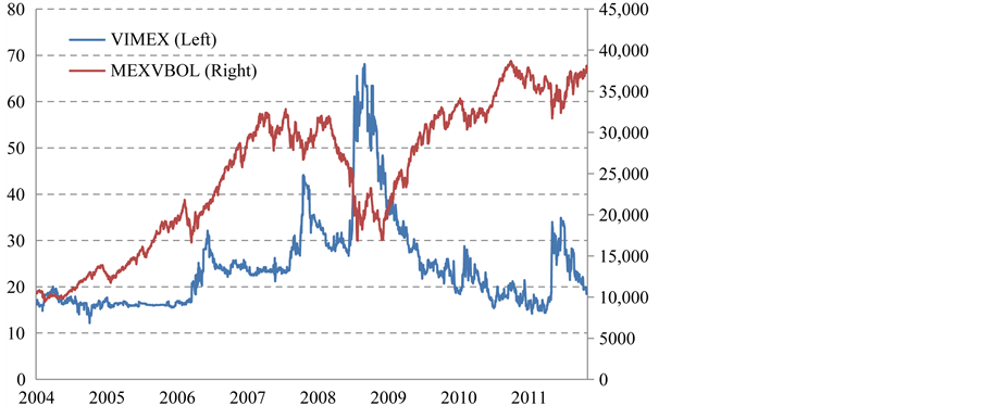
Figure 1. MEXBOL (Mexican Stock Index) vs. VIMEX (Mexican VIX).
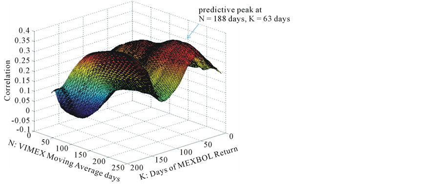
Figure 2. Correlation of VIMEX level relative to N-day moving average vs. subsequent K-day MEXBOL return (Pre Crisis 2004/03/26-2008/09/12).
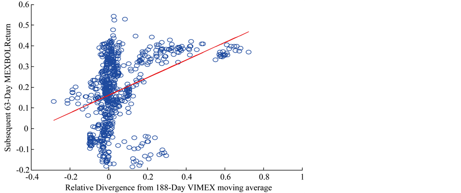
Figure 3. Relative divergence from 188-day VIMEX moving average vs. subsequent 63-day MEXBOL return (Pre Crisis 2004/03/26-2008/09/12).
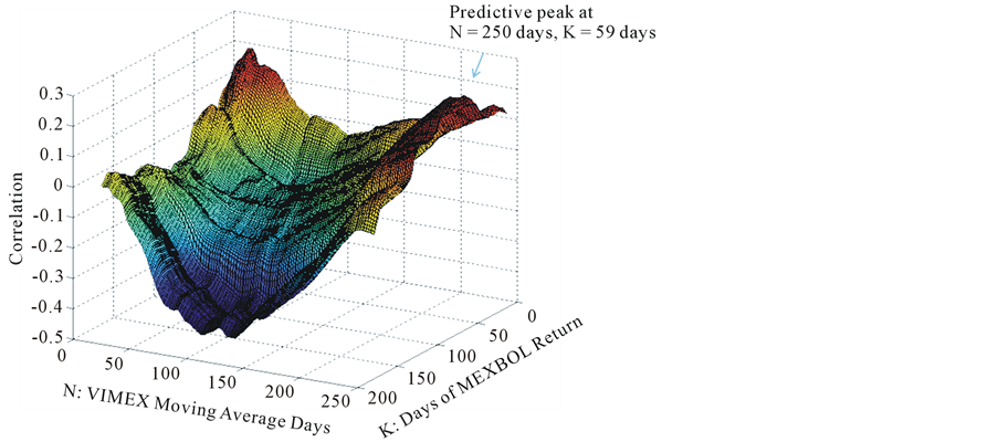
Figure 4. Correlation of VIMEX level relative to N-day moving average vs. subsequent K-day MEXBOL return (After Crisis 2008/09/13-2012/02/07).

Figure 5. Relative divergence from 250-day VIMEX moving average vs. subsequent 59-day MEXBOL return (After Crisis 2008/09/13-2012/02/07).
and K. Our VIMEX strategy consists in opening a K-days buy-and-hold position on the MEXBOL whenever relative VIMEX to N-day MA is greater than 5%. In this case, N is 20-day and K is 25 days before crisis, whereas N = 20, K = 14 after crisis. The averaging period N is equal, but the holding period K is shortened after the crisis.
4. A VIMEX Timing Strategy Driven by the VIMEX Signal
A VIMEX timing strategy used in the back test is simply to take a long or short position in a size proportional to the ratio of VIMEX to its MA; if VIMEX is above the N-day MA, buy and hold K days, if VIMEX is below the N-day moving average, short-sell K days. This strategy can be understood intuitively; if VIMEX is above (below) the N-day MA, the market price falls (rises), to deviate from the intrinsic value by fear (by relief), so buy (sell) and wait until the recovery of the intrinsic value, to repeat it, pursue a statistically significant profit.
In the VIMEX timing strategy, the investor determines “buy” or “sell” based on the information of N days, and then holds K days. Because the investors make investment decisions as described above in each trading day, the investors have K portfolios which are different by one day at the composition time. R(N, K) is the rate of return on the investment in equal proportion to the K portfolios13.
When the investment signal, “s”, is
![]() the weight of investment, “w”, is proportional to “s”.
the weight of investment, “w”, is proportional to “s”.
![]()
When the investor invests “w” in the VIMEX timing strategy and “1 − w” in the risk-free rate of return, the rate of return of the day is as follows:

The excess rate of return is  obtained by subtracting “r” from the total return. Then, Sharpe ratios are calculated as follows:

The proportionality constant γ, since it is cleared by the formula Sharpe ratio, need not be estimated here. We find N, K to have a maximum Sharpe ratio for the total period, to place 2 - 250 to N, 1 - 20 to K. As a result, we get N = 7, K = 3, annualized Sharpe ratio = 0.53914. It means that N and K are shortened to maximize the Sharpe ratio instead of linear signaling power. Optimizing the signal’s time horizons, we find the best risk/return with a short N, K.
When the initial asset is 1, the final asset value is:

Therefore, when N, K is determined, the final asset value is a function of γ. The γ, is an index that shows how to trust the investment signal, ![]() to maximize,
to maximize, ![]() can be interpreted as a kind of Kelly ratio that maximizes the long-term growth rate. The final asset value is illustrated by the following, when γ is changed from 0 to 100 for the specified variable:
can be interpreted as a kind of Kelly ratio that maximizes the long-term growth rate. The final asset value is illustrated by the following, when γ is changed from 0 to 100 for the specified variable:
As Figure 6 shows, it is confirmed that at γ = 44.3, the value is maximized to 5.0876. We try to run the VIMEX timing strategy for (N, K, γ) = (7, 3, 44.3). Figure 7 and Figure 8 represent the signal strength before and after crisis as follows.
For the benchmark, we use an outright long MEXBOL position in a size equal to the RMS average15 of the test strategy’s position size. The cumulative return of the test strategy beat the benchmark in the long term (see Figure 9). The performance of the test strategy is improved further if the investor holds only risk-free assets at the time of having an extremely large value, such as the event of a financial crisis, e.g. Lehman shock in 2008, Europe crisis in 2011.
When the VIMEX increases extremely over the moving average, as in the financial crisis, the investor can be exposed to a big loss by bulk buying because the increase in the VIMEX due to the financial crisis indicates a fall further in the future. In this case, the VIMEX timing strategy may serve to amplify a sort of tail risk16. By improved strategy, it is possible to avoid an unexpected loss and earn more than nine times the initial asset value during the test period (see Figure 10).
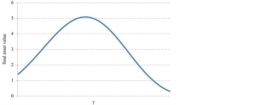
Figure 6. The changes in final asset value by γ.
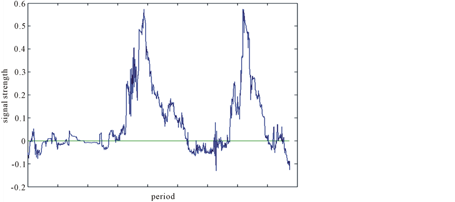
Figure 7. Signal strength before crisis.
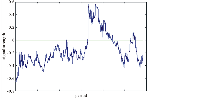
Figure 8. Signal strength after crisis.
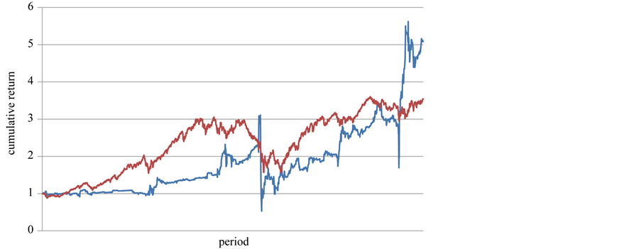
Figure 9. Cumulative return on VIMEX timing strategy (blue) vs. Normalized MEXBOL total return (red).
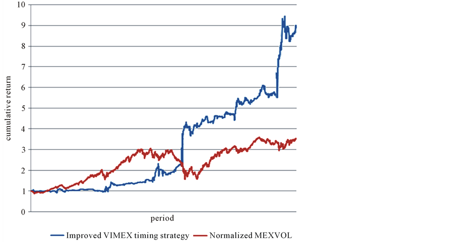
Figure 10. Cumulative return on Improved VIMEX timing strategy (blue) vs. Normalized MEXBOL total return (red).
5. Concluding Remarks
In this paper, we have investigated whether an implied volatility index could signal market direction. Is an implied volatility index a meaningful indicator? Our answer is “Yes”. But we have found that its signaling power changed to a certain extent before and after the international financial crisis with stronger signaling before the crisis, and slightly weaker signaling after the crisis. In reality, an implied volatility index works differently as a directional signal depending on the state of the market, since it is related to behavioral parameters.
Finally, the market timing strategy using the VIMEX signal outperforms the simple strategy of the outright long MEXBOL position. The VIMEX timing strategy has a higher return and lower volatility resulting in a higher Sharpe ratio. This may facilitate the trading strategy increasing alpha with the VIMEX, as an independent source of alpha17.
Acknowledgements
This research was financially supported by Hansung University.
References
- Cipollini, A.P.L. and Manzini, A. (2007) Can the VIX Signal Market’s Direction? An Asymmetric Dynamic Strategy. Social Science Research Network (SSRN).
- Campbell, J.Y. and Shiller, R.J. (1998) Valuation Ratios and the Long-Run Stock Market Outlook. Journal of Portfolio Management, 24, 11-26. http://dx.doi.org/10.3905/jpm.24.2.11
- Giot, P. (2005) Relationships between Implied Volatility Indexes and Stock Index Returns. Are Implied Volatility Indexes Leading Indicators? Journal of Portfolio Management, 31, 92-100. http://dx.doi.org/10.3905/jpm.2005.500363
- Banerjee, P.S., Doran, J.S. and Peterson, D.R. (2007) Implied Volatility and Future Portfolio Returns. Journal of Banking & Finance, 31, 3183-3199. http://dx.doi.org/10.1016/j.jbankfin.2006.12.007
- Arisoy, Y.E., Salih, A. and Akdeniz, L. (2007) Is Volatility Risk Priced in the Securities Market? Evidence from S&P 500 Index Options. Journal of Futures Markets, 27, 617-642.
http://dx.doi.org/10.1002/fut.20242 - Whaley, R.E. (2009) Understanding the VIX. The Journal of Portfolio Management, 35, 98-105. http://dx.doi.org/10.3905/JPM.2009.35.3.098
- Becker, R., Clements, A.E. and McClelland, A. (2009) The Jump Component of S&P 500 Volatility and the VIX Index. Journal of Banking & Finance, 33, 1033-1038.
http://dx.doi.org/10.1016/j.jbankfin.2008.10.015 - Simlai, P. (2010) What Drives the Implied Volatility of Index Options & Quest. Journal of Derivatives & Hedge Funds, 16, 85-99. http://dx.doi.org/10.1057/jdhf.2009.20
- Baba, N. and Sakurai, Y. (2011) Predicting Regime Switches in the VIX Index with Macroeconomic Variables. Applied Economics Letters, 18, 1415-1419.
http://dx.doi.org/10.1080/13504851.2010.539532 - Gang, J. and Li, X. (2014) Risk Perception and Equity Returns: Evidence from the SPX and VIX. Bulletin of Economic Research, 66, 20-44.
- Gallant, A.R. and Tauchen, G. (2006) SNP: A Program for Nonparametric Time Series Analysis Version 9.0 User’s Guide. http://www.aronaldg.org/
- Sarwar, G. (2010) The VIX mARKET VOLAtility Index and US Stock Index Returns. International Journal of Business Research, 10, 166-176.
- Kozyra, J. and Lento, C. (2011) Using VIX Data to Enhance Technical Trading Signals. Applied Economics Letters, 18, 1367-1370. http://dx.doi.org/10.1080/13504851.2010.539532
NOTES

1Goldman Sachs report (Rattray and Balasubramanian [2003]).
2This research has investigated the forecasting performance and information content of implied volatility, which is a market determined forecast.
3This paper shows the valuation ratios can be used to forecast stock prices.
4This research indicates a negative relation between the changes in implied volatility index and the stock index.
5Morgan Stanley report, March 27, 2002.
6First, whether it subsumes historical information on the contribution of price jumps to volatility. Second, whether the VIX reflects any incremental information relative to model-based forecasts pertaining to future jump activity.
7They find three distinct regimes in the VIX index during the 1990 to 2010 period, the regime-switching probability from the tranquil regime to the turmoil is influenced by lower term spreads.
8They conclude that the contemporaneous risk-return behavior depends not only on the sign of the risk matrices (sentiment shifts), but also on the magnitude of the change. In other words, fear or exuberance (extreme innovation of VIX) does correlate to conditional return, but the correlation is non-monotonic and hump-shaped.
9The VIX-returns relationship vary by period, suggesting that its strength depends on the mean and volatility regime of VIX.
10Both VIX and the technical analysis are forward-looking.

11Sarwar (2012) finds that the auto-correlation structure of VIX-returns differ considerably between 1992-1997 and 1998-2011.
12Sarwar (2012) suggests that the strength of VIX-returns relation depends on the mean and volatility regime of VIX. This relation is still stronger when VIX is high and more volatile.

13Jagadeesh and Titman (1993), Gatev et al. (2006) calculate the rate of return by overlapping the portfolios in the case of holding period K > 1. Jagadeesh and Titman (1993) is the first rating of momentum strategy. Gatev et al. (2006) is the paper published for the first time in a top journal, in relation to pairs trading.
14It is annualized by assuming 250 trading days for the year.
15RMS average at time ![]() (
( is the position size from 1-day to t-day).
16Kelly (2012) shows that tail risk has strong predictive power for total return of the market.

17Alpha is a risk-adjusted measure of the active return on an investment. It is the coefficient of the constant in a market model regression. The alpha coefficient indicates the return in excess of the compensation for the risk it involved.