Wireless Engineering and Technology
Vol. 4 No. 4 (2013) , Article ID: 38677 , 7 pages DOI:10.4236/wet.2013.44027
Estimation of Two-Dimensional Correction Factors for Min-Sum Decoding of Regular LDPC Code
![]()
Department of Electrical Engineering, University of Babylon, Babel, Iraq.
Email: ahmedbabel@yahoo.com
Copyright © 2013 Ahmed A. Hamad. This is an open access article distributed under the Creative Commons Attribution License, which permits unrestricted use, distribution, and reproduction in any medium, provided the original work is properly cited.
Received August 17th, 2013; revised September 21st, 2013; accepted October 6th, 2013
Keywords: LDPC Code; Sum-Product; Min-Sum; 2-D Correction Factors; Software-Defined Radio (SDR)
ABSTRACT
In this paper, two-dimensional (2-D) correction scheme is proposed to improve the performance of conventional MinSum (MS) decoding of regular low density parity check codes. The adopted algorithm to obtain the correction factors is simply based on estimating the mean square difference (MSD) between the transmitted codeword and the posteriori information of both bit and check node that produced at the MS decoder. Semi-practical tests using software-defined radio (SDR) and specific code simulations show that the proposed quasi-optimal algorithm provides a comparable error performance as Sum-Product (SP) decoding while requiring less complexity.
1. Introduction
Due to its exceptional error performance, low density parity check code (LDPC) [1] has received significant attention recently. It is adopted by many new generation communication standards, such as wireless LAN (IEEE 802.11n) [2], WiMax (IEEE 802.16e) [3] and DVB-S2 [4]. Although Sum-Product (SP) algorithm [5] provides a powerful tool for iterative decoding of LDPC codes, it requires a large hardware complexity. Sub-optimal algorithms like Min-Sum (MS) [6] can significantly reduce the hardware complexity of SP at the cost of performance degradation. In MS decoding, the complex computations at the check nodes are approximated by using simple comparison and summation operations. The sub-optimality of the MS decoding comes from the overestimation of check-to-bit and thereby, bit-to-check node messages, which lead to performance loss with respect to the SP decoding.
In many literatures like [7-11], various methods were proposed to elevate the performance degradation of the MS decoding which is considered as quasi-optimal algorithms. It has been noted that the degradation in error performance due to MS decoding can be compensated by linear post processing (normalization or offset) of the messages delivered by check and bit nodes.
In this study, a simple algorithm is presented to estimate the optimal correction factors for 2-D corrected MS decoding of regular LDPC codes. In a previous work [12], it has been shown that the error performance loss of SOVA compared to Log-MAP decoding can be compensated by scaling the a-posteriori LLR values of the information bits based on the fact that the latter is a growing estimate to the transmitted codeword, and the correction factors can be derived based on minimizing the mean-square difference (MSD) between them. A similar approach is applied to find the optimal correction factors which are utilized to scale the message passing from check to bit and bit to check nodes. Extensive simulations are carried out using the specifications of the LDPC adopted by the IEEE 802.11n standards. A significant improvement in error performance is achieved by using the modified MS decoder compared to the original one.
This paper is organized as follows. Section 2 briefly reviews the standard SP and MS decoding schemes. Section 3 presents the proposed 2-D corrected MS decoding. In Section 4, a simple SDR implementation for the modified and unmodified systems is demonstrated. Section 5 reports simulation and practical results and Section 6 concludes this paper.
2. Standard SP and MS Decoding Algorithms
The SP and its simplified version MS are soft-decision decoders which make use of the channel information. They are developed to deal with log-likelihood values (LLR) of the received signal. As proposed by [13] efficient encoding of the information bits with a reasonable complexity is achieved to produce the codeword
 . When a codeword is transmitted through an AWGN channel the binary vector
  is first mapped into a transmitted signal vector
 according to
 . The received sequence is
 , where the samples of the received signal
  are given by
 (1)
(1)
The vector  are statistically independent Gaussian random variables with zero mean and two sided power spectral density of
  . The received signals
  have to be scaled by the channel reliability
 before they deliver to the decoder. Herethe notations R and
  define the information rate and the energy per information bit. Hence,
  is the log-likelihood ratio (LLR) of bit n which is derived from the channel output
 .
.
Suppose a regular binary (N, K) LDPC code has a bipartite Tanner graph which can be defined by the sparse parity check matrix  . The set of neighbor check nodes of the bit node n is
  . While, the set of neighbor bit nodes of the check node m, is
  . The set of bits that participate in check node m except for bit n is denoted by
 . On the other hand, the notation
  refers to the set of checks in which bit n participates except for check m. For each iteration i, the decoder calculates the following variables:
•  : The LLR message of bit n which is passed from check node m to bit node n (extrinsic information).
•  : The LLR message of bit n which is passed from bit node n to check node m.
•  : The a-posteriori LLR of bit n.
The standard SP [5], [14] decoding algorithm can be summarized by the following steps.
Step 1: Initialization: set  for each m and n, maximum number of iteration to
 ,
,  and failure = 0.
Step 2: Check node update (Horizontal step): For each m, n with  = 1, compute
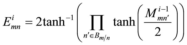 (2)
(2)
Step 3: Bit node update (vertical step): For each m, n with  = 1, compute
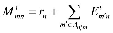 (3)
(3)
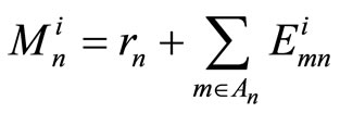 (4)
(4)
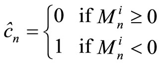
Step 3: Tentative decision: Let denote the estimated codeword bits as
If  or
or  go to step 4, otherwise set
  and go to step 2.
Step 4: Declare that  is the decoded codeword. If
  and
and  then set failure = failure + 1.
The difference between MS and SP algorithm is the way by which MS decoder computes the check node update [6]. It is recognized that the term corresponding to the smallest  dominates the product term in Equation (2) and so the product can be approximated by a minimum. Hence Equation (2) can be modified to
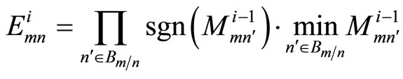 (5)
(5)
The product of sign and minimum operations are much simpler to implement and faster in time processing than the product of hyperbolic tan and its inverse. These advantages spot a light on the MS decoding algorithm and make it more feasible and preferable in practical implementations.
3. Proposed Corrected MS Decoder
Although the MS algorithm greatly reduces the decoding complexity for implementation, it suffers from a significant deterioration in its error performance compared to SP decoding. Many researches state that the correlation of the extrinsic information with the original a priori bit LLR (rn) is what prevents the resulting a-posteriori probabilities from being exact. In line with the foundation that explored in [12], it is suggested that we scale the marginal LLR values  and
and  by the correction factors ai and bi to make the a-posteriori probabilities as close as possible from the transmitted codeword, thereby reducing the probability of error. The corrected values
  and
and  are given by the following equations:
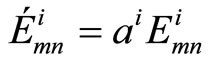 (6)
(6)
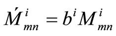 (7)
(7)
It is possible to derive the correction factor  by minimizing the mean square difference
  between the a-posteriori probability
  and the mapped codeword q. Assume that
  , then
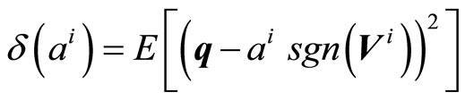 (8)
(8)
 denotes the expected value.
  may be considered as a measure of how efficient the algorithm is with the proposed modification. It is obvious that to get better suboptimal decoding, the parameter
  should be found to minimize
  . The value of
  is simply found by derive
  with respect to
  and equating the result to zero.
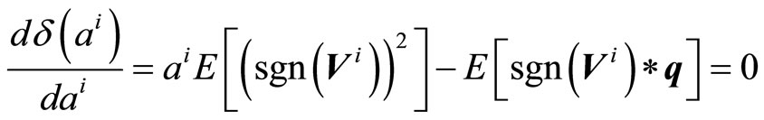 (9)
(9)
Considering that 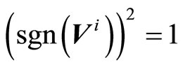 , the value of
  is given by
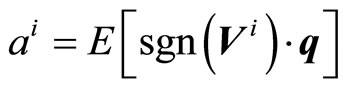 (10)
(10)
In similar manner, the value of  can be found by minimizing the MSD between the modulated codeword and the vector representing the vertical sum of
  . Suppose that
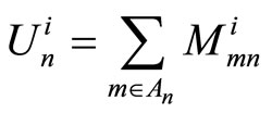 (11)
(11)
and let the vector  , then
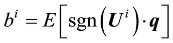 (12)
(12)
It is worth mentioning that both Equations (10) and (12) need to be computed to the transmitted codeword q and this is not available at the receiver in real-world systems. It is suggested to solve this problem in three different ways. First, it is possible to compute the values of  and
and  offline for different channel characteristics and store their values in memory to be used latter by the decoder online. This will reduce the proposed modification to simple multipliers. Second, pilots and headers are known signals to the decoder, so they offer online estimation for the correction factors. Third, from the simulation of different systems, it is observed that the values of
  and
and  have nearly stationary values for certain number of iterations, code parameters and channel characteristics. Thereby sending few known codewords to the receiver at the start of or in between transmission is sufficient to compute the correction factors with accepted accuracy.
Actually, for certain code H and channel characteristics (s) (e.g.,  ), the correction factors are function of the iteration’s number (i) and the number of simulated frames (t), (i.e.,
  and
and  ). The average values of
  over all simulated codewords is given by
 (13)
(13)
Further, if the average is done over all iterations, we get
 (14)
(14)
And finally, the averaging over all simulated values of  produces a constant
 (15)
(15)
Different simulation tests are carried out to demonstrate the effect of averaging presented in Equations (13)- (15) on the error performance of LDPC.
4. Implementation by Software-Defined Radio
To be close from the implementation issues of the realworld wireless communications, semi-practical tests to some of the simulated systems are experienced using the MATLAB data acquisition toolbox and PC sound card. Real-world passband signals for some of the modified and unmodified coded systems are transmitted and received via room-to-room audio sender operating in the 2.4 GHz industrial, scientific and medical (ISM) radio band. The acquired signal from the PC sound card can be directed to the RAM and/or the hard disk to be processed later by the SDR receiver. The SDR receiver takes consider of all the required DSP algorithms like modulation/ demodulation, pulse shaping filtering, synchronization and signal to noise power ratio (SNR) estimation in MATLAB code.
Figure 1 depicts simple Graphical User Interface (GUI) panel that used as SDR receiver.
The panel offers different options that can be changed to suit the desired test like codeword length (N), coding rate (R), maximum number of iterations (imax), baud rate and oversampling value. It is also possible to change the order and roll-off factor of the square root raised cosine filter which is used in pulse shaping process for the transmitted and received signals.
Figure 2 shows the block diagram of the proposed SDR system. While, Figure 3 depicts a picture for the set of SDR test system.
In asynchronous data transmission, the frame and bit
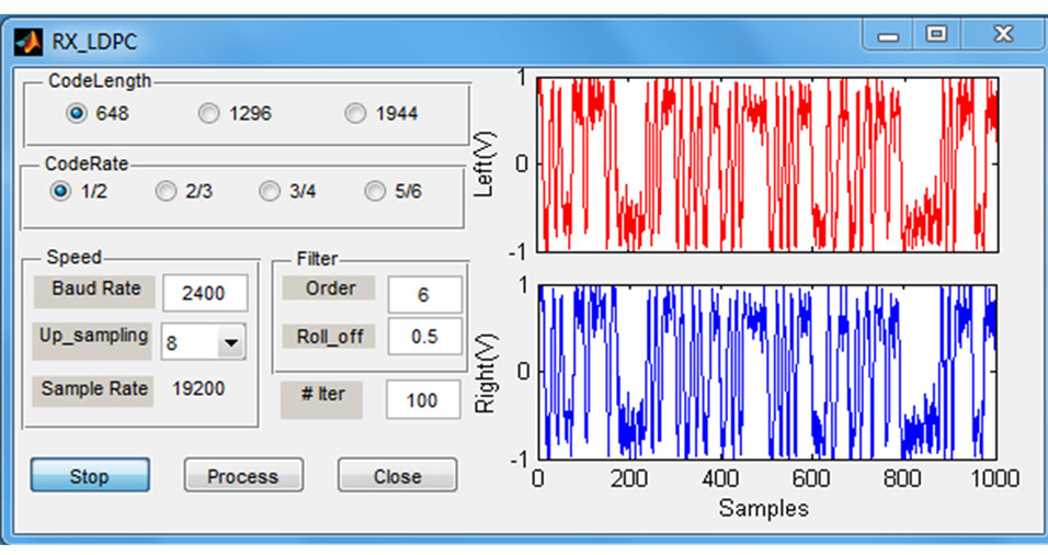
Figure 1. GUI panel used for SDR receiver.
synchronization are considered as a challenging problem. In this study, a simple frame construction is considered to cope with this problem as shown in Figure 4. In the front of any transmitted frame a header is generated by one or more Barker code(s) of thirteen bits in length. The length of the header determines the capability of the receiver to mark the starting point of the received frame and reduces the probability of miss detection. However, the quality of the channel is the main factor in determining the header length.
Intuitively, the data followed the header is random for the receiver which leads to a mismatch between the actual and reference header at the receiver due to filtering process. This is manifested especially at the junction between the header and data fields. Since the header signal is utilized to estimate the SNR, this undesirable distortion will reduce the accuracy of estimation. Therefore, three bits (e.g., 101) are appended by the header bits. The padded bits should be omitted during the SNR estimation to get rid of this distortion. Figure 5 illustrates a section from the transmitted frame at the junction between header and data, received noisy signal, and the output of
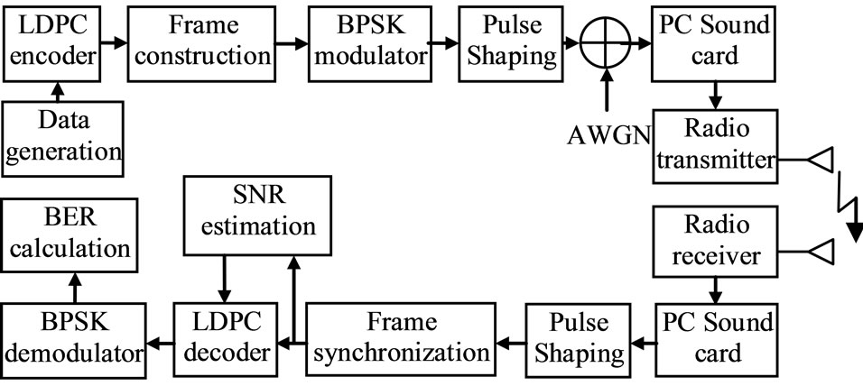
Figure 2. Block diagram of the proposed SDR system.
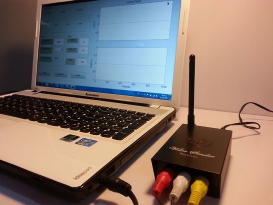
Figure 3. The experimental set of the SDR system.
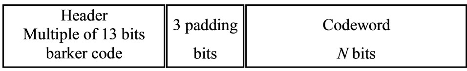
Figure 4. Frame construction.
square raised cosine filter. The estimated  at the receiver is around 15 dB for this case.
The SNR estimation technique presented here originated from a method for measuring channel distortion errors in wideband telemetry systems [15], in which the noise in a signal at a point in a system is defined as the mean-square error (MSE) between the actual signal and a desired signal at that point. The estimated SNR is given by
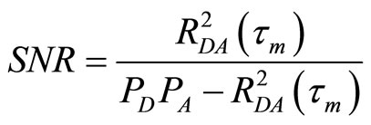 (16)
(16)
where  and
and  represent the average powers in the reference (desired) header and the actual (received) header, respectively. The maximum correlation
 between the actual and the desired header signals indicates the system time delay
 .
.
Figure 6 demonstrates the correlation between the reference and actual headers. The maximum correlation  marks the beginning of the received frame. It is worth mentioning that the abscissa of the BER performance graphs for the practical tests presented in section 5.2 is the average of the estimated SNR over all transmitted frames.
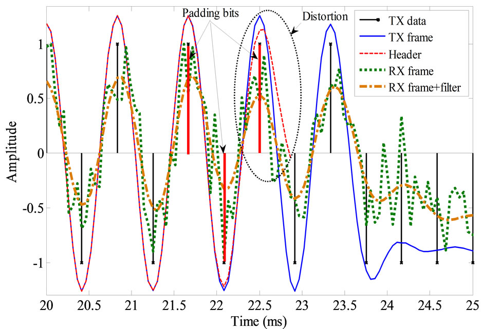
Figure 5. Transmitted data, transmitted pulse shaped, received noisy and filtered signals (part of).
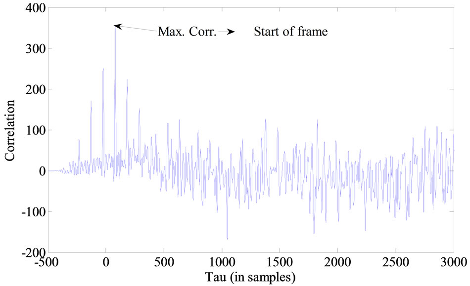
Figure 6. Correlation between desired and actual headers.
5. Simulation and Practical Results
5.1. Simulation Results
Simulations are carried out over the AWGN channel with BPSK modulation for the proposed 1-D and 2-D corrected MS decoding for LDPC code which is adopted by the standard IEEE 802.11n [2]. Figure 7 presents the BER performance of regular (1944, 1296) rate 2/3 LDPC with the decoding algorithms; SP, original MS, 1-D MS-( ), 1-D MS-(
 ) and 2-D MS-(
 ). The systems in Figure 7 (excluding 1-D MS-(
 )) are retested using the regular (648, 324) rate 1/2 LDPC and depicted in Figure 8. It is obvious that the performance gap between the proposed 2-D MS-(
 ) and the SP decoders is only of 0.1 dB and 0.04 dB at BER = 10−4 for the (1944, 1296) and (648, 324) codes, respectively.
Table 1 illustrates the values of the correction factors as, bs, a, b and the mean value of a and b, i.e.,  , for the (1944, 1296) rate 2/3 LDPC code.
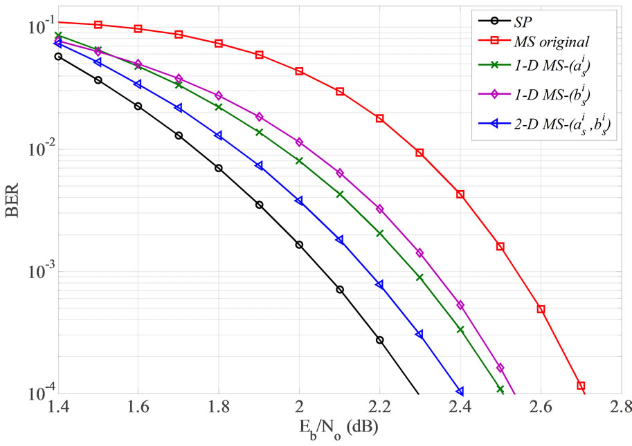
Figure 7. BER performance of SP, original MS, 1-D MS-  , 1-D MS-
 and 2-D MS-
 decoding algorithms for regular (1944, 1296) LDPC,
  .
.
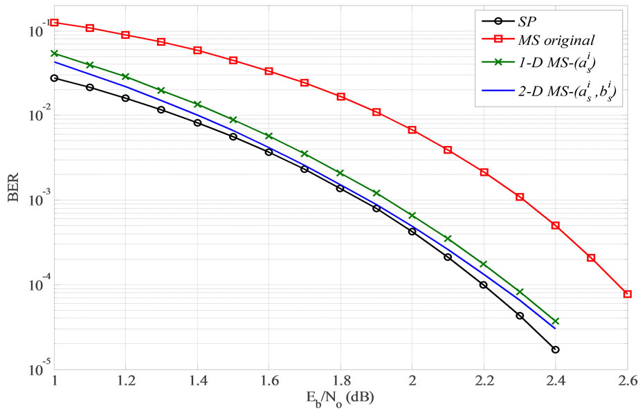
Figure 8. BER performance of SP, original MS, 2-D MS-  and 1-D MS-
 decoding algorithms for regular (648, 324) LDPC,
  .
.
It is interested to note that the values of as and as are very close to each other, so it is possible to use the same correction factor at the bit and check node for more reduction in complexity.
Figure 9 demonstrates the effect of applying the average of correction factors over all iterations and further over the whole tested range of  . It is clear that the averaging of the correction factors over all iterations (as, bs) results a deterioration in error performance, but only about 0.02 dB.
Applying a and b instead of as, and bs in MS decoding gives a slight improvement especially at high SNR. This interested result urged on testing the proposed scheme by applying a single correction factor  = 0.889 at the bit and check nodes for the whole range of SNR and along all decoding iterations. The 2-D MS-
 decoding scheme shows a reduction in performance in comparison with other schemes at low
  . After
  dB the BER performance of this scheme outperforms the 2-D MS-(as, bs) and 2-D MS-(a, b) systems and becomes even better than the 2-D MS-
 scheme after
  dB.
dB.
Figure 10 presents the probability of failure for the (1944, 1296) LDPC, for SP, original MS, and 2-D MS-  decoding algorithms. Probability of failure can be
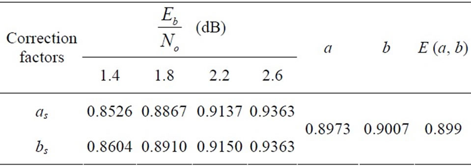
Table 1. Correction factors  , their average values (a, b) and the average of a and b of regular (1944, 1296) LDPC.
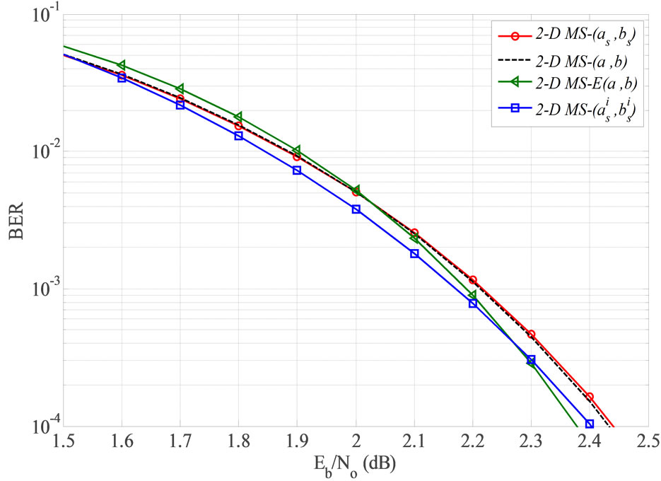
Figure 9. BER performance of 2-D MS- , 2-D MS-
  , 2-D MS-(a, b) and 2-D MS-
 decoding algorithms for regular (1944, 1296) LDPC,
  .
.
defined as the probability of the decoder to reach the maximum number of iterations  without satisfying the parity check equations, i.e.,
  . Figure 11 shows the average number of iteration for each simulated system in Figure 10. It is clear from Figures 10 and 11 that the modified MS decoder demonstrates a comparable performance to the optimum SP decoder.
Figure 12 presents the variation of  and
and  over 100 iterations with different values of
  . Figure 13 demonstrates the values of
  over the simulation of 50 and 500 frames. It is clear that the two curves are very close to each other which mean that it is possible to estimate the correction factors online with few known received frames without losing a lot of time in this process.
5.2. Practical Results
Experiments of wireless indoor transmission (utilizing the SDR approach explained in Section 4) are carried out to prove the effectiveness of the proposed systems. The tests are running over approximately the same environ-
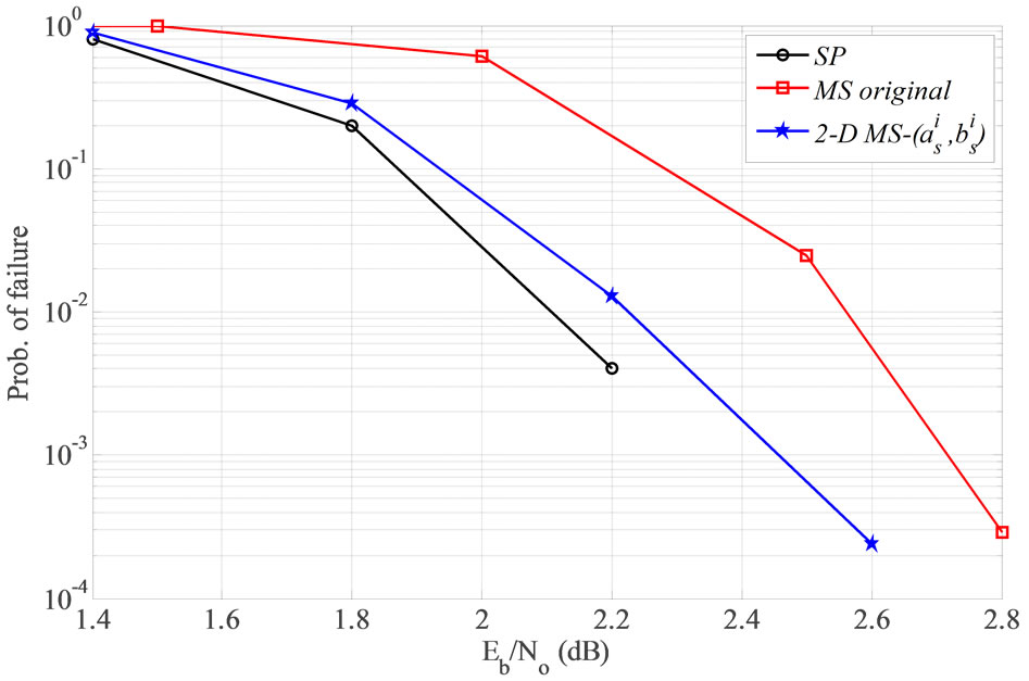
Figure 10. Probability of failure of SP, original MS and 2-D MS- algorithms for regular (1944, 1296), 2/3 rate LDPC.
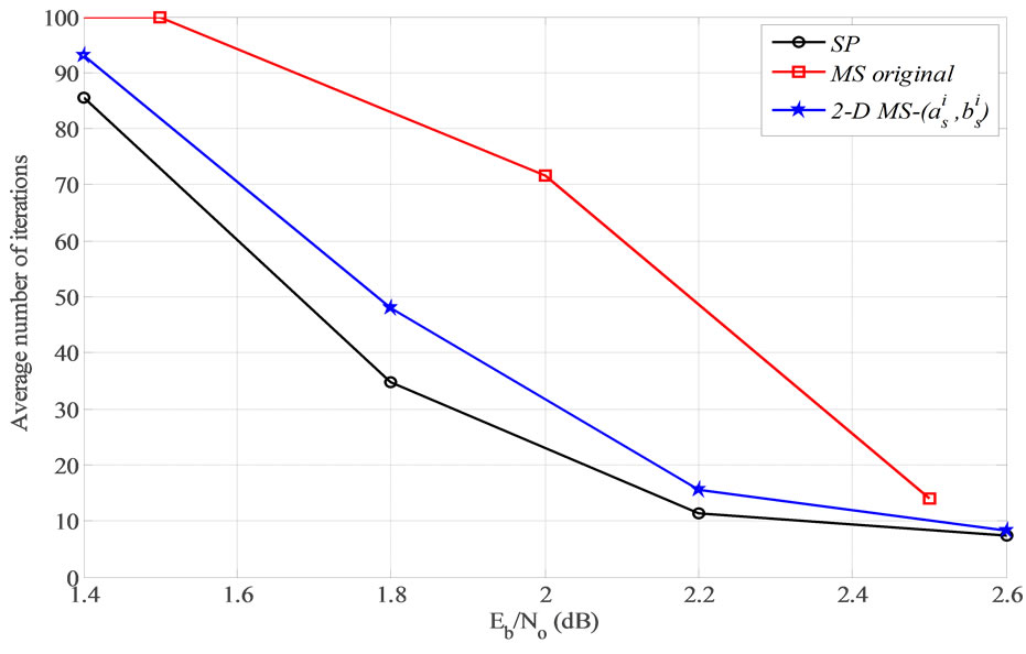
Figure 11. Average number of iteration of SP, original MS and 2-D MS- algorithms for regular (1944, 1296), 2/3 rate LDPC.
ments. The transmitter and the receiver are fixed inside a 4 m ´ 4 m room during the experiments. The data is transmitted with a bit rate of 2400 bit/sec using BPSK modulation. The filter order and roll-off factor at both transmitter and receiver are adjusted to 6 and 0.5 respectively.
Figure 14 presents the resulted BER performance of original MS, 2-D MS- , and 2-D MS-E(a, b) decoding algorithms of the regular (1944, 1296) LDPC code. It is noted that the BER performance of the proposed 2-D MS-
 , decoder outperform the original MS by about 1.1 dB measured at BER = 10−3. Reducing the complexity by using one correction factor
  for both bit and check messages results in reduction of performance by about 0.12 dB in compare with the 2-D MS-
 decoding. Table 2 illustrates the correction factors (as, bs), their average values (a, b) and the mean value of a and b, E(a, b) that acquired from the practical test of the regular (1944, 1296) LDPC code.
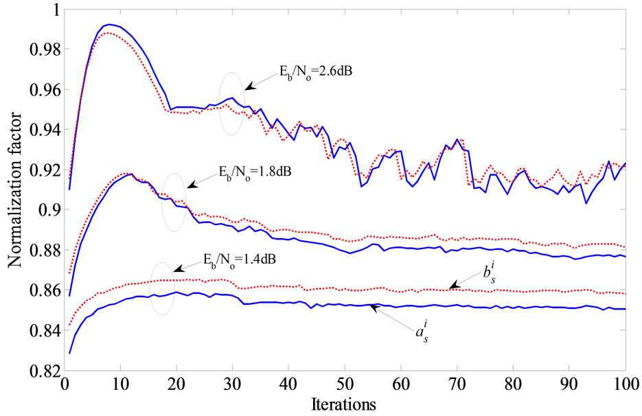
Figure 12. The correction factors  and
and  over 100 iterations with different
  .
.
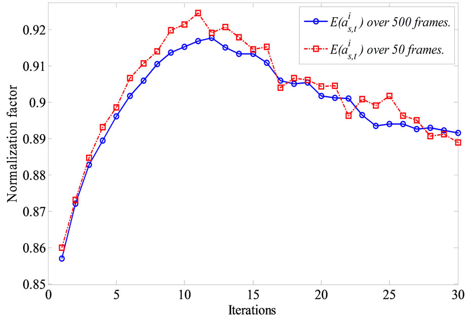
Figure 13. The average of correction factor  over t = 50 and 500 transmitted frames of regular (1944, 1296), 2/3 LDPC at
  .
.
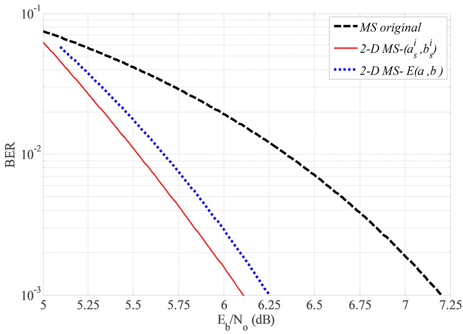
Figure 14. BER performance of original MS, 2-D MS-  , and 2-D MS-E (a, b) decoding algorithms of the regular (1944, 1296) LDPC code.
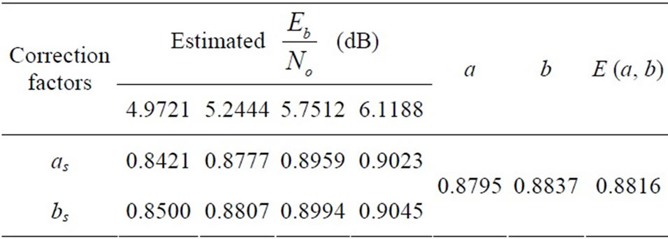
Table 2. Correction factors (as, bs) and their average values (a, b) for practical test of the regular (1944, 1296) LDPC code.
6. Conclusion
In this paper, a 2-D corrected MS decoding has been presented to improve the performance of standard MS decoding. Simulation and practical tests show that 2-D corrected MS provides a good performance versus complexity tradeoff for decoding regular LDPC codes. In comparison with the standard SP, the proposed method requires considerably less complexity while introducing small performance degradation, especially if a single correction factor for both check and bit nodes is considered. Further analysis and hardware can be done for irregular LDPC codes.
REFERENCES
- R. G. Gallager, “Low-Density Parity Check Codes,” IRE Transactions on Information Theory, Vol. 8, No. 1, 1962, pp. 21-28.http://dx.doi.org/10.1109/TIT.1962.1057683
- IEEE 802.11n, “Wireless LAN Medium Access Control and Physical Layer Specifications: Enhancement for Higher Throughput,” IEEE P802.11n/D1.0, 2006.
- IEEE 802.16e, “Air Interface for Fixed and Mobile Broadband Wireless Access Systems,” IEEE P802.16e/D12 Draft, 2005.
- European Telecommunications Standards Institude (ETSI), “Digital Video Broadcasting (DVB) Second Generation Framing Structure for Broadband Satellite Applications,” EN 302 307 v1.1.1, 2005.
- N. Wiberg, “Codes and Decoding on General Graphs,” Ph. D. Thesis, Linkoping University, Linkoping, 1996.
- M. P. C. Fossorier, M. Mihaljevic and H. Imai, “Reduced Complexity Iterative Decoding of Low-Density Parity Check Codes Based on Belief Propagation,” IEEE Transactions on Communications, Vol. 47, No. 5, 1999, pp. 673-680.
- J. Chen and M. P. Fossorier, “Near Optimum Universal Belief Propagation Based Decoding of Low Density Parity Check Codes,” IEEE Transactions on Communications, Vol. 50, No. 3, 2002, pp. 406-414. http://dx.doi.org/10.1109/26.990903
- J. Zhang, M. Fossorier, D. Gu and J. Zhang, “Two-Dimensional Correction for Min-Sum Decoding of Irregular LDPC Codes,” IEEE Communications Letters, Vol. 10, No. 3, 2006, pp. 180-182.
- V. Savin, “Self-Corrected Min-Sum Decoding of LDPC Codes,” ISIT 2008. IEEE International Symposium on information Theory, 2008. ISIT 2008, Toronto, 6-11 July 2008, pp. 146-150. http://dx.doi.org/10.1109/ISIT.2008.4594965
- H. Wei, J. G. Huang and F. F. Wu, “A Modified MinSum Algorithm for Low-Density Parity-Check Codes,” 2010 IEEE International Conference on Wireless Communications, Networking and Information Security (WCNIS), Beijing, 25-27 June 2010, pp. 449-451.
- X. F. Wu, Y. Song, L. Cui, M. Jiang and Ch. Zhao, “Adaptive-Normalized Min-Sum Algorithm,” 2010 2nd International Conference on Future Computer and Communication (ICFCC), Wuhan, 21-24 May 2010, pp.V2-661- V2-663.
- A. A. Hamad, “Performance Enhancement of SOVA Based Decoder in SCCC and PCCC Schemes,” Scientific Research Magazine, Wireless Engineering and Technology, Vol. 4, No. 1, 2013, pp. 40-45. http://dx.doi.org/10.4236/wet.2013.41006
- T. J. Richardson and R. L. Urbanke, “Efficient Encoding of Low-Density Parity-Check Codes,” IEEE Transactions on Information Theory, Vol. 47, No. 2, 2001, Article ID: 638456.
- D. J. C. MacKay, “Good Error-Correcting Codes Based on Very Sparse Matrices,” IEEE Transactions on Information Theory, Vol. 45, No. 2, 1999, pp. 399-431. http://dx.doi.org/10.1109/18.748992
- T. H. Shepertycki, “Telemetry Error Measurements Using Pseudo-Random Signals,” IEEE Transactions on Space Electronics and Telemetry, Vol. 10, No. 3, 1964, pp. 111- 115. http://dx.doi.org/10.1109/TSET.1964.4335603