Smart Grid and Renewable Energy
Vol.06 No.04(2015), Article ID:56069,17 pages
10.4236/sgre.2015.64009
Comparison and Simulation of Building Thermal Models for Effective Energy Management
Fatima Amara1, Kodjo Agbossou1, Alben Cardenas1, Yves Dubé2, Sousso Kelouwani2
1Department of Electrical and Computer Engineering, University of Quebec at Trois-Rivieres, Trois-Rivieres, Canada
2Department of Mechanical Engineering, University of Quebec at Trois-Rivieres, Trois-Rivieres, Canada
Email: fatima.amara@uqtr.ca
Copyright © 2015 by authors and Scientific Research Publishing Inc.
This work is licensed under the Creative Commons Attribution International License (CC BY).
http://creativecommons.org/licenses/by/4.0/


Received 17 February 2015; accepted 29 April 2015; published 30 April 2015
ABSTRACT
Energy consumption reduction efforts in the residential buildings sector represent socio-eco- nomical, technological and environmental preoccupations which justify advanced scientific research. These lead to use inverse models to describe thermal behavior and to evaluate the energy consumption of buildings. Their principal goal is to provide supporting evidence of enhanced energy performances and predictions. More specifically, research questions are related to building thermal modeling which is the most appropriate in a smart grid context. In this context, the models are reviewed according to three categories. The first category is based on physical and basic principle modeling (white-box). The second offers a much simpler structure which is the statistical models (black-box). The black-box is used for prediction of energy consumption and heating/ cooling demands. Finally, the third category is a hybrid method (grey-box), which uses both physical and statistical modeling techniques. In this paper, we propose a detailed review and simulation of the main thermal building models. Our comparison and simulation results demonstrate that the grey-box is the most effective model for management of buildings energy consumption.
Keywords:
Building Control, Inverse Modeling, Building Prediction Model, Simplified Building Models, Parameters Estimation

1. Introduction
Energy policies in the Nordic countries, such as Canada, stipulate that 50% of the energy consumed by 2025 should come from renewable and CO2-free energy sources [1] . By 2050 the aim is to be independent of fossil fuels. This transition of the energy systems towards renewable sources is needed to reduce CO2 emissions and consequently reduce the speed of global warming. Moreover, this transition is a contributing factor to protect Nordic economies from the consequences of sharply rising prices of fossil fuels which can be attributed to an increasing demand and depletion of these non-renewable resources [1] . Transition to renewable energy sources are not only preoccupations for Nordic countries. Indeed, all industrialized countries [1] , including China and the United States, are concerned about these. For example, in the United States alone the total energy consumption increased from 78.3 quads in 1980 to over 100 quads in 2008. Of this amount, buildings are responsible for more consumption than transportation or industry sectors, accounting for nearly 40% [2] of the total non-re- newable energy consumption in the U.S. The building sector is also responsible for almost 40% of greenhouse gas emissions and 70% of electricity use in this particular country.
Buildings energy consumption is imputable mainly to heating/cooling, lighting, and electrical appliances. In Nordic countries, heat pumps, water based heating systems, water heater and electric baseboard heaters are of the main loads for heating [1] . As a result of the efforts towards the renewable energy transition, the U.S. and other countries are committed to invest into smart grid technologies to minimize the overall energy cost of electricity. Smart grid can reduce energy consumption, increase the efficiency of the electricity network, and manage electricity generation from renewable technologies. In fact, as illustrated in Figure 1, China is in the lead position for renewable energy investments, with about $7.3 billion stimulus spending in 2010. More specifically, China developed a large, long-term stimulus plan in water systems, rural infrastructures and power grids, including a substantial investment in smart grid technologies [2] . Several Nordic countries, such as Canada, while having different priorities for defining their clean energy strategies, are having an important role in the implementation of smart grid technologies [3] . In Canada, the various government electricity ventures are to invest $11 billion in total towards innovative infrastructure replacement for the next 20 years. For this effort, there are also The Canadian Smart Microgrid Research Network and the Smart Grid Standards Task Force [2] , which is contributing to providing leadership through their participation in new initiatives [2] . Canada has a leadership role to play in energy efficient building in North American, as well as around the world, for smart grid implementation. In fact, this leadership is already evidenced by the innovative culture and the technical expertise available in many areas across the country [2] . However, the ways to make use of smart grid technologies to improve building energy efficiency is still an open issue. For example, energy efficiency of buildings, in thermal and electric aspects, can be leveraged to improve the smart grid efficiency and reliability.
The study of buildings and grid interactions in the new smart grid scenario is then necessary. This study starts with a thermal and electric modeling of buildings. Its goal is to provide a review of the subject of energy effi-

Figure 1. Ranking of top 10 countries receiving smart grid federal stimulus investments in 2010. (From Zpryme Research and Consulting, 2010) [3] .
ciency and buildings modeling in the context of smart grid. In Section 1, the state of the art is presented. Section 2 gives a review of the most important approaches used in thermal modeling of buildings. Section 3 provides a condensed comparison of the white, black and grey-boxes modeling approaches. Section 4 is devoted to summarizing the importance of the thermal modeling in the implementation of prediction techniques of energy consumption taking into account weather predictions to increase energy efficiency of buildings. Section 5 gives an example of simulation of black and grey-boxes approaches. Finally, Section 6 presents concluding remarks and identifies a number of research and policy needs.
2. Approaches of Thermal Modeling of Buildings
In recent years, a variety of works in the area of thermal modeling of buildings has been done and can be found in the literature [4] -[6] . This review focuses on the model structure, more specifically the analysis of imposed information flow path between the thermal inputs and the thermal outputs of buildings. These thermal models are used to identify energy savings or efficiency of buildings [7] .
As such, many models have been made to improve the energy efficiency in buildings. Some aim for residential buildings, some for commercial buildings, and some for both [8] . Not all of these models are cost-effective for all cases. Indeed, it is important to analyze the different modeling approaches to ensure increased efficiency of buildings’ system, because space and water heating along with air conditioning are the main residential loads [9] . Those three are the major energy consumption devices [8] . Consistently to these main residential loads, a variety of thermal models have been proposed [10] -[12] .
Generally, the proposed models are characterized by two thermal behaviors. The first one is a static behavior, while the second one is dynamic. The static behavior is applied to simplify the thermal model and to overcome the limitations of computing resources. The dynamic behavior is interested in understanding the phenomenon of thermal exchange for simulation purposes.
2.1. Modeling Approaches
The static behavior approach is used for steady state conditions of buildings, when all the internal and external inputs are controllable. The dynamic behavior approach is related to the transition of internal and external inputs and outputs of the building system [13] . Thus, a substantial number of models of the static and dynamic approaches have been used in the presentation of the thermal behavior of buildings. It was proposed to classify the sets of these models into three categories, the white, the black and the grey boxes models as illustrated in Figure 2. Depending on the static and dynamic approaches, some of the models have been very successful in describing the thermal behavior of large residential buildings. Others have been used to estimate the thermal-energy demands or in the prediction of heat consumption and reducing energy consumption. However, in the context of energy efficiency of buildings and smart grid implementation, our study focuses only on dynamic models. Therefore, it is using the dynamic behavior approach only that the black, white and grey boxes models are described in the present study.
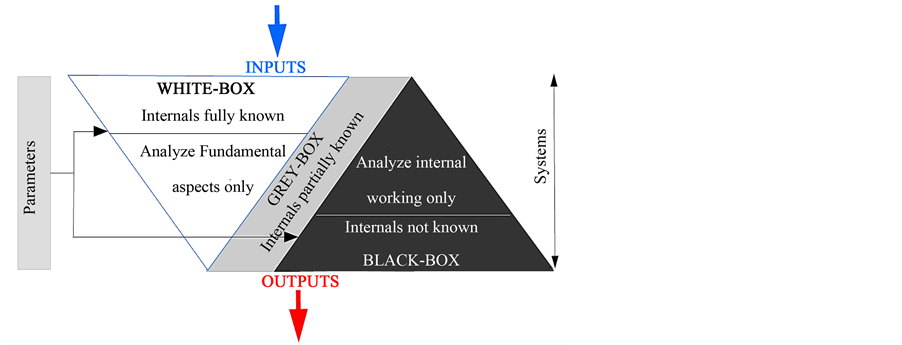
Figure 2. Black box, white box and grey box behavior [14] [15] .
In fact, considerable attention has been placed on the black, white and grey models in dynamic approach which include the thermal networks, modal analysis, differential equations, autoregressive moving average model (ARMA), Fourier series [11] -[13] [16] [17] , and the transfer functions [18] . While other studies use these models for the prediction of heat consumption, few comparisons exist for their robustness to new control situations [9] [19] -[21] , or their applications to smart grid building types [12] . Comparisons between approaches are important since, at some stages in the future of smart grid and buildings efficiency, these may become unattractive for energy management of peak demand at the residential level. This will likely be the case for scheduled of household appliances or other situations for which power consumption levels within predefined operation duration are the main decision variables [22] . Also, high occupancy levels and great number of technical devices, such as computers and printers, cause high internal loads [13] [23] . Therefore, for a successful modeling of a building, it is critical to consider how much we know about these variables.
2.2. Discussion on the Physical and Statistical Models
In practice, residential buildings are more variable in occupancy and internal heat gains due to appliances and all other electrical driven equipment. Appliances driven loads and gains are divided into two classes. The first one corresponds to the responsive loads which indicate that the customer is able to modify the behavior of the appliance due to a price signal. This class includes lights, plug loads, clothes washers, clothes dryers, dishwashers, cooking ranges, and microwaves. The second class is the unresponsive loads appliances, which indicate that the customer is typically not able to modify the behavior without investment in additional technologies. This class includes refrigerator and freezer loads [24] . In regards to electric heaters, with a responsive thermostat which controls the output of the heater effectively and maintains a more consistent room temperature, the electric heaters models without a thermostat require closer monitoring by the customer, and therefore are associated with unresponsive loads [8] .
Considering thermal phenomena, heat transmission, heat storage, fluid flow and heat flux represent the fundamental thermal properties of building elements. These phenomena are highly time-sensitive [25] . Consequently, the question of which model structure is required for thermal description of residential buildings with the presence of all phenomena cited above arises. Also, the question about the deterministic and stochastic parameters also arises to perform the system identification. Finally, the last question is about which models should be used in an energy consumption prediction framework. As a rule of thumb, if enough building knowledge is available to describe the set of heat transmission, heat storage and heat flux, and the corresponding parameters with physical significance, then these can be described by fundamental physical principles. In this case, the answer to the question regarding model structure and the parameters are answered by the “white-box” models, which will best describe all the phenomena and predict heat consumption efficiently [26] . Indeed, the white-box models can be constructed from the prior information without the need of any observation. However, if the phenomena of residential building are too complex to be described by physical fundamental principles, but can be observed or measured, then the “black-box” models are appropriate. These models are characterized by an input-output behavior without any detailed information about the structure. Finally, if the set of phenomena of residential building are both directly observable and have physical meaning, the “grey-box” can be applied to estimate the thermal-energy demands and predict the heat consumption.
3. Comparative Study of White, Black and Grey Box Modeling Approaches
3.1. White-Box Model
In the case of physical model with parameters of physical significance, we speak of a white-box (physical and basic principle modeling) approach, which require a significant amount of building knowledge [14] [27] . White-box models can be defined by the equations in Table 1. These models they are based on:
・ Static and dynamic models;
・ Linear, nonlinear models;
・ Differentiable, continuous, non-continuous models.
In static models the output of system does not depend on the time. While in dynamic models, the output is time varying due to the dynamic heat balance time evolution. These dynamic white-box models are typically represented by differential equations. However, their mathematical representation also depends on the relation

Table 1. Examples of different equation types of white-box model [28] .
between the parameters. These relations can be ordinary, partial, linear and non-linear differential equation, we propose to sum up these mathematical representations in Table 1.
The complexity of white-box modeling depends mainly on the chosen precision`s levels of the known phenomena associated with the building system to be modeled [28] . White-box models can be usually even the classical error calculation methods which are applied to determine predictive accuracy of the models. That is, even if the parameters of white-box models have physical significance (e.g. thermal conductivities of certain materials), and fundamental physical principles are used, there are always errors associated with random variables that are not represented in the known parameters (e.g. window openings and air exchange rates in natural ventilation) [28] . When calibrating white-box models, it is useful to make sense to adapt the less precisely known parameters (i.e. heat transmission, heat storage and heat flux), where usually plausible constraints on these parameters are determined.
If the model cannot be calibrated, this suggests that the model structure has to be questioned. In the literature, it is suggested that a too high number of parameters can be a significant source of error [29] [30] .
Black-box models are empirical models (statistical) without physically significant parameters. That is, contrary to the white-box, when little is known about the inner workings of the building system. This means that black-box models are derived the inputs-outputs thermal behavior. This case is black-box approach [14] [31] . Their internal structure of black-box model does not reflect the structure of the building system phenomena. Black-box models focus on finding the relationships between input and output variables, independently of the building system phenomena or random variables, which are affecting the predictive efficiency of the white-box approach.
3.2. Black-Box Model
In the black-box, the parameters are generally adjusted automatically [32] . This automatic adjustment of calibration of black-box parameters provides the greatest benefit over white-box models. However, a disadvantage is their implicit relationship with physical fundamental principles. Indeed, black-box model identification is found to be inconsistent with physical reality when applied under hard conditions (little building system data) [33] . Therefore, black-box models are mainly used for error detection, but not for the optimization. Their advantage is the rapid and automated identification of outputs of thermal energy building consumption. With respect to the model internal structure of black-box models it can be static and dynamic, linear and nonlinear models, just as the white-box models. The structure depends on the relationships between the input and output data. Depending on these relationships, various black-box methods for estimating the parameters (calibration) are available. Table 2 gives an overview of the different approaches.
In thermal modeling of buildings, it is reasonable to combine the relative strengths of black-box coming from the statistical with the white-box strengths based on physical interpretation [31] [33] in order to obtain an a hybrid model. In that sense, the standard “grey-box” approach is based on both, a statistical method and physical properties that meets the physical fundamental principles.
3.3. Grey-Box Model
Grey-box models are therefore mixed or transitional forms of white-box and black-box models. There are in the literature several definitions; the following are the most frequently encountered:
・ Definition 1 (type of parameters)
Grey-box parameters are both empirical and have a physical significance [29] .
・ Definition 2 (determination of the parameters)
Grey-box models are characterized by the fact that all their parameters or a part of them are determined on the basis of measured data of real system [6] [30] .
Definition 2 does not define any kind of model, but rather the manner of determining the parameters of a model. It should be mentioned that in the literature, often the term Hybrid model emerges. Independently of the terms or definition used, grey or hybrid models, this approach cannot inform on the particular composition of various phenomena parameters from the white or black models. That is, we just know that there is a mixture of both models without knowing which one dominates in the combination of white-box and black-box models [6] [30] ,. This combination is automatically done, depending on the problem and the choice of basic functions for example (linear, polynomial or harmonic functions) adapted to the simulation results. Grey box models can be developed for the individual components or for a larger complex system. Table 3 provides an overview of the most important properties regarding the three different modeling approaches (white-box, grey-box and black- box) discussed above including calibration, and application.
Table 2. Overview on black-box models [27] .
Table 3. Summary of the advantages and disadvantages of different types of models [28] [31] .
As illustrated in Table 3, white-box models have good analysis skills, but, they require an increased effort in the calibration of parameters. Also, white-box models with a simple structure model have possibly lower prediction accuracy. White box models are initially very useful for the understanding of physical fundamental system. On the other hand, black-box models are well suited to existing patterns (e.g. to identify quickly the consumption profiles for building) [28] .
Grey-box modeling can be useful to understand the parameters which can lead to significant errors in predicting units’ consumption [34] . They are particularly useful in the following cases. First, when there is a lack of detailed information building phenomena and the thermal mass, e.g., walls, floor, ceiling, room air, etc. This information affects the thermal dynamics of the building [22] . Secondly, when there is uncertainty of the end usage and behavior of the occupants. Finally, when there is limited capacity of the means of calculation and experimental building [24] . For all of these cases, grey-box modeling can increase the optimality of the energy management of other loads, such as HVAC and water heating. In fact, such modeling can smooth the load factor during peak hours, enhance reliability and efficiency in power networks and reduce operational costs [35] .
The next section focuses on the link between the grey-box models and the model predictive control of building systems. We will briefly describe the need of a structural model based on semi-physical laws and the basic ideas lying behind the prediction method in building to improve performance buildings and reduce the energy consumption of heating and cooling systems [36] .
4. Finding a Thermal Model for Energy Prediction
The key to the sustainability of the energy efficiency of buildings [37] is the analogy between the thermal models and the prediction methods of energy consumption. This analogy is the most important goals of smart grid technologies [38] . However, it is important to analyze the relation between the whole of phenomena of heat transmission, heat storage, and the variation of the demand of cooling and heating of residential building to predict the energy consumption. Also, black-box, white-box or grey-box thermal models are trained using these relations [39] . In smart grid context, the application of accurate and complete thermal model, conduct to increasing the efficiency of HVAC systems by natural ventilation. Indeed, reducing the heat consumption returns to the ability of the model to describe the different internal and external phenomena of building. For this point, it must have a good thermal behavior representation of building through the fundamental physical concepts by the statistical models or rather a mixture of the both.
There are several completely different approaches to system identification (see e.g. [40] -[42] ). Some of them exploit both the principle physical and statistical data of building system. For example, grey-box [43] [44] (some prior information such as system structure is known in advance) or black-box identification [45] . Dynamics behavior of building is argued that the residence includes three intrinsic factors on its structure. First, when the group includes the composition, the surface to be heated, etc. Secondly, when the group includes the phenomenon related to the weather/climate data, such as solar radiation I (W/m²), wind speed (m/s) and the outdoor temperature out (˚C) [23] . Finally, when the group represents the interactions factors with the building, the occupant profile, the power Q (W) demanded by HVAC, and water heating systems [13] .
We addressed the question: how to describe the response of the indoor temperature in the presence of the different internal phenomena such as the heat transmission, heat storage, and the external phenomena of consumption able to improve the energy performance of a building, in order solar gains, wind speed and outdoor temperature? [27] . In parallel, define the predictive method of energy to improve the energy performance of a building, conserve energy, reduce environmental impact, control the use of energy over time, move energy consumption to off-peak periods [46] . One of the basic tenets to minimize energy consumption is the understanding of buildings thermal phenomena is the usage patterns (profiles), and local environment. This information is frequently not known a priori [47] .
Generally, the need of a complete and detailed heat balance equation should incorporate the effects of different sources: the weather (temperature, humidity, solar radiation and wind speed) [48] , and the calculation of the heat flow within a building such as internal gains from waste heat generated by loads. These sources and sinks of heat constitute the total heat energy exchange in the house as illustrated in Figure 3. Although, the flow of heat is divided between the air and the mass of the house (i.e., walls and furniture), a portion of the incident solar energy through a window will heat the interior air of the house, while the remaining incident energy will be absorbed by the walls, floors, and furniture.
As it was discussed above, it is easier in this case to describe these phenomena by grey-box modeling approach [4] . This approach is based on semi-physical laws analog circuit model such as the equivalent electric circuit (RC). The (RC) model can be presented as form as mathematical expressions (algebraic, differential equations) in which can distinguish between deterministic and stochastic parameters. These parameters cannot be directly observable (indirect measurement) and estimated [26] [50] depending on the a-priori and a posterior information of building system.
Describing the transit thermal behavior by grey-box and capture the evolution of the indoor temperature of building is presented in section V. Thus, it is convenient to introduce the concept of thermal capacity of building denoted by , in the electric circuit analog model (RC) that is used to describe heat flow and heat transfer phenomena as illustrated in Figure 4. Where,
  equal to the air mass
  in the room times the specific heat capacity of air
  which change with timeas shown in the following Equations (1) and (2):

Figure 3. Simplified diagram of sources and sinks of heat in a house [49] .

Figure 4. The RC model of residences heating/cooling system [52] [53] .
 (1)
(1)
With
 (2)
(2)
And  is the density of air at the room temperature. V is the volume of the room [2] [50] . The heat transfer properties in this case are represented by equivalent electrical components with associated parameters for modeling the thermostatically controlled HVAC system. The thermal model building proposed in [51] assumes that only envelope characteristics, solar gain through windows and internal gain contribute to the heating, ventilation, and air conditioning (HVAC) load.:
where:
 : air heat capacity (Btu/˚F or joules/˚C);
 : mass (of the building and its content) heat capacity (Btu/˚F or joules/˚C);
 : the gain/heat loss coefficient (Btu/˚F.hr or W/˚C) to the ambient;
 : the gain/heat loss coefficient (Btu/˚F.hr or W/˚C) between air and mass;
 : outdoor temperature (˚F or ˚C);
 : air temperature inside the house (˚F or ˚C);
 : mass temperature inside the house (˚F or ˚C);
 : heat added to the indoor air;
 : heat added to the building mass.
Heat balance equation solved of the (RC) model for the air temperature node  is given by the Equation (3) [53]
 (3)
(3)
And the heat balance for the mass temperature node  is given by the Equation (4) [53]
 (4)
(4)
Depending to the application, to the complexity of modeling and to the set of phenomena of residential building to described. The (RC) model parameters can be used to represent all homes in the population for simplicity. Or if there is a need, multiple RC models with different thermal parameters can be used. In addition to changing input parameters while simulating a population of homes, the (RC) model can also be changed to accurately represent a given building stock [51] .
Hence, the prediction models are needed to enable optimal control of buildings phenomena [54] and also, to predict dynamic cooling and heating requirements for the building. In particular the thermostat controllable loads such as electric water heater, heat-ventilation air conditioning (HVAC) system which are the three important loads consuming major portion of electric energy [38] [52] [53] . One of the crucial contributors to the quality of the prediction is a well identified model which will be later used for control in prediction algorithm [45] .
In the literature grey-box thermal models using MPC [55] , ARX, ARMAX , OE and others techniques are well established among the practitioners as well as theoreticians [45] . It was found that grey-box model is used to obtain a model of building in [40] . With this model, the resistance-capacitance (RC) networks and the prediction model MPC [55] are often used by the leading projects dealing with predictive control of buildings. The grey-box modeling is very common and useful in modeling of low complexity buildings with few inputs and states. It may be even a preferable way of modeling for low complex buildings as it retains the physical properties and structure of the modeled system [45] .
On the other hand, in the case when multiple inputs multiple outputs (MIMO) systems are considered [45] , but when a large building with tens or even hundreds inputs/states is considered, the grey-box model is not a viable. However, the anymore and statistically-based approaches such as Subspace Methods (4SID) [57] which belongs to the black-box identification algorithms and that provides a model in a state space form, thus, it becomes a very useful tool [57] .
They have the ability to handle large amount of data. This was demonstrated for instance in the identification of a thermodynamic model of a small residential building that was equipped with tens of wireless sensors collecting temperatures, humidity and solar radiation [58] . But the main disadvantage of 4SID is that it does not preserve a physical structure during modeling phase, which causes deteriorating predictions for a larger horizon [45] .
5. Example of Grey Box Approach: Equivalent Electric Circuit
5.1. Building under Study
In order to compare the approaches, we have assumed that the building under study can be estimated as having a single zone. The equivalent (RC) electric circuit of the global thermal zone can be represented as is shown in Figure 5. An additional assumption considers the electric heater at (10,000 Watts) for one single floor of the building. The objective is to develop black, white and gray boxes approaches for the modeled building in Matlab Simulink software. Also, to analyze the behavior of the indoor temperature simulate when recursive least square (RLS) method and artificial neural networks are employed.
The physical model used to reproduce the behavior of the indoor temperature is based on the fundamental laws of thermodynamics, heat transfer, and thermo-physical variables. For this example, the thermal mass, the thermal resistance, and the building dimensions are presented in Table 4. information corresponds to a residential building (isolated home) which meets the Quebec Construction Code specifications [59] , with taken into account all segments of the Canadian construction community and building located in a municipality whose number of degree-days below 18˚C is less than 6000.
Physical approaches are mostly applicable to contexts in which building design data are available. However, they are handier in scopes where interpretation of physical phenomena is desired [60] . The white-box model in this example, relied on quite detailed descriptions of modeled building, notably entailing geometry, material properties, and energy systems features. But this information can be considered to be easily extractable from design data in the case of a new building. This is less than obvious for existing building presented in our example, while it is more tedious to build or simulate and computation times are higher.

Figure 5. Equivalent thermal model (RC) of first-order used in the simulation.
Table 4. Modeled building parameters.
5.2. Simulation of Grey and Black-Boxes Models
We can develop the grey box model from the combination of physical and statistical models. For the black-box model which is based on a function deduced only, is implemented from samples of training data describing the behavior of the modeled building.
5.2.1. Grey-Box Model
Accordingly, in grey-box model to capture the evolution of indoor temperature of modeled building, we have supposed that, the envelope of the building is modeled by the set of , and the resistance
  (˚C/J/s) is a parallel of four resistors of walls, doors, windows, and roof of building as shown in the following Equation (5):
 (5)
(5)
Here, the modeled building consists of the known and unknown components. Furthermore, the corresponding model parameters such as, the thermal capacity , and equivalent thermal resistance
  have a physical meaning compared to the black-box modeling approach. But they can be also observables or statistical parameters derived from physical models. In this example, the modeled building includes several blocks in one subsystem. The heating, the set-point temperatures variations between 19˚C and 21˚C and the outdoor temperature, over a period of 24 hours. We use estimation for the indoor temperature and the parameters of the thermal model online from the measured data taken from the local weather station which are available from SIMEB (Hydro-Québec). Website automatically offers real hourly weather data files for more than 50 areas in Québec (Canada) from January, 1995 until now [61] .
We describe in the Figure 6, the inputs of the (RC) model to get the measured data correspond to the indoor
temperature . In this we note that
  is the variation of the indoor temperature, characterized by the
difference between the variation of heat flow from electric heater and heat loss, multiplied by the inverse of .
.
 (6)
(6)
And the heat losses equivalent to the difference between the indoor and the outdoor temperature, divided by the equivalent thermal resistance of the building.
 (7)
(7)
1) Finding the parameters of RC model: RLS
The (RC) model parameters  can be determined and estimated on line by RLS adaptation algorithm. In this method it is assumed that measurement indoor temperature to be estimated is obtained from the model in Figure 6. We have also, introduced a jump of [−25˚C to 8˚C] on the outside temperature, to test the extremes cases and to describe the behavior of the indoor temperature estimated when RLS and Neural Networks are used.
Now we precede the discretization of the variation of the indoor temperature associated with Equation (7):
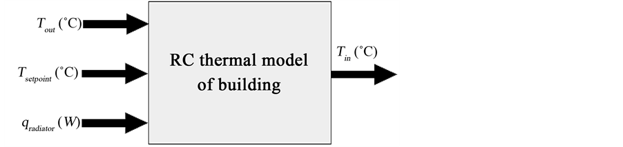
Figure 6. Building thermal model implemented using MATLAB-Simulink software.
 (8)
(8)
The resulting differential equation can be approximated by the Equation (9)
 (9)
(9)
where,  is the sampling time. We replace
  by
by , the Equation (9) becomes:
 (10)
(10)
Following in the RLS method, the error considered the total error from the measurement and estimated indoor temperature is calculated using the formula of Equation (11):
 (11)
(11)
where , is the number of measuring samples and
  is the estimated indoor temperature. We now focus our attention on sets of the parameters
  and
and  of the thermal model, which represents the weight adaptation vector taken at discrete intervals of time of Equation (10):
 (12)
(12)
where
 (13)
(13)
To adjust the weights of the adaptive linear combiner in the purpose adaptive algorithm RLS a general expression for mean square error as a function of the weight values has been given by Equation (11).
The input of RLS is given by the vector, :
:
 (14)
(14)
Which include the previous indoor temperature of moment , the heat flow from radiator at moment
  and the meteorological data of the hourly outdoor temperature at moment
  obtained in January 2013 [61] . The weight adjustment is performed during the on line training process of RLS. In this algorithm the filter weight vector is updated using Equation (15):
 (15)
(15)
 is the error between the estimated and measured indoor temperature of modeled building, and the expression of
  is given as following:
 (16)
(16)
where  is the forgetting factor between 0 and 1. By using Equations (14) and (15) can be writing as:
 (17)
(17)
The adaptation of the matrix  is given as following:
 (18)
(18)
where ,
,  is a small positive constant,
  is the identity matrix and
  is given by the Equation (14).
Finally, the filter output is calculated using the filter weights of previous iteration and the current input vector, we obtain the estimated indoor temperature of building as Equation (19):
 (19)
(19)
5.2.2. Black-Box Model
In contrast, the fact that we do not require any physical information, the black-box models compared to the grey-box methods, stay totally based on measures or empirical parameters. However, one among of different black-box tools employed to estimate and describe the indoor temperature of modeled building. We propose to use RPROP stand for “Resilient backpropagation” for artificial neural networks. The Rprop was used to perform a local adaptation of the weight-updates according to the behavior of the total squared error. To get the behavior of indoor temperature of building, we have based on [62] [63] in all our simulation of black-box and to understand the basic principle of Rprop, as described below.
1) Description of Rprop
Rprop is used to eliminate the harmful influence of the size of the partial derivative on the weight step. As a consequence, only the sign of the derivative is considered to indicate the direction of the weight update [63] . This leads to an efficient and transparent adaptation process [62] . To achieve this, we introduce for each weight its individual update-value , which solely determines the size of the weight-update. This adaptive update-value evolves during the learning process based on its local sight on the total squared error E, according to the following learning rule:
 (20)
(20)
where 
Every time the partial derivative of the corresponding weight  changes its sign. This indicates that the last update was too big and the algorithm has jumped over a local minimum. The update-value
  is decreased by the factor
 . The choice of decrease factor
  and increase factor
  0.5 and 1.2, respectively. To allow a fair comparison between the several learning procedures of artificial neural network, a wide variety of parameter values was tested for this algorithm. It use more than one parameter in which there is a lot of expense neglected that arise when searching for the other parameter values.
5.2.3. Simulation Results
In order to select a “best” model based on the test comparison by means of two suitable estimators of the behavior of the indoor temperature of modeled building. First, when grey-box is tested and RLS method is employed for the estimation of parameters. Secondly, when black-box is tested and the artificial neural networks are used for estimation of indoor temperature.
The results of simulations illustrated in Figure 7, showing the capabilities of grey-box modeling approach to capture the behavior of the indoor temperature of building obtained by means of RLS algorithm. The test, gives good tracking of the indoor temperature measured of the modeled building. The estimated parameters  and
and  observed in the graphic of the Figure 8, shows the produces significant convergence in the estimation of parameters compared with the original parameters of modeled building. Taking into account the speed of RLS technique algorithm which gives good tracking of estimation.
In on the other side in the Figure 9, show the indoor temperature of building obtained by black-box by using artificial neural network. It is clearly seen that for the case of black-box modeling approach the behavior of indoor temperature deviates from its true indoor temperature behavior. We observe an important variation in

Figure 7. Behavior of indoor temperature, obtained by grey-box model.

Figure 8. Convergence of , and
, and , obtained by means of the RLS algorithm.

Figure 9. Behavior of indoor temperature, obtained by black-box model.
comparison with the measured indoor temperature. Although a wide variety of parameter values has been used, that means that artificial neural network was not able to find the correct value of the indoor temperature. Moreover, it is the presence of the nonlinearity of the power of electric heater which complicates the behavior of indoor temperature. Whereas, with this a simple neural networks structure, we cannot remain the indoor temperature from its true behavior. On the one side, the algorithm converges considerably slowly compared to the grey-box model. But only when varying the initial parameters of the Rprop, the convergence algorithm acceleration could be changed.
6. Conclusion
In this paper, we have proposed a review of black, white and grey-boxes modeling approaches of building systems and the predictions methods enabling to improve energy efficiency of buildings. These approaches have been introduced and compared into three categories. Each of them was associated to specific paradigms and field. First approach, relying on physical models “white-box”, it is mainly correspond to a gradual rise of the level of details of building models. It is based on the laws of physics to describe the set of phenomena of residential building and to permit high fidelity modeling of the building system. Second approach, is based on observations of “black-box”, which relies on statistical and measurements treatments to describe the set of the phenomena. Those can provide little insight into the dynamics dictating the system behavior of building. It is, however, quite difficult to perform a qualitative and comparative assessment of the various techniques devised in this field. Since again their performances will depend on the training data used as input. The great power of these models is the fact that they do not need to have much knowledge on the building geometry or the detailed physical phenomena to deduce the indoor temperature. Compared to physical approaches, black-box requires less information about the building and may appear as easier to deploy. Finally, the very natural question arises, when combining between the two models to obtain a simplified model structure (grey-box) suitable for the physics principle and of the observations of phenomena of building system. Grey-box approaches appear as a very promising field for the near future. They can be appreciated in situations where a building physical model is available. Grey-box models could be of great help if there is difficult to rebuild detailed physical model.
Acknowledgements
This work was supported by Laboratoire des technologies de l’énergie (LTE) d’Hydro-Québec, Natural Science and Engineering Research Council of Canada and Fondation UQTR.
References
- Halvgaard, R., Poulsen, N.K., Madsen, H. and Jørgensen, J.B. (2012) Economic Model Predictive Control for Building Climate Control in a Smart Grid. 2012 IEEE PES Innovative Smart Grid Technologies (ISGT), Washington DC, 16-20 January 2012, 1-6. http://dx.doi.org/10.1109/ISGT.2012.6175631
- Haghighi, M.M. (2013) Controlling Energy-Efficient Buildings in the Context of Smart Grid : A Cyber Physical System Approach. Ph.D Dissertation, University of California at Berkeley, Berkeley.
- Borlase, S., Ed. (2012) Smart Grids: Infrastructure, Technology, and Solutions. CRC Press, Boca Raton.
- Zhou, Q., Wang, S.W., Xu, X.H. and Xiao, F. (2008) A Grey-Box Model of Next-Day Building Thermal Load Prediction for Energy-Efficient Control. International Journal of Energy Research, 32, 1418-1431. http://dx.doi.org/10.1002/er.1458
- Crabb, J.A, Murdoch, N. and Penman, J.M. (1987) A Simplified Thermal Response Model. Building Service Engineering Research and Technology, 8, 13-19. http://dx.doi.org/10.1177/014362448700800104
- Katipamula, S. and Brambley, M. (2005) Review Article: Methods for Fault Detection, Diagnostics, and Prognostics for Building Systems―A Review, Part II. HVAC&R Research, 11, 169-187. http://dx.doi.org/10.1080/10789669.2005.10391133
- Yang, Z.Y., Li, X.L., Tang, K., Yao, X., Bowers, C.P. and Schnier, T. (2012) An Efficient Evolutionary Approach to Parameter Identification in a Building Thermal Model. IEEE Transactions on Systems, Man, and Cybernetics, Part C: Applications and Reviews, 42, 957-969.
- Energy Solution Centre (2011) Easy$ Tip Sheets―Energy Advice Saving Yukoners Money. Energy Solution Centre Report, Whitehorse, 1-4. www.esc.gov.yk.ca
- Pouresmaeil, E., Gonzalez, J.M., Bhattacharya, K. and Canizares, C.A. (2013) Development of a Smart Residential Load Simulator for Energy Management in Smart Grids. IEEE Transactions on Power Systems, 1-8.
- Park, H., Ruellan, M., Bouvet, A., Monmasson, E. and Bennacer, R. (2011) Thermal parameter identification of simplified building model with electric appliance. 11th International Conference on Electrical Power Quality and Utilisation (EPQU), Lisbon, 17-19 October 2011, 1-6. http://dx.doi.org/10.1109/EPQU.2011.6128822
- Jiménez, M.J. and Heras, M.R. (2009) Application of Different Dynamic Analysis Approaches to Estimate the U and G Values of Building Components. Building and Environment, 44, 361-367.
- Merabtine, A. (2012) Modélisation Bond Graphs en vue de l’Efficacité Énergétique du Bâtiment. Thesis, Université de Lorraine, Lorraine.
- Zayane, C. (2011) Identification d’un modèle de comportement thermique de bâtiment à partir de sa courbe de charge. ParisTech, Paris.
- Brause, R. (2010) Adaptive Modellierung und Simulation. Rüdiger Brause, Ed., Frankfurt.
- Khan, M.E. and Farmeena, K. (2012) A Comparative Study of White Box, Black Box and Grey Box Testing Techniques. International Journal of Advanced Computer Science and Applications, 3, 12-15.
- Berthou, T., Stabat, P., Salvazet, R. and Marchio, D. (2012) Comparaison de modèles linéaires inverses pour la mise en place de stratégies d’ effacement. Rencontres AUGC-IBPSA, 1-12.
- Kawashima, M., Dorgan, C.E. and Mitchell, J.W. (1995) Hourly Thermal Load Prediction for the Next 24 Hours by ARIMA, EWMA, LR, and an Artificial Neural Network. ASHRAE Transactions, 101, 186.
- Stevenson, W.J. (1994) Predicting Building Energy Parameters Using Artificial Neural Nets. Transactions of the American Society of Heating, Refrigerating and Airconditioning Engineers, 100, 1081-1087.
- Ohlsson, M., Petersson, C., Pi, H., Rögnvaldsson, T. and Söderberg, B. (1994) Predicting System Loads with Artificial Neural Networks―Methods and Results from “The Great Energy Predictor Shootout”. ASHRAE Transactions, 100, 1063-1074.
- Feuston, B.P. and Thurtell, J.H. (1994) Generalized Nonlinear Regression with Ensemble of Neural Nets: The Great Energy Predictor Shootout. ASHRAE Transactions, 100, 1075-1080.
- Iijima, M., Takagi, K., Takeuchi, R. and Matsumoto, T. (1994) A Piecewise-Linear Regression on the ASHRAE Time- Series Data. ASHRAE Transactions, 100, 1088-1095.
- Chen, C., Wang, J., Member, S., Heo, Y. and Kishore, S. (2013) MPC-Based Appliance Scheduling for Residential Building Energy Management Controller. IEEE Transactions on Smart Grid, 4, 1401-1410.
- Szikra, C. (2014) Calculation of Heat Loss for Residential Buildings.
- Singh, R. and Vyakaranam, B. (2012) Evaluation of Representative Smart Grid Investment Grant Project Technologies: Distributed Generation. PNNL, Richland. http://www.esc.gov.yk.ca/
- Maasoumy, M., Moridian, B., Meysam, R. and Mahdi, S. (2013) Online Simultaneous State Estimation and Parameter Adaptation for Building Predictive Control. Proceedings of the ASME Dynamic Systems and Control Conference, Palo Alto, 21-23 October 2013, 1-10.
- Horváth, G. (2002) Neural Networks in System Modeling. In: Ablameyko, S., Goras, L., Gori, M. and Piuri, V., Eds., Neural Networks in Measurement Systems, IOS Press, Amsterdam, 43-78.
- Verhelst, C. (2012) Model Predictive Control of Ground Coupled Heat Pump Systems for Office Buildings. Katholieke University Leuven, Leuven.
- Christian, N., Dirk, J., Burhenne, S. and Florita, A. (2011) Modellbasierte Methoden für die Fehlererkennung und Optimierung im Gebäudebetrieb. Fraunhofer ISE, Technical Report 0327410A-C, 1-276.
- Lebrun, J. (2001) Simulation of a HVAC System with the Help of an Engineering Equation Solver Plant of an Engineering Equation Solver. Proceedings of the 7th International IBPSA Conference, Rio de Janeiro, 13-15 August 2001, 1119-1126.
- Deque, F., Ollivier, F. and Poblador, A. (2000) Grey Boxes Used to Represent Buildings with a Minimum Number of Geometric and Thermal Parameters. Energy and Buildings, 31, 29-35.
- Verhelst, C., Logist, F., Van Impe, J. and Helsen, L. (2012) Study of the Optimal Control Problem Formulation for Modulating Air-to-Water Heat Pumps Connected to a Residential Floor Heating System. Energy and Buildings, 45, 43- 53. http://dx.doi.org/10.1016/j.enbuild.2011.10.015
- Ljung, L. (2009) System Identification : Theory for the User. Prentice-Hall, Upper Saddle River.
- Tulleken, H.J.A.F. (1991) Application of the Grey-Box Approach to Parameter Estimation in Physicochemical Models. Proceedings of the 30th IEEE Conference on Decision and Control, Brighton, 11-13 December 1991, 1177-1183.
- Clarke, J.A., Cockroft, J., Conner, S., Hand, J.W., Kelly, N.J., Moore, R., O’Brien, T. and Strachan, P. (2002) Simulation-Assisted Control in Building Energy Management Systems. Energy and Buildings, 34, 933-940. http://dx.doi.org/10.1016/S0378-7788(02)00068-3
- Costanzo, G.T., Sossan, F., Marinelli, M., Bacher, P. and Madsen, H. (2013) Grey-Box Modeling for System Identification of Household Refrigerators: A Step toward Smart Appliances. Proceedings of the 4th International Youth Conference on Energy (IYCE), Siofok, 6-8 June 2013, 1-5.
- Yudong, M. (2012) Model Predictive Control for Energy Efficient Buildings. University of California, Berkeley.
- Deng, K. and Goyal, S. (2014) Structure-Preserving Model Reduction of Nonlinear Building Thermal Models. Automatica, 50, 1188-1195. http://dx.doi.org/10.1016/j.automatica.2014.02.009
- Shariatzadeh, F. and Srivastava, A.K. (2013) Look-Ahead Control Approach for Thermostatic Electric Load in Distribution System. Proceedings of the 2013 North American Power Symposium (NAPS), Manhattan, 22-24 September 2013, 1-6. http://dx.doi.org/10.1109/NAPS.2013.6666878
- Braun, J.E. (1990) Reducing Energy Costs and Peak Electrical Demand through Optimal Control of Building Thermal Storage. ASHRAE Transactions, 96, 876-888.
- Široký, J., Oldewurtel, F., Cigler, J. and Prívara, S. (2011) Experimental Analysis of Model Predictive Control for an Energy Efficient Building Heating System. Applied Energy, 88, 3079-3087. http://dx.doi.org/10.1016/j.apenergy.2011.03.009
- Verhaegen, M. and Verdult, V. (2012) Filtering and System Identification: A Least Squares Approach. Cambridge University Press, New York.
- Jan, S., Samuel, P. and Lukas, F. (2007) Model Predictive Control of Building Heating System. Energy and Buildings, 43, 564-572.
- Bohlin, P.T. (2006) Practical Grey-Box Process Identification. Springer, London.
- Peterkas, V. (1981) Bayesian System Identification. Automatica, 17, 41-53.
- Prívara, S., Siroky, J., Ferkl, L. and Cigler, J. (2011) Model Predictive Control of a Building Heating System: The First Experience. Energy and Buildings, 43, 564-572. http://dx.doi.org/10.1016/j.enbuild.2010.10.022
- Zhao, H. and Magoulès, F. (2012) A Review on the Prediction of Building Energy Consumption. Renewable and Sustainable Energy Reviews, 16, 3586-3592. http://dx.doi.org/10.1016/j.rser.2012.02.049
- McKinley, T.L. and Alleyne, A.G. (2008) Identification of Building Model Parameters and Loads Using On-Site Data Logs. Proceedings of the 3rd National Conference of IBPSA, Berkeley, 30 July-1 August 2008, 9-16.
- Bargiotas, D., Birdwell, J.D. and Ieee, S. (1988) Residential Air Conditioner Dynamic Model for Direct Load Control. IEEE Transactions on Power Delivery, 3, 2119-2126. http://dx.doi.org/10.1109/61.194024
- Chaitanya, K. (2009) Types of Heat Transfer. http://www.castilloconfort.net/bio_estufas.html
- Dewson, T., Day, B. and Irving, A.D. (1993) Least Squares Parameter Estimation of a Reduced Order Thermal Model of an Experimental Building. Building and Environment, 28, 127-137. http://dx.doi.org/10.1016/0360-1323(93)90046-6
- Taylor, Z.T., Gowri, K. and Katipamula, S. (2008) GridLAB-D Technical Support Document: Residential End-Use Module Version 1.0. PNNL-17694, Pacific Northwest National Laboratory, Richland. http://dx.doi.org/10.2172/939875
- Schneider, K.P., Member, S., Fuller, J.C. and Chassin, D.P. (2011) Multi-State Load Models for Distribution System Analysis. IEEE Transactions on Power Systems, 26, 2425-2433. http://dx.doi.org/10.1109/TPWRS.2011.2132154
- Kalsi, K., Fuller, J., Elizondo, M. and Chassin, D. (2012) Aggregate Model for Heterogeneous Thermostatically Controlled Loads with Demand Response. Proceedings of the 2012 IEEE Power and Energy Society General Meeting, San Diego, 22-26 July 2012, 1-8.
- Behl, M., Nghiem, T.X. and Mangharam, R. (2014) IMpACT : Inverse Model Accuracy and Control Performance Toolbox for Buildings. Proceedings of the 2014 IEEE International Conference on Automation Science and Engineering (CASE), Taipei, 18-22 August 2014, 1-10.
- Goyal, S. and Barooah, P. (2011) A Method for Model-Reduction of Nonlinear Building Thermal Dynamics. Proceedings of the 2011 American Control Conference (ACC), San Francisco, 29 June-1 July 2011, 2077-2082. http://dx.doi.org/10.1109/ACC.2011.5991461
- Gyalistras, D. and Division, B.T. (2010) Use of Weather and Occupancy Forecasts for Optimal Building Climate Control (OptiControl): Two Years Progress Report. ETH Zurich, Technical Report.
- Toffoli, E., Baldan, G., Albertin, G., Schenato, L., Chiuso, A. and Beghi, A. (2008) Thermodynamic Identification of Buildings Using Wireless Sensor Networks. Proceedings of the 17th IFAC World Congress, Seoul, 6-11 July 2008, 8860-8865.
- Oldewurtel, F., Sagerschnig, C. and Eva, Z. (2013) Building Modeling as a Crucial Part for Building Predictive Control. Energy and Buildings, 56, 8-22. http://dx.doi.org/10.1016/j.enbuild.2012.10.024
- Conseil National de Recherches Canada (2011) Codesnationaux. http://www.nrc-cnrc.gc.ca/fra/publications/centre_codes/codes_guides.html
- Foucquier, A., Robert, S., Suard, F., Stéphan, L. and Jay, A. (2013) State of the Art in Building Modelling and Energy Performances Prediction: A Review. Renewable and Sustainable Energy Reviews, 23, 272-288. http://dx.doi.org/10.1016/j.rser.2013.03.004
- Millette, J., Sansregret, S. and Daoud, A. (2011) SIMEB: Simplified Interface to DOE2 and Energy Plus―A User’s Perspective―Case Study of an Existing Building. Laboratory of Energy Technologies, Hydro-Québec Research Institute. Proceedings of the 12th Conference of the International Building Performance Simulation Association, Sydney, 14-16 November 2011, 2349-2355.
- Riedmiller, M. and Braun, H. (1993) A Direct Adaptive Method for Faster Backpropagation Learning: The RPROP Algorithm. Proceedings of the IEEE International Conference on Neural Networks, San Francisco, 28 March-1 April 1993, 586-591. http://dx.doi.org/10.1109/ICNN.1993.298623
- Riedmiller, M. (1994) Rprop―Description and Implementation Details. Technical Report, University of Karlsruhe, Karlsruhe.