Communications and Network
Vol.10 No.04(2018), Article ID:88300,16 pages
10.4236/cn.2018.104015
Performance Comparison and Simulink Model of Firewall Free BSD and Linux
Fontaine Rafamantanantsoa*, Haja Louis Rabetafika
University of Fianarantsoa, Fianarantsoa, Madagascar

Copyright © 2018 by authors and Scientific Research Publishing Inc.
This work is licensed under the Creative Commons Attribution International License (CC BY 4.0).
http://creativecommons.org/licenses/by/4.0/


Received: July 27, 2018; Accepted: November 3, 2018; Published: November 5, 2018
ABSTRACT
In recent years, the number of users connected to the Internet has experienced a phenomenal growth. The security of systems and networks become essential. That is why the performance of Linux firewall and Berkeley Software Distribution (BSD) are of paramount importance in security systems and networks in all businesses. The following evaluates the firewall based tool that we have developed in Python and Scapy, which performs time measurements by serving packets traversing the firewall test. Several results were presented: the speed of the firewall under FreeBSD in terms of service time compared to the speed of the firewall under Linux as the number of rules increases; the speed of the filtering rule of a firewall stateless in terms of service time compared to the filtering rule of an active firewall gradually as the number of rules increases. Then, for care of simplicity, we have presented the queue M/M/1/K to model the performances of firewalls. The resulting model was validated using Simulink and mean squared error. The analytical model and Simulink of the firewalls are presented in the article.
Keywords:
Firewall, Ipfw, Iptables, Python, Scapy, Simulink, Statefull Firewall, Stateless Firewall

1. Introduction
The Web has become increasingly popular. The number of Internet users continues to increase; therefore the number of malicious sources and hacking becomes significant. That is why firewalls such as IP cop Linux and BSD PF sense are of paramount importance.
Various studies [1] [2] [3] proposed modeling, analysis, simulation and management of firewall policy; the work [4] [5] [6] presented designs, implementations firewall with software and hardware tools. [7] - [16] studied firewall filtering management and classifying packets in a secure architecture. In this paper there is a presentation tool which was developed in python and Scapy 2.2.0. Its interface was performed with Qt4 designer to measure the performance of the firewall. There is also the presentation of the model in Simulink.
Optimization settings of the operating system and firewall are solutions to improve performance. This task is not easy because the optimum values of these parameters vary depending on hardware configurations and the law of the requested service to the firewall.
This paper being divided into 4 sections, we will evaluate and model the performance of the firewall. In Section 1 we present the performance of the firewall. Configuration experiments and experimental results of firewalls will be considered respectively in Section 2 and 3. A simple model to represent the behavior of a firewall will be given at the end of the article.
2. Performance of Firewall
A firewall is a device used to prevent unauthorized access to network.
To properly evaluate the performances of a firewall, the system must meet the following conditions:
• A computer on which the firewallis settled.
• A client machine that is the tool for performance measurement that was developed in Python and Scapy.
• A network connecting the firewall and the client machine
Five metrics are used to measure the ability of the firewall:
• The number of requests processed per second is a measure of the number of requests set by the tool Scapy for a period of time.
• The size of the packet to be sent to the firewall is set to 512 bytes equal to the size of the Ethernet frame.
• The number of rules attached to the firewall.
• The status of the firewall that is stateless or has a state.
• Access in terms of rank in the firewall rule.
2.1. Methodology for Performance Analysis
The main steps for performance evaluation are:
• Sending packets to the firewall by specifying metrics.
From the Scapytool, we send the packets from the computer with two network cards connected to a network with the firewall which also has two network cards ensuring the return packets are synchronized by the clock between machines.
• Analysis of the pcap file generated by the sending packet.
• From the written paper to the pcap data, we get the time departures and arrivals of packets.
• Analysis of the performance of the firewall.
We calculate the service time E[S] is sending the packet. We compare the speed of sending time for each metric.
Figure 1 shows the experimental configuration.
Figure 1 shows that the time E[S] is the mean service time for a request as the packet traverses the firewall. E[S] can be calculated by subtracting the time between output and input firewall packet time. Packets are sent from the machine where the benchmark is installed i.e. where the tool developed in python and Scapy is installed. The machine has an IP address 172.16.1.230 with the first network card for the firewall and the first network card having an IP address 172.16.1.232. After arriving at its firewall the packages will be returned via the second network card with an IP address 172.16.2.232. The firewall on the machine where the benchmark is set by the second network card with an IP address 172.16.2.229 is to ensure clock synchronization between the machines. Access to the firewall rule in terms of rank is the last rule of each measure.
2.2. Architecture of Firewall
The function of the firewall is twofold: to strengthen security policy and log network traffic. Strengthening of a security policy based on whether to accept or reject a connection based on specific filtering rules to force a network to comply with a given policy. Logging in turn, is to record all aspects of trafficking in order to better analyze results. A firewall is a key component in designing a secure network.
However, being a transit point for all network traffic, a firewall can also be a single point of failure. Therefore, its choice and its location are import tasks for securing network infrastructures.
Figure 2 shows the architecture of firewall considered.
3. Configuring Experiments
The characteristics of the test system used are shown in Table 1.
Table 1 summarizes the hardware and software used for the experiments. FreeBSD 9.0 was installed in dual boot on the same machine without any hardware modification with Ubuntu 13.10 operating system using the last version 1.4.18 IP tables.
To obtain reliable results, each experiment was launched for five minutes.
E[S] is the service time of the packet passing through the firewall.

Table 1. Characteristics of hardware and software used in the experiments.

Figure 1. Experimental configuration.

Figure 2. Architecture of firewall.
3.1. Presentation of the Measurement Tool
Python is an object-language, multi-paradigm and multi-platform programming. It promotes structured imperative and object-oriented programming.
Scapy is a free software for handling network packets written in python language.
Qt (pronounced officially cute in English (/kju: t/) commonly but mistakenly pronounced QT) is:
• Object-oriented and developed in C++ Qt Development Framworks, a subsidiary of Digia PLC.
• In some ways a framework when used for designing graphical user interfaces or in the application architecture using the mechanisms of signals and slots for example.
We developed in python and Scapy 2.2.0 and its interface was made with Qt4 Designer. This tool sends packets from the machine tool with the python Scapy through the firewall and back to the machine tool with the python Scapy, on arrival at the source host through the second network card to ensure the clock synchronization.
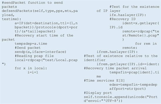
3.2. Extracted from Source Code
4. Experimental Results Firewall
A series of experiments were conducted to examine the performance of the firewall.
Taking measures to assess performance, varying the number of rules and the rank of the rule for the firewall, we performed measurements with UDP and TCP protocols. First, all access has been granted, i.e. the chain input, output and transfer to the firewall are open. After the input and output channels were closed, but the transfer line remained open.
We conclude that success to cross the firewall depends on the chain transfer even if the input and output channels are closed.
The Matlab tool was used for the activities of modeling, curves and comparison with firewalls and stateless firewalls; in particular depending on the number of rules using both TCP and UDP protocols.
Figure 3 shows a graphic interface of the tool for measuring the performance of the firewall.
Description of the Measurement Tool
1) This is the text area of the destination IP address that is the IP of the firewall where packets are sent. Radio buttons are used to check the exact type of protocol used.
2) This is the text area of the port used by the tool when sending the packets.
3) This is the text area of the number of rules attached to the firewall that are automatically generated by the tool.
4) This is the text area of the number of requests sent per second; its requests will be sent to the firewall.
5) This is the text area for the second period of the experiment. Here it is five minutes.

Figure 3. Graphical interface tool for measuring the performance of the firewall.
6) This is the text area of the size in bytes of the packet sent. Here it is set to 512 bytes equal to the size of the Ethernet frame.
7) This is the text area of the rank of the rules to the firewall.
8) This is the display area of the result of the experiment as the time of service obtained is displayed, as well as times of departures and arrivals of packets. The start button is used to start the measurement after the text boxes are filled.
The stop button is used to stop the measure during launch.
The curve button is used to display the curve representative of the service time E[S] based on the number of rules to the firewall.
Table 2 shows the service time E[S] as a function of number of rules under FreeBSD and Linux using TCP.
Figure 4 shows the curve of the service time E[S] as a function of number of rules under FreeBSD and Linux using TCP.
Figure 4 shows that FreeBSD and Linux using TCP, the average service time request protocol for E[S] as a function of the number of rules slowed gradually as the function of the rules increases. This can be explained by the slowdown in service time caused by the increase in number of rules caused by the increase in access to the rules of the firewall time.
The formula of the curve of the service time E[S] as a function of number of rules in FreeBSD using TCP Matlab is given by:
The formula of the curve of the service time E[S] as a function of the number of rules under Linux using TCP Matlab is given by:
Table 3 shows the service time E[S] as a function of the number of rules under FreeBSD and Linux using the UDP protocol.
Figure 5 shows the curve of the service time E[S] as a function of the number of rules under FreeBSD and Linux using the UDP protocol.
Figure 5 shows that FreeBSD and Linux using UDP, the average service time request protocol for E[S] as a function of the number of rules slowed gradually as the number of rules increases. This can be explained by the increase of the rules caused by the increase in access time to the rules of the firewall.
The formula for the curve of the service time E[S] as a function of the number of rules in FreeBSD using UDP Matlab is given by:
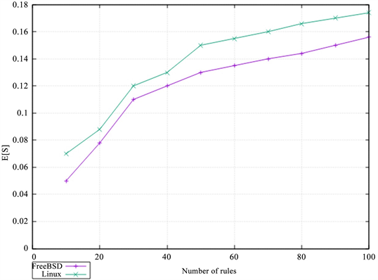
Figure 4. Curve service time E[S] as a function of number of rules under FreeBSD and Linux using TCP.

Figure 5. Curve service time E[S] as a function of number of rules under FreeBSD and Linux using UDP.
Table 2. Service time E[S] as a function of number of rules under FreeBSD and Linux using TCP.
Table 3. Service time E[S] as a function of number of rules under FreeBSD and Linux using UDP.
The formula for the curve of the service time E[S] as a function of the number of rules under Linux using the UDP protocol Matlab is given by:
We can conclude that its figures service time E[S] with FreeBSD is faster than service time E[S] under Ubuntu. So the firewall FreeBSD is faster than Ubuntu Linux firewall.
Table 4 shows the filtering rule of stateless firewalls and stateful firewalls, service time E[S] as a function of the number of rules.
Figure 6 shows the curve of the filtering rule firewall stateless and statefull firewall, service time E[S] based on the number of rules.
Figure 6 shows the rule with the filtering stateless firewall and statefull firewall, the average service time for a request E[S] as a function of number of rules gradually slowed. This can be explained by the slowdown in service time caused by the increase in access to the rules of the firewall time.
The formula for the curve of the filtering rule of stateless firewall with Matlab is given by:
Table 4. Rule filtering firewall stateless and stateful firewall, service time E[S] as a function of number of rules.

Figure 6. Curve rule filtering firewall stateless and statefull.
The formula for the curve of the filtering rule of statefull firewall with Matlab is given by:
We conclude by these figures that the rule of filtering stateless firewalls is faster in terms of service time compared to the filtering rule statefull firewalls. This speed in time of stateless firewall is relative to the statefull firewalls due verification packets to a connection over it. That is to say, they check that each packet of a connection is the result of the previous packet in the other direction; whereas with stateless firewalls, it looks at each packet independently of the others and compared to a list of preconfigured rules.
5. Analytical Model Firewall
For a period of five minutes the simulation, we obtain this model.
By analyzing data from the log files located in /var/log firewall University of Fianarantsoa at the National School of Computer Science, that is to say by importing data with the software located in Matlab script, this software gives an average value of the number of requests per second λ 100, we conclude that the arrival traffic follows the law of Poisson, the number of objects used in a given period is exponential, number of firewall is 1 and the length of the queue is a fixed constant.
We see that with the number of requests per second 100, the firewall at the University of Fianarantsoa in the National School of Computer does not choke. So the queue type: M/M/1/K.
λ: Arrival rate;
µ: Service rate.
Define the traffic intensity (Traffic Intensity) or occupancy rate ρ server (rho) by:
When a customer arrives when there is already a k customers in the system.
The queue is stable without condition.
p(n): stationary probability;
k: capacity of the line, either waiting or in service;
n = 0, …, k.
Finally .
The service takes place with a rate in each state where the system contains at least one client
The utilization rate is the probability that the server of the queue is busy:
Average Customer Q
Average residence time R
6. Simulation with Matlab
By varying the length of the wire waiting 10 to 2000 with a default length of the firewall equal to 1000, we also vary from 20 to 120 the number of requests sent per second λ for each length of wire waiting in the block Event-Based Random Number. Here is the exponential distribution, to each value of λ for a length of thread waiting we run the Simulink model for 5 minutes and we got the curves of the simulation. After we pooled data obtained from all the values of λ for a length of wire waiting and we got the final curve.
Figure 7 shows the model in Simulink.
In this Figure 7, the bloc Event-Based Random Number generates in a random manner based on a number events. It generates a new random number each time an entity arrival on the server occurs. Here is the exponential distribution,
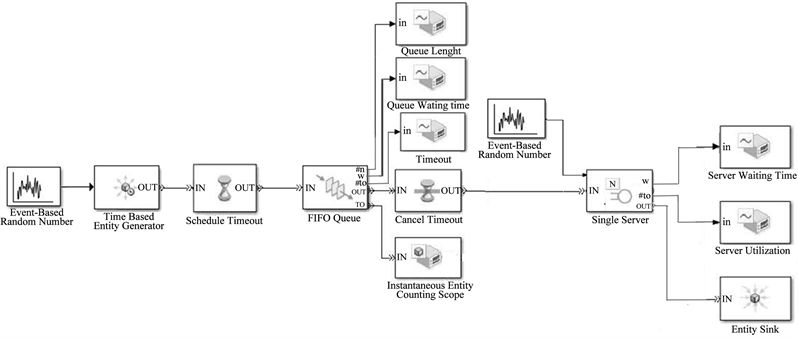
Figure 7. Model Simulink.
the mean value is equal to where λ is the number of requests sent per second we ranged from 20 to 120. T after the port, there our binding block Time-Based entity Generator is designed to generate entities that meet the criteria that we specify. The inter-generation time is the time interval between two successive events of generation. After the IN port, it will link to the Schedule Timeout block which determines a timer event for each entity arrival. This block refers to a beginning of a path of the entity that is relevant to the time. After the IN port, it will link to the block FIFO queue which is a first in, first out queue that’s length was varied from 10 to 2000 by the input sequence. Port #n, w, #to, TO are respectively related to scope, Queue Length signal which shows the curve length of the queue, Queue waiting time witch shows the curve of latency queue, Timeout which shows the flow curve and Instantaneous Entity counting scope that shows the curve of the number of packets waiting.
After the IN port, it will block binding Cancel Timeout cancels an expiration event name as the block timing schedule previously provided to the entity arrival. It allows us to limit the time that the entity passes along the paths of the entity designated in the simulation. This means it blocks one end of a path of an entity that is relevant for the time. The possibility of canceling event timeout before they occur allows us to apply the time an entity path. After the IN port, it will link to the Single Server block which represents the firewall in our case and ports w and util are linked respectively to signal scope server utilization which shows the curve using the server, the server waiting time which shows the latency server, port t is related to the block Event-Based Random Number, by the mean value is equal to the average value of E[S]. After the IN port, it will link to the Entity Sink block which provides a way to end a path entity.
Table 5 shows the use of the server.
For the length of queue equal to 1000 we got the following lines: Figure 8 shows the curve of server usage.
6.1. Resolution of the Mean Squared Error
The mean squared error is a measure of the average error, weighted by the square of the error. It answers the question, “what is the magnitude of the error of prediction”, but does not indicate the direction of errors. Because it is a quantity in square, the square error is influenced more by large errors than smaller errors. Its range is 0 to infinity, a score of 0 being a perfect score.
Here the mean squared error represents the difference between the curve of the model and the measured curve.
where Fi = the prediction values of the parameter;
Oi = the value corresponding verification (observed or analyzed);
N = the number of check points (grid points or observation points) in the verification area.

Figure 8. Server utilization curve.
Table 5. Use server.
6.2. Calculating the Mean Squared Error Using the Server
MSE = 0.00682.
The mean squared error of the server utilization is very low, therefore the model curve of the measured curve and the use of the server are similar.
Curve using the server shows that there is strong growth until congestion firewall and reach the maximum value equal to 1 because the number of treatments increases and at the time of congestion firewall curve becomes constant.
This can be explained by the increased length of the queue causes the late arrival of rejection according to the number of requests per second since the processing queue is long and the length of the queue decreases, the arrival of rejection is advanced according to the number of requests per second for processing the queue is short.
Table 6 shows the throughput according to the number of requests per second.
Figure 9 shows the flow curve as a function of the number of requests per second.
Table 6. Table flow.

Figure 9. Flow curve based on the number of requests per second.
6.3. Calculating the Mean Squared Error Rates
where
Fi = the prediction values of the parameter;
Oi = the value corresponding verification (observed or analyzed);
N = the number of check points (grid points or observation points) in the verification area.
MSE = 0.00682.
The mean squared error rates are very low; therefore the model curve and the measured curve rates are similar.
The rate curve shows that there are growing rates according to the length of the queue until the arrival of rejection. And when the rejection rate curve decreases, it can be explained by the rejection of the firewall to check for rejection. If the length of the queue increases, the arrival of the discharge is delayed according to the number of requests per second. If the processing queue is long and if the length of the queue decreases, the arrival of rejection is advanced according to the number of requests per second for processing the queue is short.
We can conclude that in terms of resources if the length of the queue increases the percentage of the Central Processing Unit (CPU) used increases, this can be explained by the growth of treatment until the arrival of rejection and decrease in the length of the queue causes the decrease in the percentage of CPU used compared to high waiting queue, this can be explained by the decrease in treatment until the arrival of rejection.
We set the default length of the queue to 1000.
7. Conclusion
This paper presented the performance evaluation and modeling of a firewall. In Section 1 we presented the performance of the firewall. Configurations, experiments and experimental results of the firewall are examined respectively in Sections 2 and 3. A simple mode which represented the behavior of a firewall is given at the end of the article. We developed a tool in python and Scapy 2.2.0 and its interface has been achieved with Qt4 designer which sent packets from the machine through the firewall and back to the machine with the Python Scapytool. On arrival at the firewall, packets are sent to the source host through the second network card to ensure clock synchronization. Our measurements have led us to conclude that the filtering rule of stateless firewall is faster in terms of service time compared to the filtering rule of statefull firewall. We compared two filtering rules as they are increasingly implemented on the firewall. The mean squared errors are very low so the curves are similar. Our measurements have also led us to conclude that the firewall FreeBSD is faster in terms of service time compared to the for Linux firewall.
Conflicts of Interest
The authors declare no conflicts of interest regarding the publication of this paper.
Cite this paper
Rafamantanantsoa, F. and Rabetafika, H.L. (2018) Performance Comparison and Simulink Model of Firewall Free BSD and Linux. Communications and Network, 10, 180-195. https://doi.org/10.4236/cn.2018.104015
References
- 1. Al-Shaer, E. and Hamed, H. (2004) Modeling and Management of Firewall Policies. IEEE Transactions on Network and Service Management, 1, 2-10.
- 2. Fulp, E.W. (2005) Optimization of Network Firewalls Policies Using Directed Acyclic graphs. Proceedings of the IEEE Internet Management Conference, Wake Forest University, 1-2.
- 3. Zaliva, V. (2008) Firewall Policy Modeling, Analysis and Simulation: A Survey Source-Forge. Tech Rep.
- 4. Wagner, A. and Consecom, A.G. (2012) Firewall Analysis by Symbolic Simulation, Bern University of Applied Sciences, Biel Switzerland. Ulrich Fiedler, Berlin, Zurich.
- 5. Schuba, C.L. (1997) On the Modeling, Design, and Implementation of Firewall Technology. Purdue University, West Lafayette.
- 6. Qui, L.L., Varghese, G. and Suri, S. (2001) Fast Firewall Implementations for Software and Hardware-Based Routers. Proceedings Ninth International Conference on Network Protocols, ICNP 2001, Riverside, 11-14 November 2001.
- 7. Srinivasan, V., Suri, S. and Varghese, G. (1999) Packet Classification Using Tuple Space Search. Computer ACM SIGCOMM Communication Review.
- 8. Al-Shaer E.S., Woo, T., et al. (2004) Modeling and Management of Firewall Policies. IEEE Transactions on Network and Service Management, 1, 2-10.
- 9. Eppstein, D. and Muthukrishnan, S. (2001) Internet Packet Filter Management and Rectangle Geometry. Proceedings of the Twelfth Annual ACM-SIAM Symposium on Discrete Algorithms, Washington DC, 7-9 January 2001, 827-835.
- 10. Hari, B., Suri, S. and Parulkar, G. (2000) Detecting and Resolving Packet Filter Conflicts. Proceedings IEEE INFOCOM 2000 Conference on Computer Communications, Tel Aviv, 26-30 March 2000.
- 11. Atkinson, R. (1995) RFC-1825 Security Architecture for the Internet Protocol. Network Working Group.
- 12. Avolio, F.M. and Ranum, M.J. (1994) A Network Perimeter with Secure External Access. Internet Society (ISOC).
- 13. Al-Shaer, E. and Hamed, H. (2002) Design and Implementation of Firewall Policy Advisor Tools.
- 14. Bartal, Y., Mayer, A., Nissim, K. and Wool, A. (1999) Firmato: A Novel Firewall Management Toolkit. Proceedings of the 1999 IEEE Symposium on Security and Privacy, Oaklan, 6 August 2002, 3-4.
- 15. Chapman, D. and Zwicky, E. (2000) Building Internet Firewalls. 2nd Edition, Orielly & Associates Inc., Newton.
- 16. Cheswick, W. and Belovin, S. (1995) Firewalls and Internet Security. Addison-Wesley, Boston.