Advances in Pure Mathematics
Vol.05 No.11(2015), Article ID:59830,14 pages
10.4236/apm.2015.511063
Sine-Generated Curves: Theoretical and Empirical Notes
Dean Hathout
Flintridge Preparatory School, La Canada, CA, USA
Email: dhathout@aol.com
Copyright © 2015 by author and Scientific Research Publishing Inc.
This work is licensed under the Creative Commons Attribution International License (CC BY).
http://creativecommons.org/licenses/by/4.0/


Received 26 August 2015; accepted 20 September 2015; published 23 September 2015
ABSTRACT
Sine-generated curves belong to a class of intrinsic functions which describe a curve by specifying its “direction angle”. The curve is determined by ω, the maximum angle which the curve makes with the horizontal, and the fact that the direction angle changes in a sinusoidal fashion along the path. Sine-generated curves are shown to be excellent approximations to the path of minimal average curvature, and expressions for radius of curvature and curve sinuosity are derived.
Keywords:
Parametric Curves, Calculus of Variations, Optimization

1. Introduction
This paper will examine, both theoretically and empirically, various aspects of a family of parametric curves known as sine-generated curves. These curves arise most naturally in geophysics in the study of meandering structures such as rivers [1] [2] , but can be studied quite abstractly. Sine-generated curves belong to a class of intrinsic functions which describe a curve by specifying its “direction angle,”; i.e. by describing how the direction of the curve changes in terms of the angle it makes with respect to the horizontal at each point along its path. For the sine-generated curve, the direction angle of the curve,  , varies in a sinusoidal fashion along the length of the curve. It is important to stress that such a curve is not a sine curve, wherein the curve itself is sinusoidal. Rather, for a sine-generated curve, the direction angle of the curve, as a function of distance along the curve, varies in a sinusoidal fashion. The curve is defined by ω, the maximum angle which the curve makes with
the horizontal. Specifically, 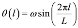 , where L is the curve length from trough to trough. Since θ de-
fines the direction of the curve at each point,
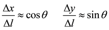
where  is the distance moved along the path. If we take the limit for
 , then
 (1a)
(1a)
 (1b)
(1b)
These equations are satisfied by each value l in 0 < l < L. We can see that when the value of l changes, the values of x, y, and θ will change in response and so we can think of x, y, and θ as functions of l. To find functions for x and y, we can integrate the two above equations with respect to l.
The sine generated curve is then described parametrically by:
 (2a)
(2a)
 (2b)
(2b)
where t varies across the curve length from 0 to L.
Sine generated curves are of interest in that they provide a convenient closed-form approximation to the curve which has the least average curvature per unit length. In other words, the curve which, as it meanders between two points, A and B, provides the minimum changes in direction for a particle traveling along the curve. This would, for example, minimize the energy needed to accelerate the particle (by changing its direction) through a curved path. Of course, the absolute minimum change in direction would be a straight line segment between points A and B. We assume that our curves deviate from this straight-line course, and take instead a winding, curved path. The question is then to specify the shape of this curve according to the optimality criterion presented above. As noted above, these curves have been analyzed in the setting of river meanders, where the curvature of rivers seems to follow the trajectory of sine-generated curves. This analysis has been undertaken mainly by Leopold and Langbein [1] [2] . A variant analysis was also introduced by Adam [3] . A more detailed theoretical derivation of sine-gen- erated curves, as well as the notion of empiric testing of these curves, was introduced by Movshovitz-Hadar and Shmukler [4] . An alternative derivation of the differential equation leading to sine-generated curves, based on a random walk analysis of particle paths, was performed by Von Schelling [5] .
This paper will present a more direct derivation of sine-generated curves as curves of minimal average curvature, similar to that offered by Adam [3] , who dealt instead with cosine-generated curves. The paper will then empirically test sine-generated curves against similar curves to help confirm that they are good approximations to paths of minimal average curvature. The main parameters of interest in these curves will be the path length L of a particle flowing along the curved segment as defined above, the “wavelength” Lx, defined as in a cosine or sine wave as horizontal distance along the x-axis from trough to trough, and the radius of curvature R, which defines the radius of a circle which has as its arc the peak of the curve. To normalize for the effect of curve length, and give dimensionless numbers which can be compared between curves, these parameters are combined into two ratios,  , and
, and , which characterize curvature. The latter ratio,
  , is known as the sinuosity of a curve, which will be termed s. (See Figure 1).
After empirically examining these parameters of interest, theoretical derivations of simplified expressions for , and
, and  will be presented. Of particular interest is that sinuosity, or
 , can be represented in terms of a Bessel function. This derivation was apparently not available in the early analyses of sine-generated curves, where various authors such as Leoplod and Langbein [1] [2] derived only an empirical relationship by curve fitting. Interesting aspects of the derivations, such as the Euler-Lagrange equation from the calculus of variations, will be presented in a separate appendix.
2. Derivation of the Sine-Generated Function
Let the curvature of a curve be defined as . Then, we consider the mean squared curvature to be defined by

Figure 1. The parameters of interest in analyzing tortuosity. L is arc length along the curve between A and B, Lx represents the horizontal wavelength between A and B, and R represents the radius of curvature. The maximal direction angle is ω, which is considered as a given in the specification of a sine-generated curve.
 (3)
(3)
From the above, we are looking for the curve with minimal changes in direction, and so we will require the mean squared derivative of the curvature to be a minimum, as this would be one way to minimize the energy
required for turning. Therefore, we are looking for curves which, for a given average curvature , minimize
 (4)
(4)
To find curves which minimize Equation (4) subject to the constraint of Equation (3), we will follow lines similar to Adam [3] . We begin with non-dimensionalization of Equation (3) and Equation (4) to simplify the subsequent analysis. We can begin by defining  and
and . With these definitions, Equation (3) and Equation (4) may then be re-expressed as
 (5)
(5)
 (6)
(6)
Now, the integrals are with respect to the normalized path length , and hence the integration limits are 0 and 1.
The problem now becomes to minimize the integral of Equation (6) subject to the constraint of Equation (5). This is an isoperimetric problem, and can be solved by introducing a Lagrange multiplier λ into a calculus of variations formulation, and form a new functional  whose integral we wish to minimize:
 (7)
(7)
Here, we know the form of , and we wish to find the
  which minimizes the integral in Equation (7). When this is found, it is defined to be the form which minimizes the derivative of the direction angle with
respect to normalized motion along the curve , i.e., the minimum change of direction angle.
To find the desired function, we introduce a theorem from the calculus of variations that  must satisfy the Euler-Lagrange equation:
 (8)
(8)
Given the centrality of this equation to the exposition, it is derived in Appendix A.
Upon substituting  into Equation (8), we get a simple second-order differential equation,
 (9)
(9)
The general solution to this equation is
 (10)
(10)
By direct integration, we then get
 (11)
(11)
Here,  and
and  are constants, as is λ. Looking at the form of the sine-generated curve gives us the needed reasonable boundary conditions to determine these constants. We see that the curve is flat at
  and at
 , i.e., at the apex of the curve. Also, the maximal direction angle is reached when
 . Therefore, our boundary conditions become θ = 0 at
 ,
,  at
at , and
, and  at
at . These boundary conditions give
us ,
,  and
and . Therefore,
  , and remembering that
 , we get
 .
.
A less direct, but perhaps more interesting, derivation of the sine-generated curve begins with a different definition of average curvature [4] . In this case, the average curvature,  , is defined as the integral square average of
 :
:
 (12)
(12)
In this case, the problem becomes to minimize the integral:
 . (13)
Similar to the above, the problem can be tackled through the calculus of variations [4] , and the result is an integral equation which implicitly specifies ,
,
 (14)
(14)
where α is a constant, ω is the maximal direction angle as defined previously, and where θ implies .
.
Although this integral has no closed form solution, it can be shown that  provides a good approximate closed-form solution [4] .
The reason this derivation is of interest is that Equation (13) results naturally from a probabilistic approach to the mathematical modeling of particle paths. If a particle takes a random walk from point A to point B in a fixed number of steps, able to change its direction at random at each step, it is possible to search for the most probable resulting curve, which leads to a path defined by minimizing Equation (13) ( [5] , Appendix B). Thus, the sine- generated curve represents a good closed-form approximation to the most probable path taken by a particle undergoing a random walk of fixed length.
3. Empiric Testing of the Sine-Generated Curve
As noted above, the intrinsic form of the sine-generated curve,  , represents an infinite family
of curves, each specified by the value of ω. Each different value of ω produces a unique sine-generated curve. Any curve of this family can be transformed into a set of parametric equations which represent the curve conventionally on Cartesian coordinates (Equations (2a), (2b))
These curves are rendered using numerical integration, assuming a path length (L) of 10. We see that the shape of the sine-generated curve will be essentially uniquely determined by ω. Figure 2 shows the appearance of the sine-generated curves for several values of ω.
Because of the well-known approximation that  for small values of θ, the sine-generated curve can be approximated by a sine (or cosine) curve for small values of ω. For larger values, however, there is a significant deviation in shape, with the sine-generated curve appearing “rounder,” with a more gentle curvature (see Figure 3).
One interesting result of the sine-generated curve model is that it generates loops for values of ω above approximately 126˚ (see Figure 4), which sinusoids do not do.
The sine-generated curve should be the curve of minimum average curvature (i.e., minimum changes of direction). It is worth empirically verifying this proposition in comparison to some “reasonable” curves which have a similar appearance. Returning to Equation (12), average curvature per unit length for the sine-generated curve can now be rewritten as:
 (15)
(15)
Average curvature is calculated using numerical integration of Equation (15).

Figure 2. (a)-(d): Sine-generated curves for ω expressed in degrees. ω = 20˚ (a), 40˚ (b), 60˚ (c) and 90˚ (d). It is noted that sinuosity (the ratio L/Lx) increases with increasing ω.
 (a) (b)
Figure 3. (a)-(b). Sine-generated curve (blue) with a sine curve (green) normalized to the same peak and same wavelength for comparison. (a) ω = 30˚; the curves are essentially identical. (b) ω = 70˚. There is a significant difference in curve shape.

Figure 4. Sine-generated curve with ω = 140˚ shows the curve looping on itself.
In Figure 5, a sine-generated curve is graphed along with a sine curve of matching wavelength and amplitude. The calculated average curvature per unit length for the sine-generated curve is 0.54, while for the sine curve, it is 0.59.
A more difficult challenge is to test the sine-generated curve against a curve specifically designed to approxi-
mate its shape. The sine-generated curve is specified intrinsically as per Equation (2), with .
.
We note that , the direction function, has a maximum value of ω, and goes to zero at the values of l = 0,
l = L, and l = L/2. We construct a similar function,  as follows:
 . This has the same
zeros as . The derivative of
  is
is . We note that
  for
for . It turns out that
  reaches a maximum at
 . We can designate the absolute value of this maxi-
mum as . Now, we can define a new direction function as

Figure 5. Sine-generated curve with ω = 70˚, L = 10, plotted with a sine curve normalized to the same amplitude and wavelength. The calculated average curvature per unit length for the sine-generated curve is 0.54, while for the sine curve, it is 0.59.
 . (16)
This has the same maximum and the same zeros as , and can serve as the direction function for a new curve, which we will term the spline curve, which can be defined parametrically as:
 (17a)
(17a)
 (17b)
(17b)
Figure 6 shows the sine-generated curve graphed along with the spline curve defined by Equations (16) and (17).
The curves are extremely similar in appearance, as they must be, given the similarity of their direction functions. The average curvature per unit length of the sine-generated curve is 0.468, while that of the spline curve is 0.489. This helps support the argument that the sine-generated curve represents a curve of minimal average curvature.
It is also instructive to investigate  empirically, since it easily obtained as part of the programming of the curves. It is noted that the choice of L = 10 is simply a scaling factor, and does not affect the ratios
  and
and .
.
By studying these parameters across multiple values of ω, it is possible to obtain an empirical equation which provides a good fit for the relationship of s to ω. With ω expressed in radians, we note that
 (18)
(18)
Figure 7 shows a graph of this function against the actual values of (ω,s) calculated from the sine-generated curves. It is noted that this empirical relationship provides an excellent fit for the sinuosity of sine-generated curves over the range of ω relevant for many practical applications, from 0˚ to 90˚.
Having established a valid relationship, we can solve for s in Equation (18) to produce the following:
 (19)
(19)
It is noted that  and
and  vary directly with ω. For smaller values of ω, the curve is less steep, and hence the radius of curvature is bigger. Thus, both L/R and
  are smaller for smaller ω (Figure 8).

Figure 6. The sine-generated curve (blue) is plotted along with the spline curve (green), showing their extreme similarity in shape. ω = 60˚, L = 10. The average curvature per unit length of the sine- generated curve is 0.468, while that of the spline curve is 0.489.

Figure 7. A scatter plot of ω (y-axis) versus s (sinuosity, L/Lx) for sine-generated curves with ω expressed in radians. The range of 0 - 1.6 radians is equivalent to approximately 0˚ - 90˚. This is overlain by a plot of Equation (18), . The plots demonstrate an excellent fir of this equation to the data from the sine- generated curves.
4. Deriving the Curvature Properties L/R, and L/Lx
These empirical results motivate a further theoretical exploration of parameters of interest for sine-generated curves.
As specified above in Equation (2), the sine generated curve is described parametrically by:


According to a well-known result from calculus, for a parametric curve, the radius of curvature R(t) along any point on the curve is given by:
 (a) (b)
Figure 8. (a)-(b): Sine-generated curves for ω = 30˚. (a) and 60˚ (b). For ω = 30˚, L/Lx = 1.07 and L/R = 3.29. For ω = 60˚, L/Lx = 1.34, and L/R = 6.58, both larger for larger ω. As can be seen, with smaller ω, there is a significantly larger radius of curvature.
 (20)
(20)
Now, we let ω be specified in radians as , and calculate
 . Since
  is an integral, this implies taking the derivative of an integral, and requires the use of Leibniz’s integral formula.
Thus, .
.
Similarly, .
.
From here, it is straightforward to calculate  and
and :
:

Plugging these expressions into Equation (20) for curvature above, we get (after some algebra):
 (21)
(21)
Our interest lies in the radius of curvature of the apex of the sine generated curve, i.e., where t = L/2. Plugging this into the above equation and taking the absolute value, we get:
 , for the radius of curvature of our sine-generated curve.
Since ω is specified in radians as , we have
 . Thus, we have
 .
.
We are interested in the parameter L/R, which has the remarkably simple and elegant expression:
 . (22)
Next, we can turn our attention to investigating , again following lines similar to Adam [3] . Once
again, starting with , and recalling that
 , we can say that
 . Recalling that
 , we can say that
 (23)
(23)
Now, recalling Equation (1a), that , we state that
 , and recalling that
 , we
, we
have . Also, we recall that
 . From these relationships, it follows that
 (24)
(24)
Now, substituting Equation (23) into Equation (24), we can state that
 (25)
(25)
Now, we can integrate both sides. The differential on the left is a differential of a normalized length, like . If we integrate the differential element on the left from 0 to 1/4, and recall our boundary conditions
  at
at  and
and  at
at , we can write:
 .
.
Now, if we let , we can say that
 (26)
(26)
This integral is quite significant, since it is essentially a Bessel function. It is shown in a variety of sources [6] that , the Bessel function of the first kind of order zero, can be expressed as
 .
.
Therefore, from Equation (26), it follows directly that
 (27)
(27)
This theoretical result is valid up to the first zero of the Bessel function at , and is an excellent match for the empirical result of Equation (19).
Cite this paper
Dean Hathout, (2015) Sine-Generated Curves: Theoretical and Empirical Notes. Advances in Pure Mathematics,05,689-702. doi: 10.4236/apm.2015.511063
References
- 1. Leopold, L.B. and Langbein, W.B. (1966) River Meanders. Scientific American, 214, 60-70.
http://dx.doi.org/10.1038/scientificamerican0666-60 - 2. Langbein, W.B. and Leopold, L.B. (1966) River Meanders: Theory of Minimum Variance. US Geological Survey Professional Paper 422-H.
- 3. Adam, J. (2006) Mathematics in Nature: Modeling Patterns in the Natural World. Princeton University Press, Princeton.
- 4. Movshovitz-Hadar, N. and Shmukler, A. (2006) River Meandering and a Mathematical Model of this Phenomenon. Physica Plus, 7, 1-23.
- 5. Von Schelling, H. (1951) Most Frequent Particle Paths in a Plane. Transactions American Geophysical Union, 32, 222-226.
http://dx.doi.org/10.1029/TR032i002p00222 - 6. Arfken, G.B., Weber, H.J. and Harris, F.E. (2013) Mathematical Methods for Physicists. Elsevier Press, Oxford.
- 7. Nahin, P.J. (2007) When Least Is Best. Princeton University Press, Princeton.
Appendix A: Derivation of Euler-Lagrange Equation
The Euler-Lagrange equation is one of the fundamental theorems in the calculus of variations and is used above to derive the differential equation which can then be solved to yield the sine-generated curve. We follow the derivation presented by Nahin [7] . The general problem that the Euler-Lagrange equation allows us to tackle can be stated as the following: Find a function y(x) that minimizes the integral

if x1 and x2 are known, F is given, and .
.
Let us define a function  such that

where  is allowed to be any constant and
  is a completely arbitrary function with the exception of two key features. First,
  must be differentiable between x1 and x2. Second, u(x) must vanish at the endpoints of the integral. Therefore,
 .
.
Now, J will, in general, depend of the value of  and so we can rewrite our initial problem as follows: Find y(x) that minimizes the integral

where


Because  for
for  and
and , by definition, is the function that minimizes J, we can say that:

We can now continue by using Leibniz’s rule for differentiating an integral. In the simplest case, where the limits are not functions of  (our problem falls into this simple category), Leibniz’s rule states that the derivative of the integral is the integral of the derivative. Therefore,

 is the partial derivative of F with respect to
 . Now,

We know

So, 
Using previous results,

Now, we can proceed to integrate the second term of this integral using the technique of integration by parts. This gives:

If we now recall our initial condition that , we immediately see that the first term on the right side of the equation disappears and we are left with:

Plugging this result back in, we get that

We are now only one step away from completing the derivation of the Euler-Lagrange equation. The final step requires the use of a fundamental lemma of the calculus of variations that states:
If, for arbitrary u(x),  then
then  (x1 < x < x2)
Applying this result to our integral, we have that:

and thus,

This is the well known Euler-Lagrange differential equation.
Appendix B: Probability Derivation
We will now show that a probability based approach for finding the most probable random path in the plane during a random walk leads to Equation (13). This derivation follows the approach taken by Von Schelling in studying particle paths in the plane [4] [5] .
We normalize the particle’s speed (i.e., call it 1) in the plane, and let its direction change randomly with each step, understanding that the particle will move from A to B in a fixed number of steps. The particle direction is measured by the direction angle , which is the angle between the particle’s velocity vector and the horizontal, i.e., the direction of the positive x-axis. We will use
  instead of θ to emphasize that this derivation is separate from the derivations above. However, it is noted that
  here has the same function as θ in the previous derivations, denoting the direction angle. Now, when a particle changes direction, we will denote this direction change by
 . We assume that these changes in direction happen at each step in the random walk, i.e., at equal time intervals
 . For a random walk of n steps, we will denote these direction changes respectively by
Since the particle’s speed is 1, the particle traverses the same distance between any two direction changes. This distance is given by . We assume that the value
  of the direction change has a normal distribution, with a mean value m = 0 (i.e., the direction angle choices are distributed symmetrically), and that the standard deviation
 . Thus, the probability distribution function of
  is:
is:

Using the additional assumption that the values  are mutually independent (i.e., the direction is chosen randomly at each step), we can express the probability density function of the sequence of steps as:

Now, if we ask for which set of direction changes  does the expression above take its maximum value, we see that this question is equivalent to asking: for which values of
does the expression  take on a minimum value, since this expression is used as a negative exponent in the probability distribution function.
Now, we can rewrite this expression as a sum in the following way:

Now, let us take steps at smaller and smaller time intervals, i.e., assume that the time interval between successive steps,  , tends to zero. Because
 , this means that
  as well. Under this condition, the sum S above becomes the integral

Once again,  denotes the direction angle, and L is the total path length. We are seeking the function
  which minimizes the above integral. Thus, we see that our solution, other than being the curve of minimal average curvature, is also the most probable path if the vessel is taking a “random walk” between points A and B.