Advances in Pure Mathematics
Vol.4 No.4(2014), Article ID:45187,29 pages DOI:10.4236/apm.2014.44019
Estimation of Parameters of Boundary Value Problems for Linear Ordinary Differential Equations with Uncertain Data
Yury Shestopalov1*, Yury Podlipenko2, Olexandr Nakonechnyi2
1Gävle University, Gävle, Sweden
2Kyiv National University, Kyiv, Ukraine
Email: *youri.shestopalov@kau.se, yourip@mail.ru, nakonechniy@unicyb.kiev.ua
Copyright © 2014 by authors and Scientific Research Publishing Inc.
This work is licensed under the Creative Commons Attribution International License (CC BY).
http://creativecommons.org/licenses/by/4.0/


Received 13 February 2014; revised 13 March 2014; accepted 18 March 2014
ABSTRACT
In this paper we construct optimal, in certain sense, estimates of values of linear functionals on solutions to two-point boundary value problems (BVPs) for systems of linear first-order ordinary differential equations from observations which are linear transformations of the same solutions perturbed by additive random noises. It is assumed here that right-hand sides of equations and boundary data as well as statistical characteristics of random noises in observations are not known and belong to certain given sets in corresponding functional spaces. This leads to the necessity of introducing minimax statement of an estimation problem when optimal estimates are defined as linear, with respect to observations, estimates for which the maximum of mean square error of estimation taken over the above-mentioned sets attains minimal value. Such estimates are called minimax mean square or guaranteed estimates. We establish that the minimax mean square estimates are expressed via solutions of some systems of differential equations of special type and determine estimation errors.
Keywords:Optimal Minimax Mean Square Estimates, Uncertain Data, Two-Point Boundary Value Problems, Random Noises, Observations

1. Introduction
The theory of finding estimates of solutions to stochastic differential equations has been intensively developing since the classical works of Kalman and Bucy [1] [2] . This theory found numerous applications in the treatment of the results of experiments in physics, biology, medicine, and many other areas of science and technology. Such successful and broad applications are explained by the fact that Kalman-Bucy methods provide differential equations for optimal mean square estimates which can be solved numerically in the real-time mode. At the same time, it should be noted that Krasovskii and Kurzhanskii proposed in [3] [4] an alternative approach to estimating the solutions of differential equations where perturbations and inaccuracies of additional data about solution were not known and the only thing given was that they belong to a certain domain.
Let us formulate a general approach to the problem of minimax estimation. If a state of a system is described by a linear ordinary differential equation

and a function  is observed in a time interval
 , where
 ,
, 
 and
and  are known matrices, the minimax estimation problem consists in the most accurate determination of a function
  at the “worst” realization of unknown quantities
  taken from a certain set. N.N. Krasovskii was the first who stated this problem in [3] . Under different constraints imposed on function
  and for known function
  he proposed various methods of estimating inner products
 , where
  in the class of operations linear with respect to observations that minimize the maximal error. Later these estimates were called minimax a priori or guaranteed estimates (see [3] [4] ).
This theory was further developed in the works of Chernous’ko, Pshenichnyi, Kuntzevich, Nakonechnyi, Kirichenko, Podilipenko, and their disciples; one may refer e.g. to [4] -[10] and the bibliography therein.
We note that the duality principle elaborated in [3] [4] , and [5] proved its efficiency for the determination of minimax estimates [5] . According to this principle, finding minimax a priori estimates can be reduced to a certain problem of optimal control of a system; this approach enabled one to obtain, under certain restrictions, recurrent equations, namely, the minimax Kalman-Bucy filter (see [5] ).
The essential results within the frames of  -theory are obtained in [11] .
In this paper, we study estimation of solutions of boundary value problems (BVPs) for ordinary differential equations at fixed points of interval from additional data about their solutions. Such settings may be considered as inverse problems when additional data are given with errors. We assume that these errors are random with unknown correlation functions. Similar problems arise in data processing of observations of the objects or processes described by BVPs for ordinary differential equations with unknown perturbations of the right-hand sides or boundary conditions. We solve the estimation problems using guaranteed linear estimates that minimize maximal mean square estimation errors. It is shown that optimal guaranteed estimates are expressed via solutions to special BVPs for ordinary differential equations.
2. Preliminaries and Auxiliary Results
Assume that it is given a vector-function  with the components belonging to space
  and vectors
  and
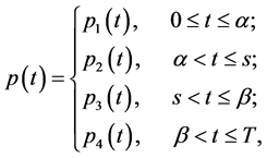
and . Consider the following BVP: find a vector-function
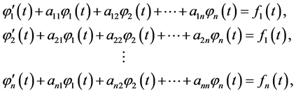
  that satisfies a system of linear first-order ordinary differential equations
 (0.1)
(0.1)
almost everywhere on an interval  and the boundary conditions
 (0.2)
(0.2)
at the points 0 and . Here
  is an
is an  matrix with the entries
  continuous on
 ;
;


 and
and 

 are
are  and
and  matrices of rank
  and
and , respectively; upper index
  denotes transposition of a matrix or a vector and the upper bar throughout the whole text of the paper that e.g. index
takes all values from 1 to ;
;  is a space of functions absolutely continuous on
  for which the derivative that exists almost everywhere on
  belongs to space
  and
and

The problem of finding a function  that satisfies on
  the equation
 (0.3)
(0.3)
and the boundary conditions
 (0.4)
(0.4)
will be called the homogeneous BVP corresponding to BVP (0.1), (0.2).
The solution  to homogeneous BVP (0.3), (0.4) is called the trivial solution.
BVP (0.1), (0.2) can be written in a scalar form:
 (0.5)
(0.5)
 (0.6)
(0.6)

Let
 (0.7)
(0.7)
be a fundamental system of solutions to (0.3) (for the definition, see e.g. [12] p. 179). Then the solutions to (0.3), (0.4) have the form

where, by virtue of (0.4), constants  must be such that
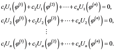 (0.8)
(0.8)
Thus, if the matrix
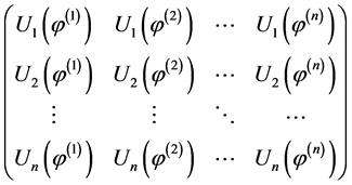 (0.9)
(0.9)
has rank , the homogeneous BVP has only the trivial solution. The inverse statement is also valid: if the homogeneous BVP has only the trivial solution then the rank of matrix (0.9) equals
  (see, for example [13] ).
Assume in what follows that homogeneous BVP (0.3), (0.4) corresponding to BVP (0.1), (0.2) has only the trivial solution or what is the same that matrix (0.9) has rank  As is known [13] , under this assumption, initial BVP (0.1), (0.2) is uniquely solvable at any right-hand sides
 , and
, and 
Formulate the notion of a BVP conjugate to (0.1), (0.2). To this end, introduce the following designations:  is the
  unit matrix;
  is the
  null matrix;

 is a square nondegenerate
  submatrix of the matrix

 ;
; 

 is an
is an  submatrix of
  obtained as a result of deleting in
  all columns of matrix
  (so that
 );
);  is an
is an  matrix such that its
  th column equals
  th column of matrix
  (its size is
 ),
),  and
and  th column equals lth column of matrix

 is an
is an  matrix such that its
  th column equals k-th column of matrix
 and
and  th column equals lth column of matrix

 is an
is an  matrix such that its
  th column equals kth column of matrix
 and
and  th column equals lth column of matrix

Introduce more similar notations: 

 is a square nondegenerate
  submatrix of the matrix


 is a
is a  submatrix of the matrix
  obtained as a result of deleting in
  all columns of matrix
  (so that
 );
);  is an
is an  matrix such that its
  th column equals kth column of matrix
  (the size of the latter is
 ),
),  and
and  th column equals lth column of matrix

 is an
is an  matrix such that its
  th column equals kth column of matrix
 and
and  th column equals lth column of matrix

 is an
is an  matrix such that its
  th column equals kth column of matrix
 and
and  th column equals lth column of matrix

By

we will denote the inner product of vectors  and
and  in the Euclidean space
Then, if  we have
 (0.10)
where the differential operator

will be called formally conjugate to operator 
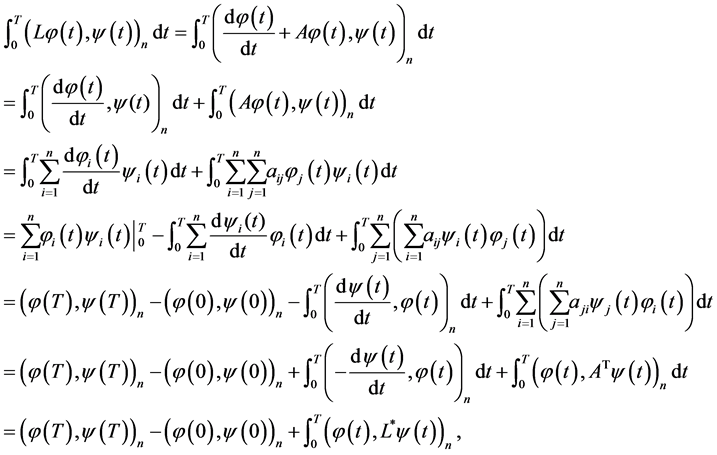
Let us show that the term  in (0.10) can be represented as
 (0.11)
Note first that

where

Then  and
and

where  and
and  are vectors composed of components of vector
  with the numbers equal to the numbers of components of vectors
  and
and , respectively. Taking into account that

we have

Analogously

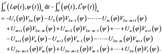
These two equalities yield representation (0.11); using the latter and (0.10), we obtain
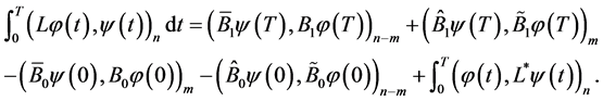 (0.12)
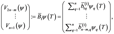
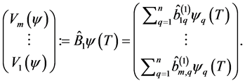
In order to write the sum of the first four terms on the right-hand side of (0.12) in a scalar form, introduce the following notations:
 (0.13)
 (0.14)
 (0.15)
 (0.16)
 (0.17)
 (0.18)
Then the Equality (0.12) can be written as
 (0.19)
Now we can introduce the notion of the adjoint BVP.
Definition 2.1 The homogeneous BVP
 (0.20)
 (0.21)
is called adjoint to homogeneous BVP (0.3), (0.4).
Definition 2.2 The inhomogeneous BVP
 (0.22)
 (0.23)
where 

 is called adjoint to inhomogeneous BVP (0.1), (0.2).
The results contained in [13] [14] imply that the following statement is valid (for more detailed explanations see [9] , pp. 9-11).
Theorem 2.1 If homogeneous BVP (0.3), (0.4) has only the trivial solution, then the corresponding adjoint BVP (0.20), (0.21) also has only the trivial solution and inhomogeneous BVP (0.22), (0.23) has one and only one solution  at any

 .
.
3. Statement of the Minimax Estimation Problem and Its Reduction to an Optimal Control Problem
Let a vector-function
 (0.24)
with the values from the space  be observed on an interval
 ; here
  is an
is an  matrix with the entries that are continuous functions on
  and
and  is an unknown random vector process whose realizations enter observations (0.24).
Denote by  the set of random vector processes
  with zero expectation
  and second moments
  integrable on
  such that their correlation matrices
  satisfy the inequality
 (0.25)
where  is a positive definite matrix of dimension
  the entries of
  and
and  are continuous on
 is a given positive number,
  denotes the trace of the matrix
 .
.
Set
 (0.26)
where 
 are given vectors;
  is a given vector-function;
 , and
, and  are positive definite matrices of dimensions
 , and
, and , respectively, the entries of
  and
and  are continuous on
 ,
,  is a given positive number.
Assume that the right-hand sides 
 and
and  of Equation (0.1) and boundary conditions (0.2) are not known exactly and it is known only that the element
  belongs to a set
  and, additionally,
  Further we also will assume, without loss of generality, that in (0.25) and (0.26)
Let a vector-function  be a solution to BVP (0.1), (0.2).
We will look for an estimation of the inner product
 (0.27)
in the class of estimates linear with respect to observations that have the form
 (0.28)
where  1 and
1 and  is a vector belonging to
 ,
,  ,
,  , and
, and  is certain constant. Then
Definition 3.1 An estimate

for which vector-function  and constant
  are determined from the condition

where

 is a solution to BVP (0.1), (0.2) at

 and
and


will be called a minimax mean square estimate of inner product  The quantity

will be called an error of the minimax estimation.
We see that the minimax mean square estimate of inner product  is an estimate at which the maximum mean square estimation error calculated for the worst realization of perturbations attains its minimum.
We will show that solution to the minimax estimation problem is reduced to the solution of a certain optimal control problem.
For every fixed  introduce vector-functions

 and
and  as a solution to the following BVP:
 (0.29)
Lemma 3.1 Determination of the minimax mean square estimate of inner product  is equivalent to the problem of optimal control of the system described by BVP (0.29) with the cost function
 (0.30)
Proof. Show first that BVP (0.29) is uniquely solvable under the condition that functions  and
and 
belong, respectively, to the spaces  and
and 
Since homogeneous BVP (0.3), (0.4) has only the trivial solution, the BVP
 (0.31)
has, in line with Theorem 2.1, the unique solution for any right-hand side, in particular, at
 (0.32)
Denote this solution by  and its restrictions on intervals

 , and
, and  by
by 

 and
and , respectively. Note that function
  is absolutely continuous on
  (see [15] ).
Let us show that the problem
 (0.33)
has one and only one solution at any vector 
Denote by 

 the coordinates of vector-function
 Let
Let 
 be the fundamental system of solutions of the equation system
  on
on  Then we can represent functions

 in the form

where  are constants. Taking into account the boundary conditions at the points
  and transmission conditions at
  in (0.33), we see that the solution to BVP (0.33) is equivalent to the solution of the following linear equation system with
  unknowns


 (0.34)
 (0.35)
 (0.36)
 (0.37)
 (0.38)
where


 denote the coordinates of vector
  and
and 

 and
and 

 denote the entries of matrices
  and
and , respectively.
Show that system (0.34)-(0.38) is uniquely solvable at any vector  To this end, note that homogeneous system (0.34)-(0.38) (at
 ) has only the trivial solution.
Indeed, setting  in Equations (0.35) and (0.36), taking into account (0.37) and the fact that

 , and
, and  because
 is the fundamental system of solutions of the equation system
  on
on  we obtain

Coefficients  satisfy Equations (0.34) and (0.38); therefore vector-function
  with the components
 is a solution to conjugate BVP (0.20), (0.21) which has only the trivial solution
  on
on  by Theorem 2.1. This implies
 , so the homogeneous linear equation system (0.34)- (0.38) (at
 ) has only the trivial solution. Consequently, system (0.34)-(0.38) and therefore BVP (0.33) which is equivalent to this system are uniquely solvable at any vector
  Then vector-functions
 form the unique solution to BVP (0.29).
Show next that the determination of the minimax estimate of inner product  is equivalent to the problem of optimal control of the system described by BVP (0.29) with the cost function (0.30).
Using the second and third equations in (0.29) and the fact that  is a solution to BVP (0.1), (0.2) at
 and
and  we easily obtain the relationships


Taking into account the equalities


and that


(we refer to the reasoning on p. 4) we obtain
Taking into notice that


and therefore


we use the last equality to obtain
 (0.39)
where

Recalling that  is a vector process with zero expectation, we use condition (0.25) and the known relationship
  that couples the dispersion
  of random variable
  with its expectation
  to obtain


which yields
 (0.40)
In order to calculate the supremum on the right-hand side of (0.40) we apply the generalized CauchyBunyakovsky inequality [16] and write this inequality in the form convenient for further analysis: for any
 , the generalized Cauchy-Bunyakovsky inequality holds
in which the equality is attained at

Setting in the generalized Cauchy-Bunyakovsky inequality


and denoting

we obtain, in line with (2.7), the inequality
where the equality is attained at

Thus,
 (0.41)
at 
Calculate the second term on the right-hand side of (0.40). Applying the generalized Cauchy-Bunyakovsky inequality, we have
 (0.42)
Here  can be placed under the integral sign according to the Fubini theorem because we assume that
  is a random process of the integrable second moment. Transform the last factor on the right-hand side of (0.42):

Taking into account that (0.25) holds, we see that (0.42) yields
 (0.43)
It is not difficult to check that here, the equality sign is attained at the element
where  is a random variable such that
  and
and  We conclude that statement of the lemma follows now from (0.40), (0.41), and (0.43).
4. Representations for Minimax Mean Square Estimates of Functionals from Solutions to Two-Point Boundary Value Problems and Estimation Errors
In this section we prove the theorem concerning general form of minimax mean square estimates. Solving optimal control problem (0.29), (0.30), we arrive at the following result.
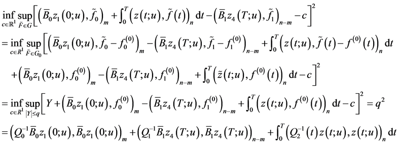
Theorem 4.1 The minimax mean square estimate of expression  has the form

where
 (0.44)

 (0.45)
and vector-functions  and
and ,
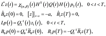
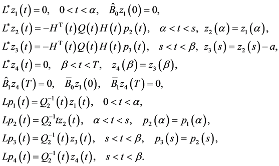
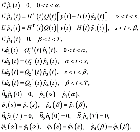
,  are determined from the solution to the problem
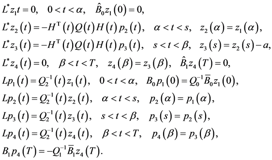 (0.46)
Here 

 and
and  The minimax estimation error
 (0.47)
Problem (0.46) is uniquely solvable.
Proof. We will solve optimal control problem (0.29), (0.30). Represent solutions 
 of problem (0.29) as
  where
where 


 and
and 


 denote the solutions to this problem at
  and
and 
 respectively. Then function (0.30) can be represented in the form

where

Since solution  of BVP (0.31) is continuous2 with respect to right-hand side
  defined by
(0.32), the function  is a linear bounded operator mapping the space
  to
to

Thus,  is a continuous quadratic form corresponding to a symmetric continuous bilinear form
 is a linear continuous functional defined on
  and
and  is a constant independent of
 . We have

Using Theorem 1.1 from [17] , we conclude that there is one and only one element  such that

Therefore

Taking into consideration the latter equality, (0.30), and designations on p. 11, we obtain
 (0.48)
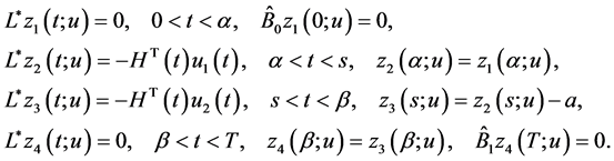
Introduce functions 

 and
and  as a unique solution to the following problem3:
 (0.49)
Now transform the sum of the last for terms on the right-hand side of (0.48) taking into notice that  and
and  We have
 (0.50)
From Equalities (0.48)-(0.50) it follows that

so that
 (0.51)
Functions 

 and
and  are absolutely continuous on segments

 , and
, and , respectively, as solutions to BVP (0.49); therefore, functions
  and
and  that perform optimal control are continuous on
  and
and  Replacing in (0.29) functions
  and
and  by
by  and
and  defined by formulas (0.51) and denoting
 we arrive at problem
(0.46) and equalities (0.44).
Taking into consideration the way this problem was formulated we can state that its unique solvability follows from the fact that functional (0.30) has one minimum point .
.
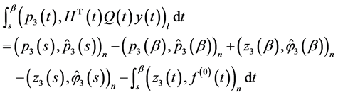
Now let us prove representation (0.47). Substituting into formula  expressions (0.44) for
and  we have
 (0.52)
Next, we can apply the reasoning similar to that on p. 4 and use (0.46) to obtain

which yields
 (0.53)
In a similar manner, using the equality

we obtain
 (0.54)
Relationships (0.52)-(0.54) yield

which is to be proved.
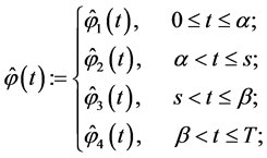
It is easy to see that function  defined by (0.45) and the function
 (0.55)
satisfy the following uniquely solvable BVP
 (0.56)
where


and  is the characteristic function of interval
 .
.
Now Theorem 4.1 can be restated as follows:
Theorem 4.1' The minimax estimate of expression  has the form

where
 (0.57)

and vector-functions  and
and  are determined from the solution to problem 0.56.
Obtain now another representation for the minimax mean square estimate of quantity  which is independent of
  and
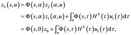
and . To this end, introduce vector-functions

 and
and  as solutions to the problem
 (0.58)
at realizations  that belong with probability 1 to space
Note that unique solvability of problem (0.58) at every realization can be proved similarly to the case of (0.46). Namely, one can show that solutions to the problem of optimal control of the system


with the cost function

can be reduced to the solution of problem (0.58) where the optimal control  is expressed in terms of the solution to this problem as
 ; the unique solvability of the problem follows from the existence of the unique minimum point
  of functional
 .
.
Considering system (0.58) at realizations  it is easy to see that its solution is continuous with respect to the right-hand side. This property enables us to conclude, using the general theory of linear continuous transformations of random processes, that the functions

 considered as random fields have finite second moments.
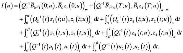
Theorem 4.2 The following representation is valid

Proof. By virtue of (0.44) and (0.58),
 (0.59)
Next,
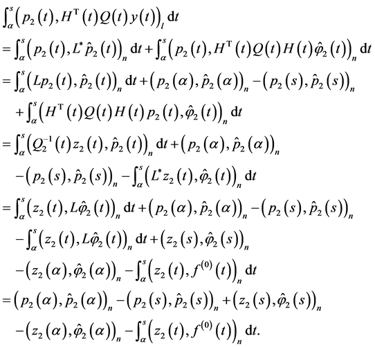 (0.60)
Similarly,
 (0.61)
From (0.59), (0.60), and (0.61) it follows
 (0.62)
However,
 (0.63)
 (0.64)
Subtracting from (0.63) equality (0.64), we obtain

or
 (0.65)
Since


we can use the latter equalities, (0.65), and the fact that  is a symmetric matrix to obtain
 (0.66)
Performing a similar analysis, one can prove that
 (0.67)
From (0.66), (0.67), and (0.62) and the expression for  it follows

The theorem is proved.
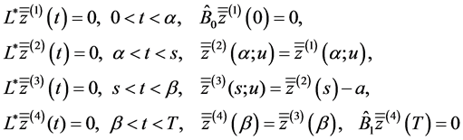
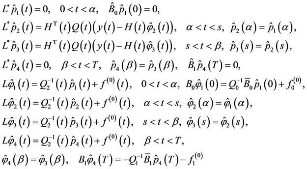
As is easily seen from (0.58), the functions  and
and  defined by
and

satisfy the following uniquely solvable BVP:
 (0.68)
at realizations  that belong with probability 1 to space
 .
.
Thus, Theorem 4.2 can be restated in the following form.
Theorem 4.2' The minimax mean square estimate of expression  has the form

where vector-function  is determined from the solution to problem (0.68).
Remark. Function  can be taken as a good, in certain sense, estimate of solution
  of initial BVP (0.1), (0.2) on
As an example, consider the case when a vector-function  is observed on an interval
 , where a vector-function
  with values in
  is a solution to the BVP
 (0.69)
and operator  is defined by the relation

where  is a positive definite
  -matrix whose entries are continuous functions on
Note that this problem has the unique classical solution if  is continuous on
  and the unique generalized solution if
Assume that, as well as in the previous case,  is an
is an  matrix with the entries that are continuous functions on
  and
and  is a random vector process with zero expectation
  and unknown
  correlation matrix
 . Assume also that domains
  and
and  are given in the form (0.25) and (0.26) where matrices
 , and
, and  entering (0.26) have dimensions

 , and
, and 
Write Equation (0.69) as a first-order system by setting 
 and introducing a vector-function


with  components, a vector
  with
with  components, a
  -matrix

matrices  and
and . Then system (0.69) can be written as
 (0.70)
 (0.71)
Applying Theorems 1 and 2 and performing necessary transformations in the resulting equations that are similar to (0.46) and (0.58) (in terms of the designations introduced above) we prove the following Theorem 4.3 The minimax mean square estimate of expression  has the form

where


 and vector-functions
 ,
,  and
and  are determined from the solutions to the problems


and


respectively.
5. Minimax Mean Square Estimates of Solutions Subject to Incomplete Restrictions on Unknown Parameters
Assume again that observations have form (0.24) and unknown parameters ,
,  , and
, and  belong to the domain
 (0.72)
where  is given in (0.26). The correlation function of process
  belongs to domain (0.25). Introduce the set
 (0.73)
here  where
where  is the solution to BVP (0.29).
Lemma 5.1

where
 (0.74)
This lemma can be proved using formula (0.39).
Lemma 5.2  is a convex closed set in the space
 .
.
Proof. The convexity of set  is obvious. Let us prove that this set is closed.
Note that functions  and
and  can be represented as
 (0.75)
where  and
and  are known matrix functions with the elements from
  and
and  and
and  are vectors. Expression (0.75) can be obtained if we introduce a vector
  such that
  Then
Then 
where  is a solution to the equation

and  is the unit matrix. Next,

Since BVP (0.29) is uniquely solvable, there exists one and only one vector  satisfying the system of algebraic equations

Solving this system we determine  in the form

where  is a known matrix function continuous on
  and
and  is a known vector. Taking into account this equality, we obtain expressions (0.75). From these relationships, it follows that if a sequence
  converges in
  to a function
  then
then


which proves that  is a closed set.
Assume now that  is nonempty. Then the following statement is valid.
Theorem 5.1 There exists the unique minimax mean square estimate of expression  which can be represented in the form (0.44) at
  where vector-functions
  and
and  solve the equations
 (0.76)
Proof. Similarly to Theorem 4.1 one can show that for  the following equality holds

where

and  are solutions to Equations (0.29) at
  and
and 
 is a strictly convex lower semicontinuous functional on a closed convex set
  and
and  Therefore there exists one and only one vector
  such that
  This vector can be determined from the relationship

where


 and
and  are Lagrange multipliers.
Further analysis is similar to the proof of Theorem 4.1. Let vector-functions  and
and ,
,  be solutions to the system
 (0.77)
Theorem 5.2 Assume that for any vector  set
set  is nonempty. Then system (0.77) is uniquely solvable and the equality

holds Proof. Introduce functions ,
,  as a solution to the BVP


where  Define a set

Since  is nonempty, the same is valid for
  for any vector
 . Similarly to the case of
  one can show that
  is a convex closed set. Denote by
  the functional of the form

One can show, following Theorem 5.1, that on set  there is one and only one point of minimum of functional
  namely,

where functions  and
and  are determined from system (0.77). The proof of the equality

is similar to that in Theorem 4.2.
6. Conclusions
For a system described by a one-dimensional two-point BVP with decoupling boundary conditions at the endpoints of the interval and quadratic restrictions imposed on the unknown deterministic data and the second moments of observation noise, we have obtained guaranteed mean square estimates of inner product  where
where  is the unknown solution of the BVP at a point
  and
and . Guaranteed estimates are obtained using the duality of the problems of estimation and optimal control. We have shown that guaranteed mean square estimates and estimation errors are expressed via solutions to special optimal control problems for conjugate BVPs. The solutions to these optimal control problems enable one to find explicit expressions for estimates and estimation errors both for distributed and point observations.
The obtained results are applied to minimax estimation of solutions of two-point BVPs for linear ordinary second-order differential equations.
Methods and results of the paper may be used for estimation under uncertainties of the states of the systems described by more general linear BVPs for different classes of functional--differential equations; in particular, for systems of differential equations with impulse perturbations, differential equations with multipoint conditions, and in several other cases.
7. Results of Numerical Experiments
Let realizations of the random variables
 (0.78)
be observed. Here  are independent random variables for which
 ;
;  is a solution of the BVP
 (0.79)
 (0.80)
and

are eigenfunctions of the operator , where
  .
.
We assume that function  is not known exactly and is chosen arbitrarily from the set
 , where
  is a certain constant.
Applying the technique similar to the estimation methods developed in Section 4, it is possible to obtain expressions for the minimax mean square estimates in the case when observations have the form (0.78). In particular, in this case the function  which approximates the solution
  of BVP (0.79)-(0.80) on the interval
  is determined from the system


and can be represented in the form

The exact solution  and its estimate
  (bold curves) calculated on the basis of the modelled observations are presented in Figure 1 and Figure 2. Calculations are performed at
 ,
,  , and
, and  for
for 
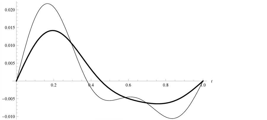
Figure 1. Exact solution  and its estimate
  (bold curve) calculated at q = 1, w = 1, N = 5,
 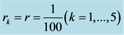 , and
, and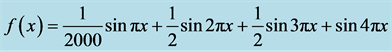 .
.
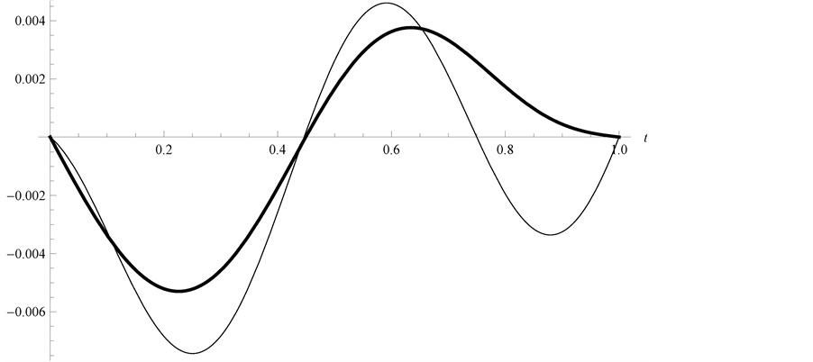
Figure 2. Exact solution  and its estimate
  (bold curve) calculated at q = 1, w = 1, N = 5,
  , and
, and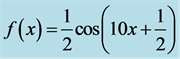 .
.
using the parameters  and
and  (Figure 1) and
  and
and  (Figure 2).
As can be seen from these figures, parameter  plays the crucial role as far as the estimation quality is concerned. In fact, this parameter directly influences the signal-to-noise ratio.
The calculations were performed using Wolfram Mathematica.
References
- Kalman, R. (1960) A New Approach to Liner Filtering and Prediction Problems. Journal of Basic Engineering, 82, 35-45.
- Kalman, R. and Bucy, R. (1961) New Results in Liner Filtering and Prediction Theory. Transactions of the ASME-Journal of Basic Engineering, 83, 95-108. http://dx.doi.org/10.1115/1.3658902
- Krasovskii, N. (1968) Theory of Motion Control. Nauka, Moscow.
- Kurzhanskii, A. (1977) Control and Observation under Uncertainties. Nauka, Moscow.
- Kirichenko, N. and Nakonechnyi, O. (1977) A Minimax Approach to Recurrent Estimation of the States of Linear Dynamical Systems. Kibernetika, 4, 52-55.
- Nakonechnyi, O. (1979) Minimax Estimates in Systems with Distributed Parameters. Preprint 79, Acad. Sci. USSR, Inst. Cybernetics, Kyiv, 55 p.
- Kuntsevich, V. (2005) Accuracy of Construction of Approximating Models under Bounded Measurement Noises. Automation and Remote Control, 66, 791-798. http://dx.doi.org/10.1007/s10513-005-0123-0
- Kurzhanski, A. and Valyi, I. (1997) Ellipsoidal Calculus for Estimation and Control. Birkhauser Verlag, Basel. http://dx.doi.org/10.1007/978-1-4612-0277-6
- Nakonechnyi, O., Podlipenko, Y. and Shestopalov, Y. (2009) Estimation of Parameters of Boundary Value Problems for Linear Ordinary Differential Equations with Uncertain Data. arXiv:0912.2872v1, 1-72.
- Podlipenko, Y. (2005) Minimax Estimation of Right-Hand Sides of Noetherian Equations in a Hilbert Space under Uncertainty Conditions. Reports of the National Academy of Sciences of Ukraine, 12, 36-44.
- Basar, T. and Bernhard, P. (1991) H-Optimal Control and Related Minimax Design Problems. Birkhäuser, Basel.
- Fedoryuk, M. (1985) Ordinary Differential Equations. Nauka, Moscow.
- Naimark, M. (1969) Linear Differential Operators. Nauka, Moscow.
- Krein, S. (1971) Linear Equations in the Banach Space. Nauka, Moscow.
- Atkinson, F. (1964) Discrete and Coninuous Boundary Value Problems. Academic Press, New York.
- Hutson, V., Pym, J. and Cloud, M. (2005) Applications of Functional Analysis and Operator Theory. Vol. 200, 2nd Edition, Mathematics in Science and Engineering, Elsevier Science, Amsterdam.
NOTES

*Corresponding author.

1If  then the minimax estimation problem can be solved in a similar manner but somewhat simpler.

2This continuous dependence follows from the representation of function  in terms of Green's matrix
  of BVP (0.31) (see , p. 115):


3The unique solvability of problem (0.49) can be proved similarly to problem (0.29).