Advances in Pure Mathematics
Vol.3 No.9(2013), Article ID:40886,10 pages DOI:10.4236/apm.2013.39097
Global Properties of Evolutional Lotka-Volterra System
1Department of Mathematics, Graduate School of Science, Hiroshima University, Higashi-Hiroshima, Japan
2Research Center for Environmental Risk, National Institute for Environmental Studies, Tsukuba, Japan
Email: yoshinom@hiroshima-u.ac.jp, ytanaka@nies.go.jp
Copyright © 2013 Masafumi Yoshino, Yoshinari Tanaka. This is an open access article distributed under the Creative Commons Attribution License, which permits unrestricted use, distribution, and reproduction in any medium, provided the original work is properly cited. In accordance of the Creative Commons Attribution License all Copyrights © 2013 are reserved for SCIRP and the owner of the intellectual property Masafumi Yoshino, Yoshinari Tanaka. All Copyright © 2013 are guarded by law and by SCIRP as a guardian.
Received November 9, 2013; revised December 9, 2013; accepted December 15, 2013
Keywords: Lotka-Volterra System; Global Dynamics; Evolution
ABSTRACT
We will study global properties of evolutional Lotka-Volterra system. We assume that the predatory efficiency is a function of a character of species whose evolution obeys a quantitative genetic model. We will show that the structure of a solution is rather different from that of a non-evolutional system. We will analytically show new ecological features of the dynamics.
1. Introduction
In this paper, we study global behavior of an evolutional Lotka-Volterra system for three species
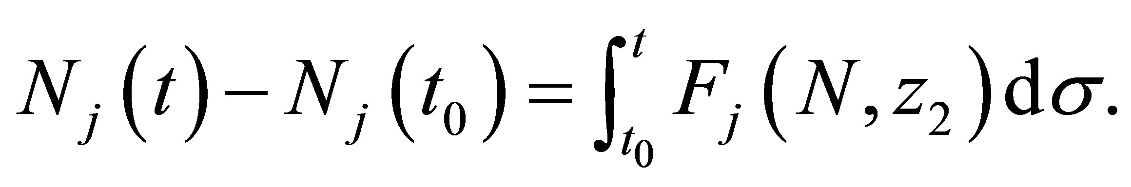
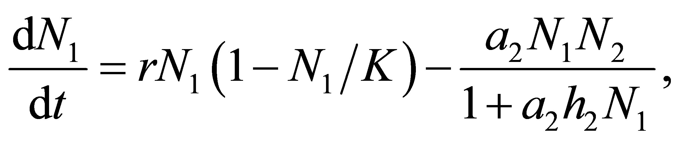 (1.1)
(1.1)
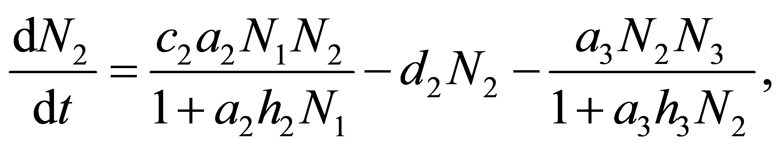 (1.2)
(1.2)
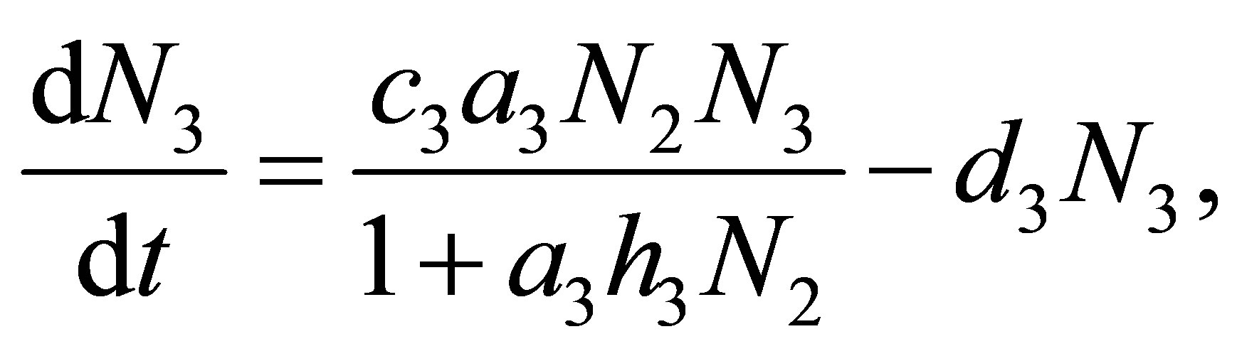 (1.3)
(1.3)
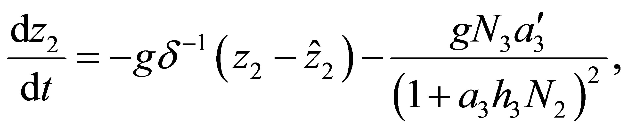 (1.4)
(1.4)
for the unknown quantities  and
and  which are the population of jth species and the mean character value of the second species, respectively. Here
  are certain constants, and
  and
and  are death rate of the second and the third species, respectively. The quantities
  and
and  are the predatory efficiency of the second and the third species, respectively. The number
  is the mean character value of the second species with minimal cost. The quantity
  is the additive genetic variance and
  is the cost of evolution, namely, if
  decreases, then the cost increases.
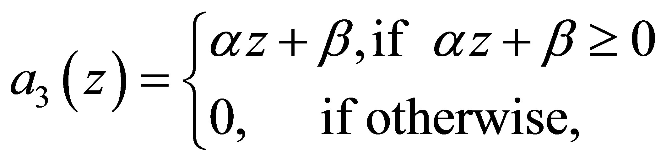
The effect of evolution is expressed in terms of (1.4) and the condition that the predatory efficiency  is given by
 (1.5)
(1.5)
where  is a given constant and
  is a function of
 . An example of a3 is given by (C.1) in Section 3. Equation (1.4) follows the quantitative genetical model (cf. [1-5]. See also Section 7). The evolutional Lotka-Volterra system for two species was studied in [3], where rather detailed numerical analysis was made. As for the system for three species, very little is known as to global behavior of solutions even from a numerical point of view. In this paper, we shall make the analytical study of evolutional Lotka-Volterra model for three species and show several new phenomena caused by evolution.We also refer [6] as to non-evolutional case.
Let  Let
Let  and
and  and
and  be given. We first prove that (1.1)-(1.4) with the initial condition
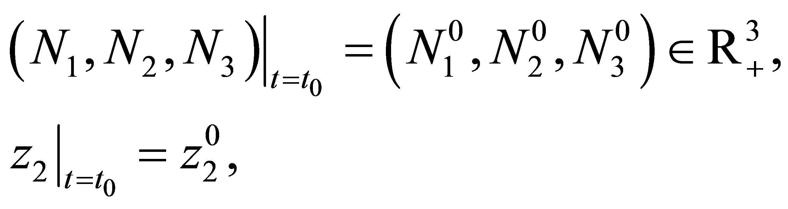 (1.6)
(1.6)
have unique smooth time global solution. (cf. Theorem 2). Then, in terms of estimate of a solution obtained in the proof of Theorem 2, we study behaviors of a solution related to evolution. Indeed, we will show that the behavior of a solution near the equilibrium point is different from those in the case of tea-cup attractors for a nonevolutional system. Namely, the decay of the predator  starts before the quantity
  becomes small because the predatory efficiency a3 tends to zero, by evolution. We remark that although
  plays an important role in the non-evolutional system near equilibrium point, the quantity
  is crucial in the evolutional one. This is because the quantity
  is related with the dynamics of evolution. We remark that the effect of evolution in our system is intermittent in the sense that in some subdomain of the phase space flactuations of pray
  occur as in the case of non-evolutional model, while in other subdomain, evolution stabilizes large fluctuations of
  and
and . We also discuss the role of γ in (C.1), which is related with the sensitivity of evolution to the character bias
 . (cf. Lemma 3 and Section 4 for the case of a linear efficiency). In Section 5, we study the uniform convergence of solutions of an evolutional system as the cost of evolution tends to infinity, i.e.,
  decreases to zero.
2. Time Global Solution
We shall study the global existence and uniqueness of a solution of the initial value problem. We assume that  is the twice continuously differentiable function which satisfies
 (2.1)
(2.1)
for some . Moreover we suppose that there exist
  and
and  such that
 (2.2)
(2.2)
The following local existence and uniqueness theorem is well known.
THEOREM 2.1. Assume (2.1) and (2.2). Then there exists a  such that the system of Equations (1.1)- (1.4) with the initial conditions (1.6) has a unique continuously differentiable solution
 ,
,  in
in 
In the following we study the existence of a global solution. We require the condition
 (2.3)
(2.3)
Remark. If  for some j, then, by the uniqueness, any solution of (1.1)-(1.4) satisfies
 . Hence it reduces to a system with less unknown quantities. Note that we avoid this case in (2.3).
We have
THEOREM 2.2. Suppose that (2.3) is satisfied. Then the system of Equations (1.1)-(1.4) with the initial condition (1.6) has a unique global solution in 
Proof. First we will show the apriori estimate  for all
 . Suppose that this is not true. Then, by the continuity of
  and
and  in (2.3) we can take the smallest time
  such that
  Assume that
  If we set
  in (1.1)-(1.4), then we have
 (2.4)
(2.4)
By the local existence and uniqueness theorem, Equations (2.4) with the initial condition  has a unique solution. We denote the solution by
 . Then (1.1)-(1.4) with the initial value
  at
at  has a solution
  By the uniqueness of the solution we obtain
 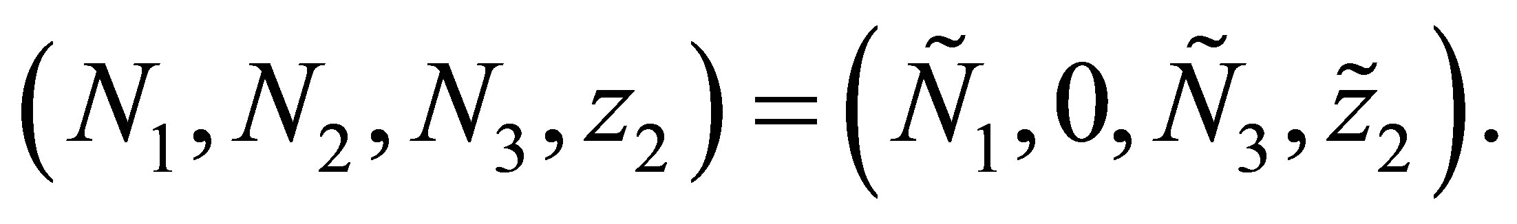 It follows that
 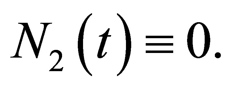 Because
  by (2.3), we have a contradiction. Hence we have
  By the continuity of
  one may assume that
  in a sufficiently small neighborhood of
 . Then, the second term in the right hand side of (1.1) satisfies
  in a sufficiently small neighborhood of
  On the other hand, since
 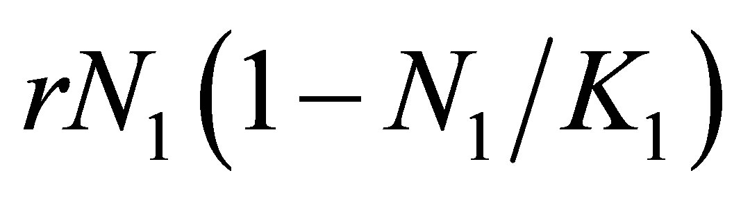 can be made arbitrarily small by taking a neighborhood of small, it follows that
  there. Hence
  is a decreasing function. This contradicts to
 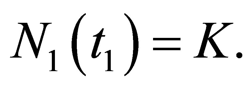 Therefore, there is not
  such that
  which shows the desired estimate.
Next we will estimate N2 from the above. Take  that
that  and add ε times (1.2) to (1.1). Then we have
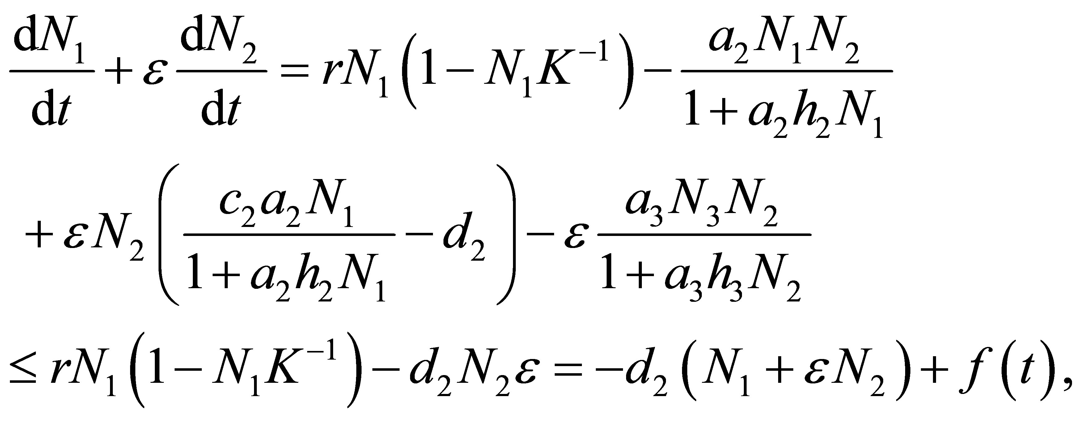 (2.5)
(2.5)
where 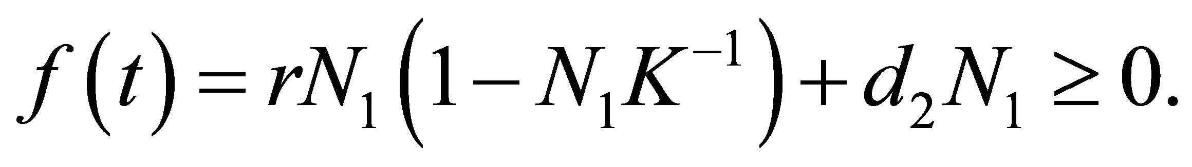
Hence, by setting 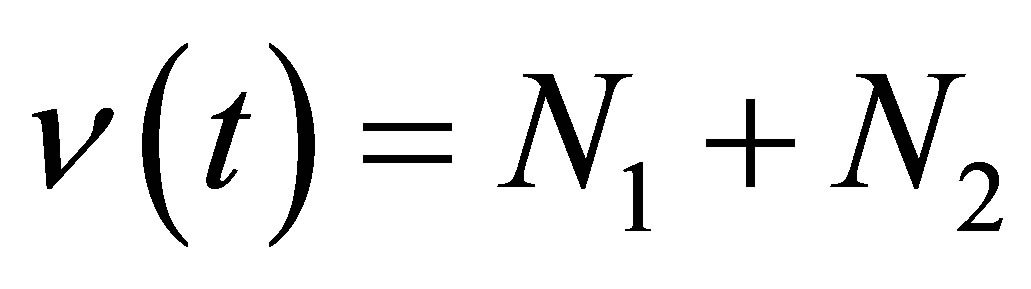 we obtain
 (2.6)
(2.6)
Multiplying  to both sides, and integrating from
  to
to  we obtain
 (2.7)
(2.7)
By the apriori estimate there exists M > 0 depending only on r, K and 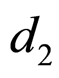 such that
 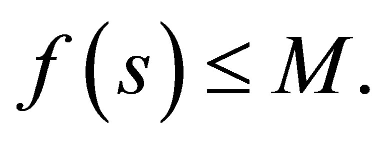 Hence we have

Because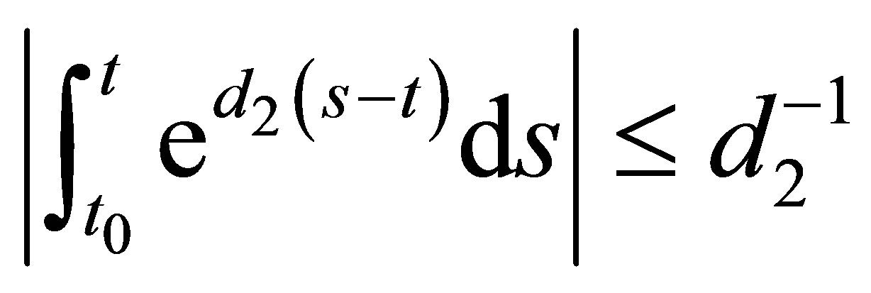 , we obtain
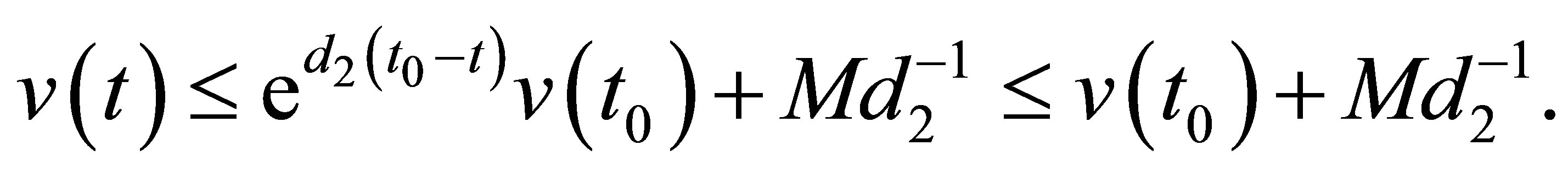 (2.8)
(2.8)
It follows that, for 
 (2.9)
(2.9)
Note that the right hand side quantity depends on the initial value and the equation and depends neither on δ > 0 nor on g > 0.
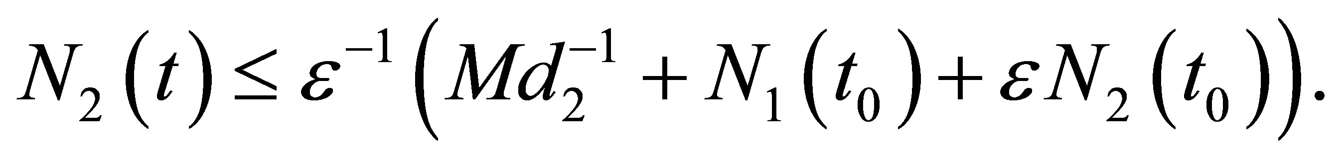
We make the same argument for  Take ε so that
  and add ε times (1.3) to (1.2). Then we have
 (2.10)
where

By setting 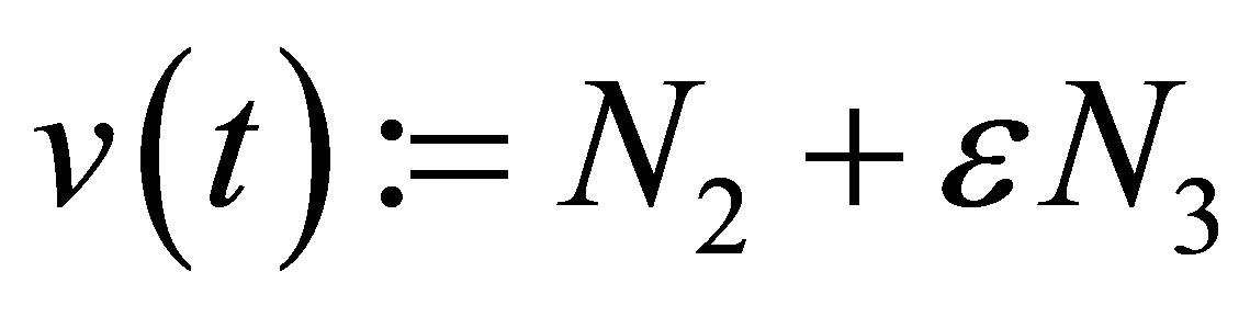 we obtain the equation
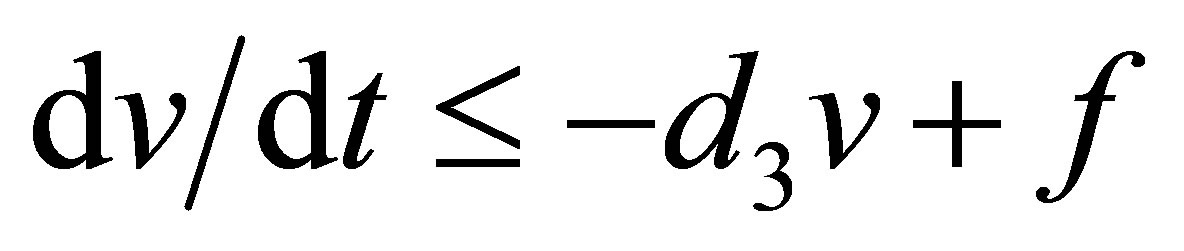 . Because this equation has a similar form as in the case
 , we can choose a constant
  depending only on
  and the initial values so that
  Then we argue in the same way and we obtain
 (2.11)
In view of the definition of v we have
 (2.12)
Next we will estimate  from the below. By the estimates of
  and
and  from the above there exists
  such that
  It follows that

By integrating from  to t we obtain
 (2.13)
We will estimate N2 from the below. There exist constants  depending on the equation and the initial values such that,
  Hence we have
By integrating the inequality from  to t we obtain
 (2.14)
The estimate of  from the below can be shown by simple computations.
 (2.15)
Next we will prove
 (2.16)
Indeed, we have (2.16) for  by the initial condition. It follows that if
  is sufficiently small, then (2.16) holds true.
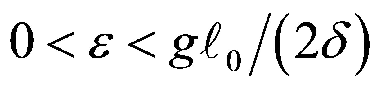
In order to prove (2.16) we assume that there exists  such that either
  or
or  holds and we show the contradiction. For the sake of simplicity let us assume the former case holds. The latter case can be treated in the same way.By the estimate of
  from the above we have, for any
 ,
,  there exists a neighborhood V of
  such that if
  then
then 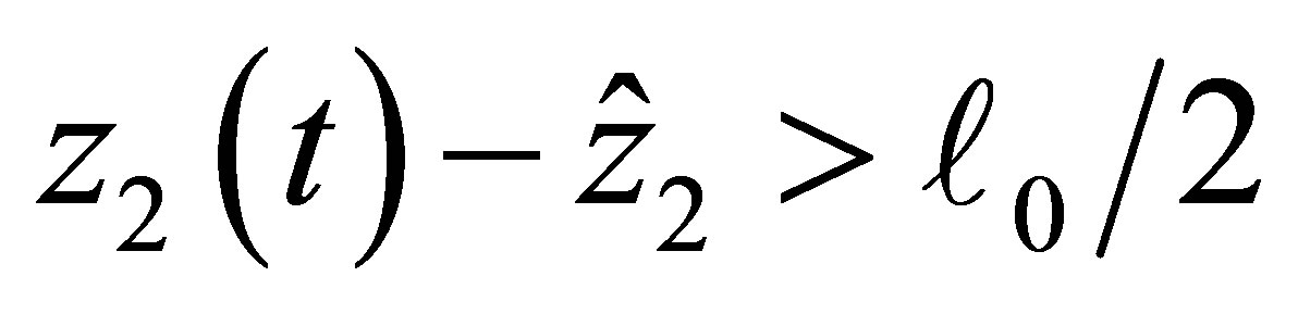 and
and  hold. Hence we have
 (2.17)
If 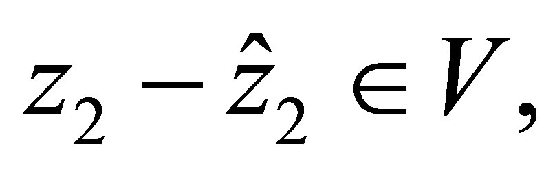 then the right hand side of (2.17) is negative. Therefore
  is decreasing near
 . This implies that
  does not tend to
  when
when . Because
  is continuous, we have
 . This is a contradiction. Hence we have the desired estimate.
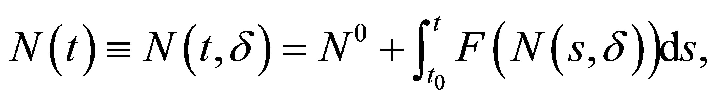
We shall prove the existence of a global solution. Set  and let
  be the maximal interval for which
  and
and  are defined. If
 , then we are done. Assume that
  We will show that the limits
  and
and  exist. We set
  where
where  is the right hand sides of the Equations (1.1)-(1.4), respectively. We write (1.1)-(1.4) into an equivalent system of integral equations
 (2.18)
By the apriori estimates from the above,  is bounded on
 . Hence there exists M such that
  It follows that the limit
  exists. If we define
 , then
  is continuous up to
 . We will show that it is
 . For this purpose it is sufficient to show that
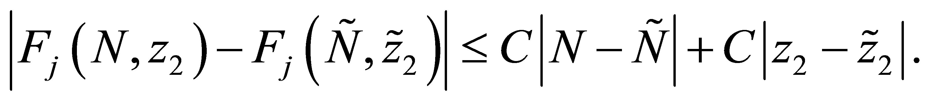
  We note that
  is Lipschitz continuous in each variable because we have apriori estimates of N and
 . Namely there exists C > 0 independent of N and
  such that
Hence, by (1.1)-(1.4) we have

This proves the assertion. We can similarly prove for  .We can solve (1.1)-(1.4) with the initial values
  and
and  at
at . Then by the unique existence of the solution we can extend
  and
and  to some neighborhood of
 . This contradicts to the definition of
 . Hence we have
 . This ends the proof.
Remark. 1) We remark that the apriori estimate of a solution does not depend on the cost of evolution  and the additive genetic variance g>0. This means that the evolution of a character has little effect to the bound of sum of populations of three species.
2) As a corollary to Theorem 2 we see that if there is no effect of evolution, i.e.,  then (1.1)- (1.3) with the initial condition (1.6) has a unique global solution. Indeed, (1.1)-(1.4) can be split into (1.1)-(1.4),
  The latter equation can be integrated. In view of the uniqueness of the solution of (1.1)-(1.4) we see that (1.1)-(1.3) has a unique solution.
3. Intermittency of Evolution Effect
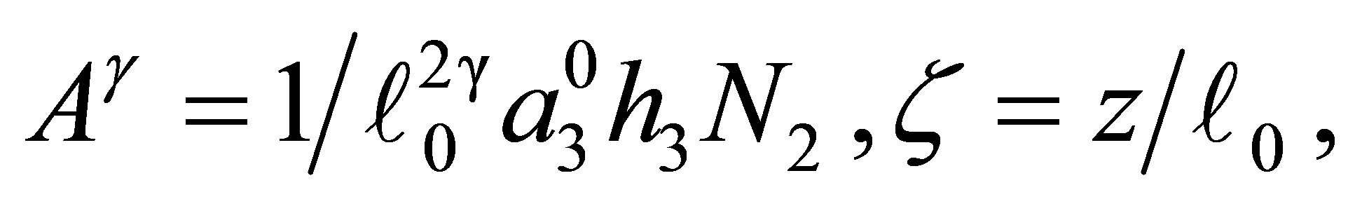
We shall study the effect of evolution to dynamics of (1.1)-(1.4).More precisely, we will study how the dynamics of (1.4) is related with that of (1.1)-(1.3).By setting  we write (1.4) in the form
 (3.1)
(3.1)
Let  be an integer and
  and
and  be constants. We assume
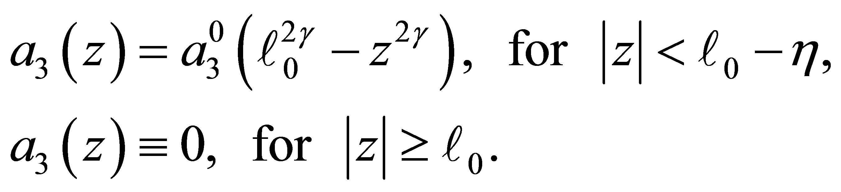 (C.1)
(C.1)
We also assume that  is twice continuously differentiable and nonnegative in the closed intervals
  and
and . If we denote the right-hand side of (3.1) by
 , then, by (C.1) we have
 (3.2)
(3.2)
on 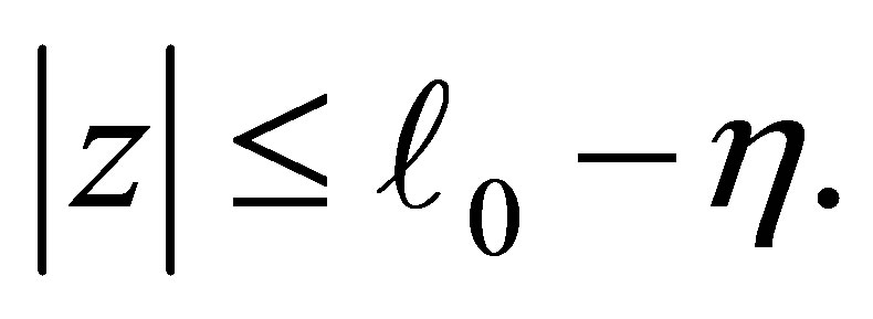 We define
 on
on 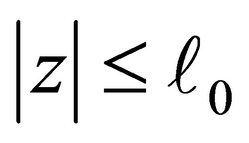 by the right-hand side of (3.2). Define, for
 (3.3)
(3.3)
We first study the behavior of .
.
LEMMA 3.1. 1) Assume  Suppose that
 . Then
  has a unique zero z = 0 in the interval
  and
and  is negative on
 .
.
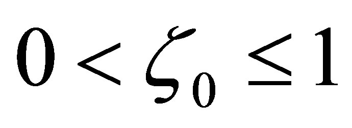
Assume . Then
  has simple zeros,
  and 0 on
 . The function
  is negative on the intervals
  and
and , while it is positive on
  and
and . (cf. Figure 1).
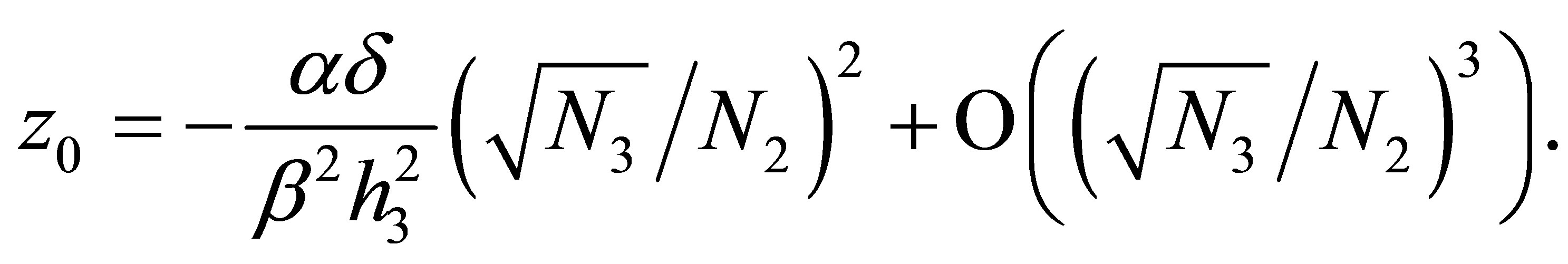
Moreover, there exists  such that z0 has an asymptotic behavior
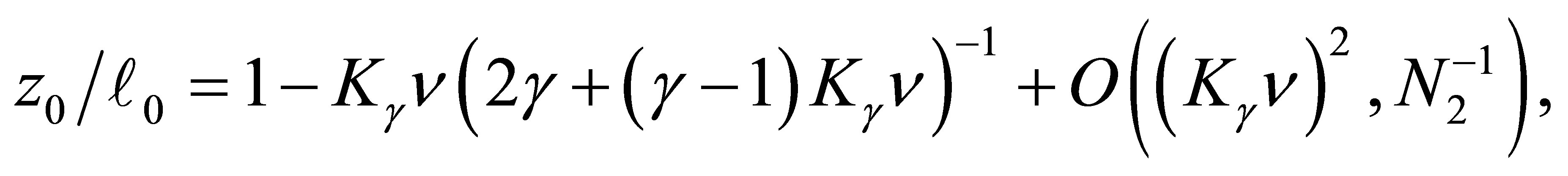 (3.4)
(3.4)
when 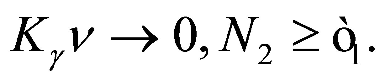 Similarly we have
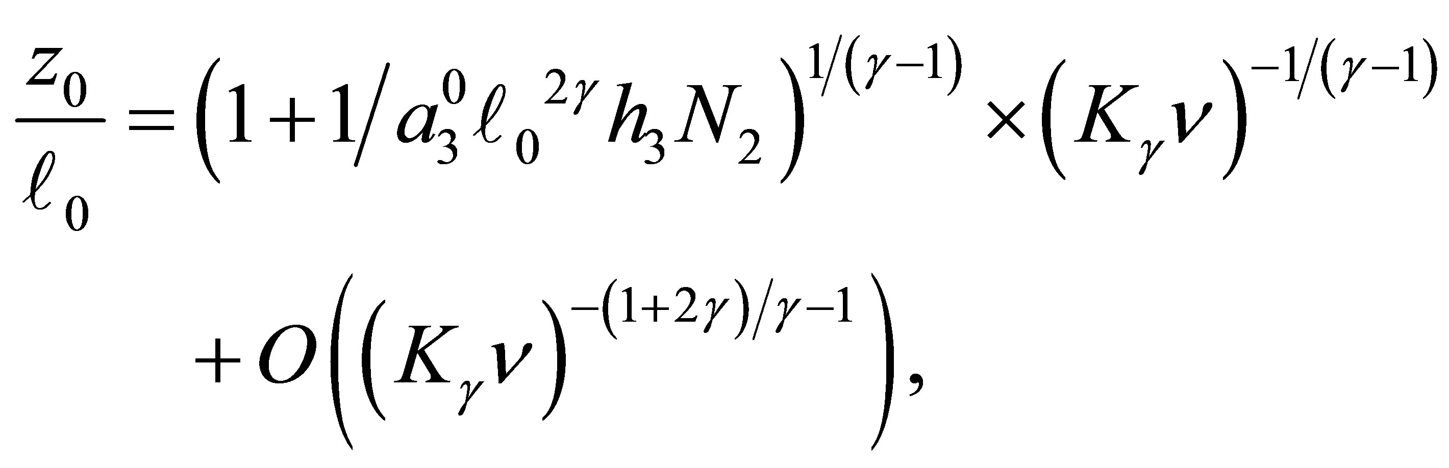 (3.5)
(3.5)
when 
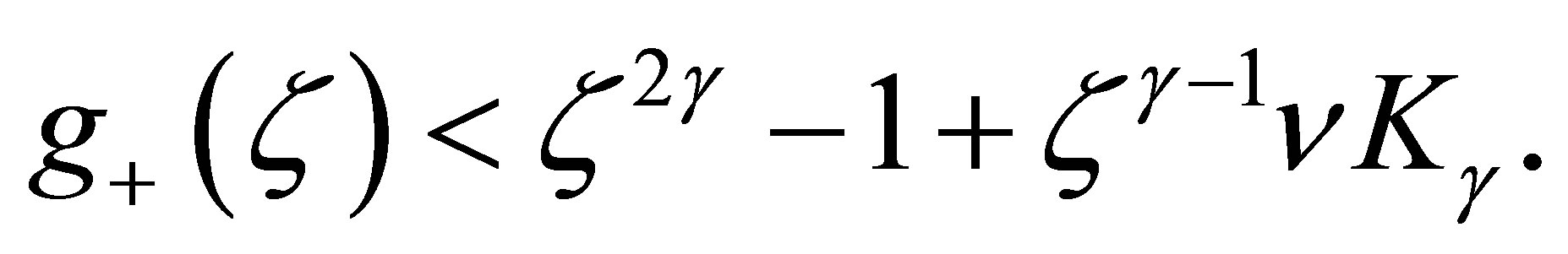
2) Assume  If
If  then
then  has simple zeros,
  and 0 on
 .
.
The function  is negative on the intervals
 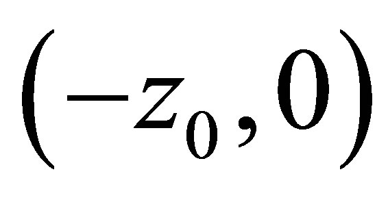 and
and 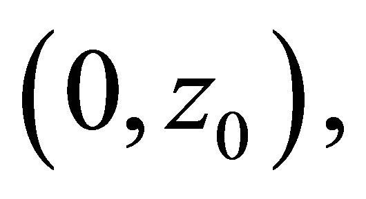 while it is positive on
 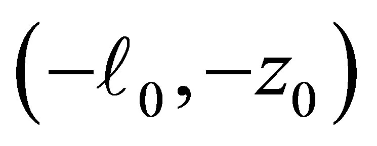 and
and . (cf. Figure 1).
If  then
then  has a unique zero z = 0 in
  and
and  is positive on
  (cf. Figure 2).

Figure 1. .
.
Proof. We divide the proof into 5 steps.
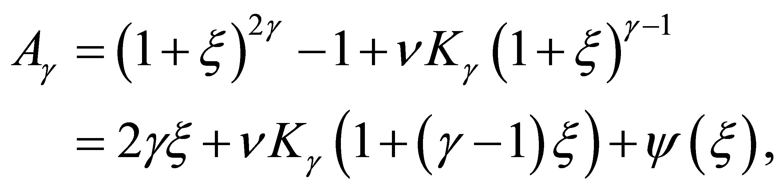
Step 1. By (C.1) we have
 (3.6)
(3.6)
Set
 (3.7)
(3.7)
and define
 (3.8)
(3.8)
We consider the zeros and the sign of  in the interval
Step 2. First we consider the case  Assume that
  is an odd integer. Because
  is an even integer, we have
 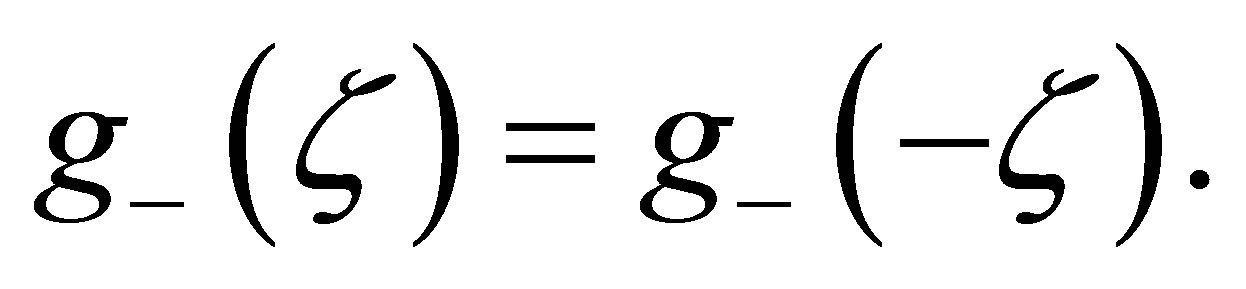 We have
  and
and . Because we easily see that
  if
if , it follows that
  has no zero point on
 .
.
In order to study the zero of  in (0,1), note
 . One easily see that the assumption
  is equivalent to
  Because
  on (0,1], we see that
  has only one zero point in the interval (0,1] if
  In view of (3.6) we conclude that
 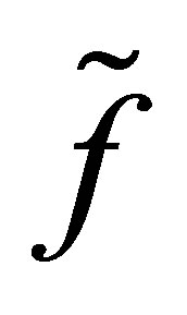 has zero points
  and 0 in the interval
  for some
 . It is also clear that if the opposite inequality
  holds, then
 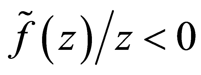 on
on .
.
Next we consider the case  is even. By the same way as in the odd case, we have
 ,
,  and
and 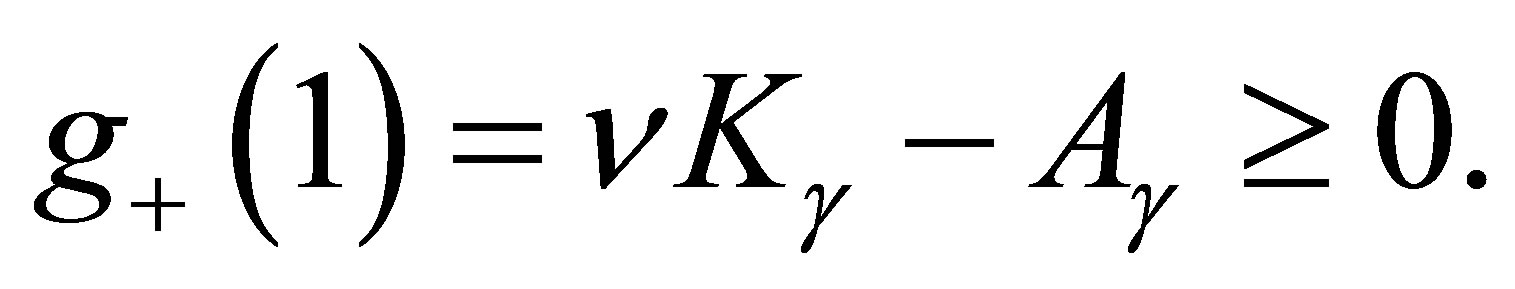 Since
Since  is strictly increasing on (0,1), there exists unique
 ,
,  such that
 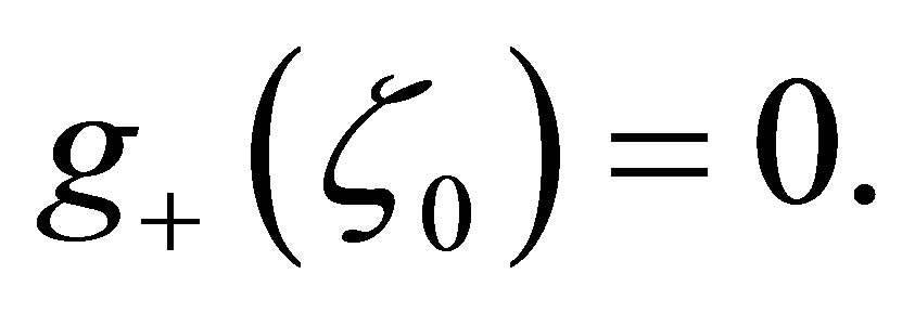 In order to show that
  has no zero on
 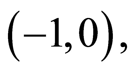 we note
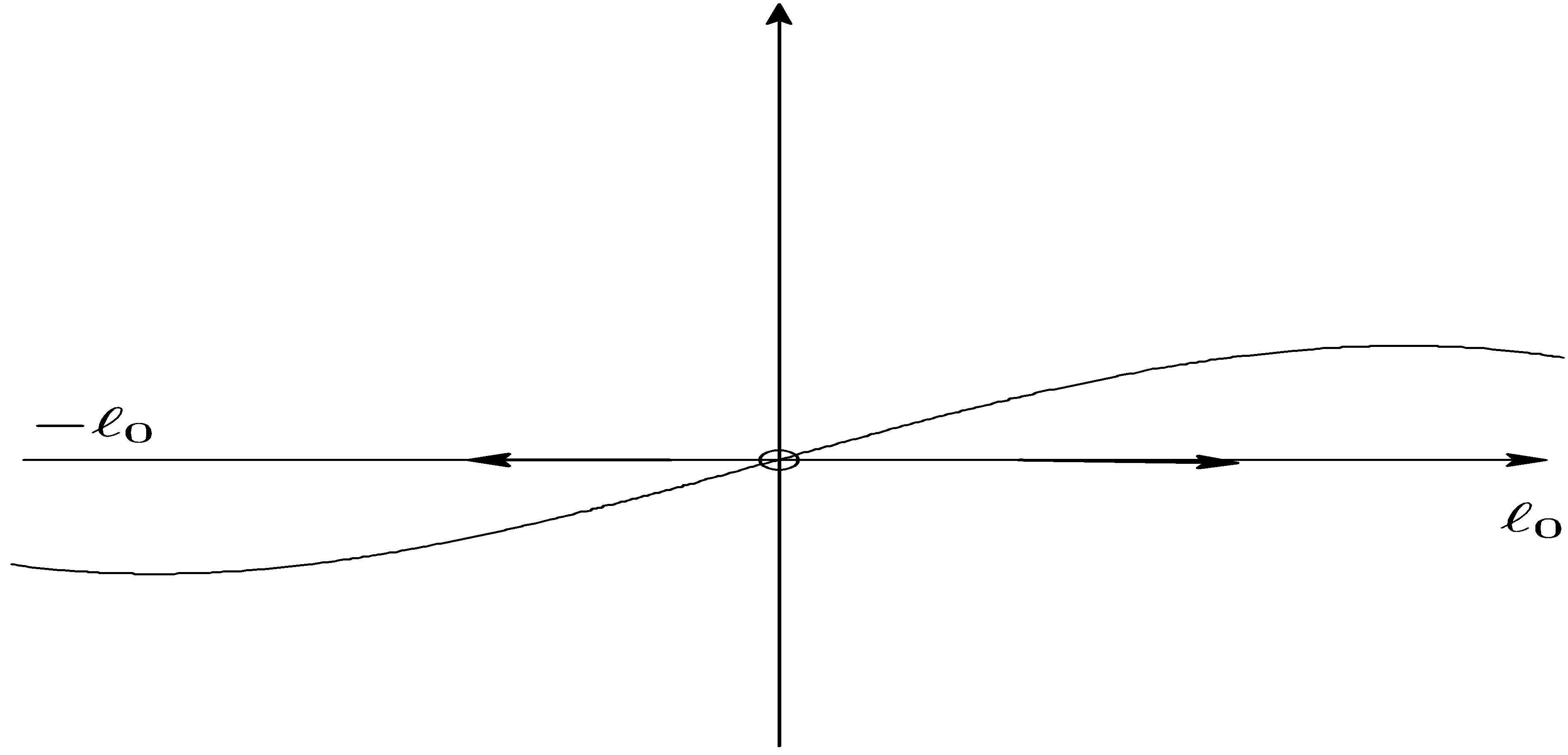
Figure 2.  and
and 
 Because
 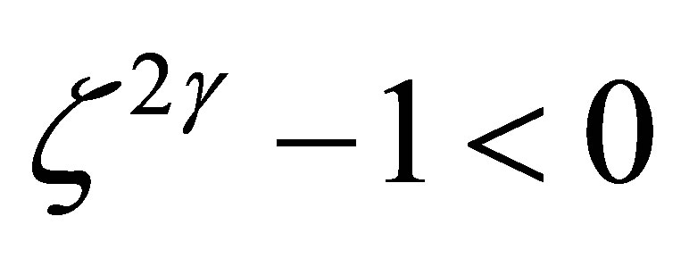 and
and
 on
on , we see that
  has a unique zero point
  on
on . Clearly,
  has only one zero
 , because
  for all
  which proves the assertion. The sign of
  is almost clear from the definitions of
  and the argument in the above.
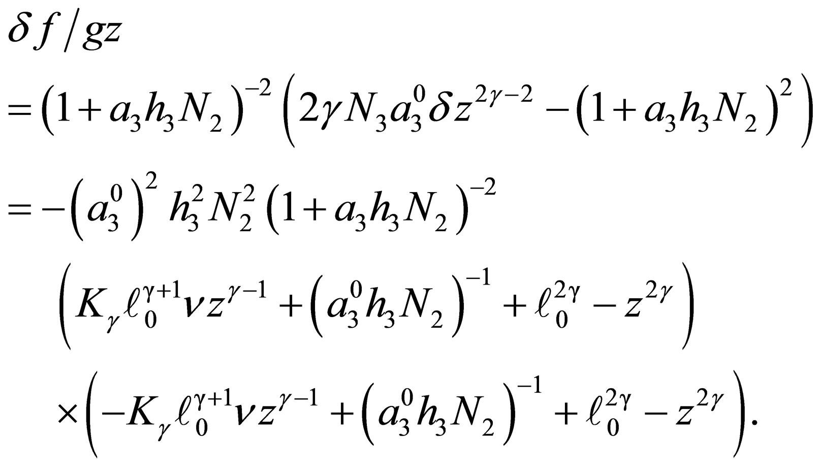
Step 3. We will show the asymptotic formula of  in (3.4). In view of the argument in Step 2 we may consider
If we set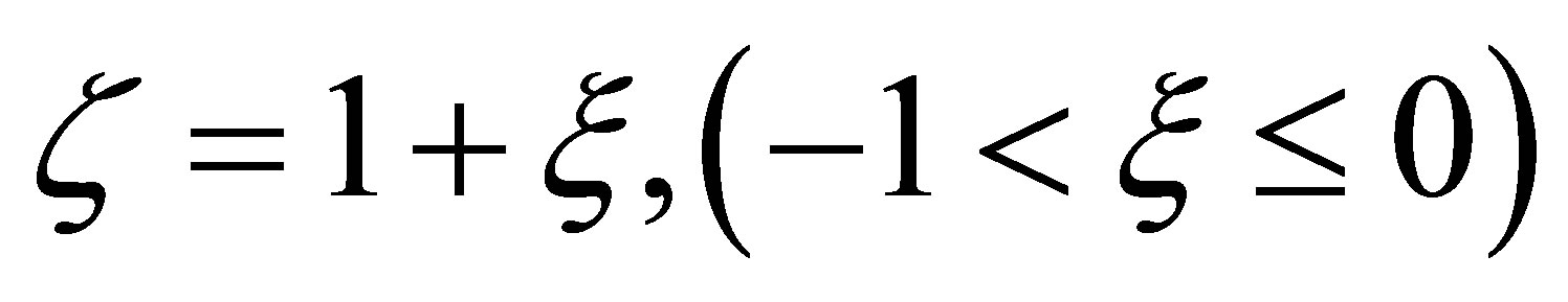 , then we have
 (3.9)
(3.9)
where  is a polynomial of
  with positive coefficients. Hence we have
 (3.10)
Hence, for  sufficiently small we can uniquely solve (3.10). By an implicit function theorem we see that
  is a smooth function of
  such that
  It follows that

Therefore we have (3.4).
Step 4. Next we will prove (3.5). We will solve  namely
 (3.11)
for  Hence we have
 (3.12)
If  does not converges to zero when
 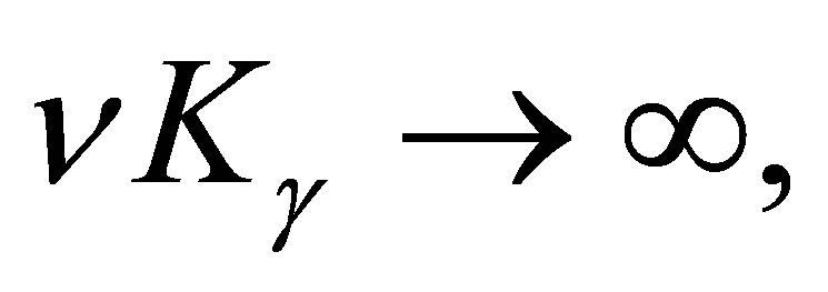 then there exist c>0 and a sequence
 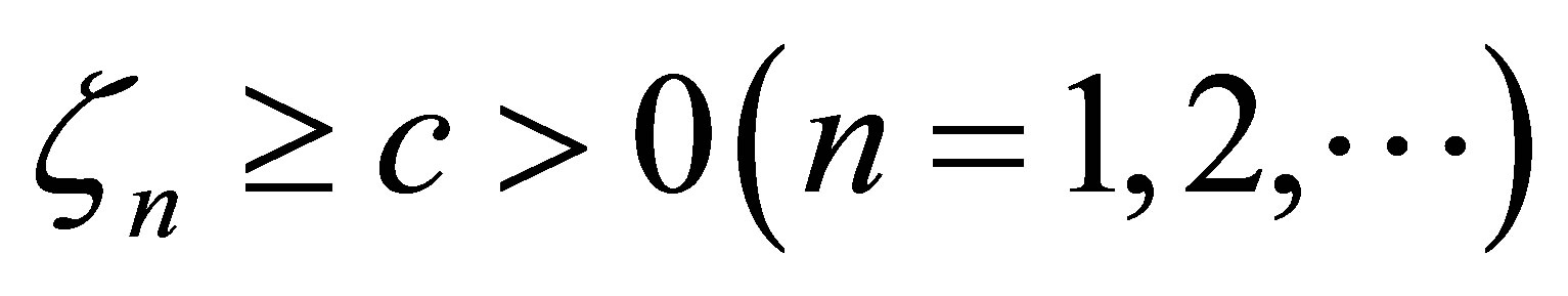 . Since the right-hand side of (3.12) is bounded for
 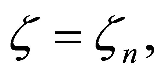 this leads to a contradiction. Hence
  is asymptotically equal to
By solving this relation we have
when  By (3.11) we have
  . It follows that

By simple computations we obtain (3.5).
Step5. If  then we have
 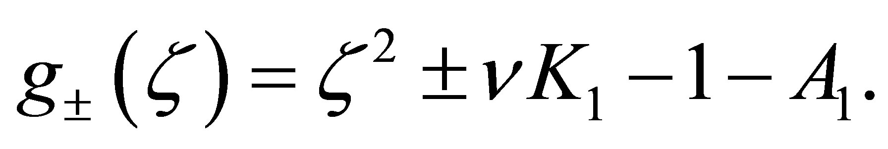 We can easily see that
  on
on 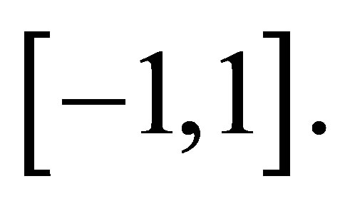 The solution of
 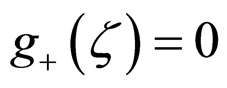 is given by
  The rest of the assertion is almost clear from this formula. This completes the proof.
Remark. We will briefly discuss the difference of dynamics of z in (3.1) for f and  We note that two functions are identical for
  For a small number
 , consider the case shown in Figure 2 for
  Then f looks like as in Figure 3 where new attractive equilibrium points appear near
  because we have made a modification to
  so that
 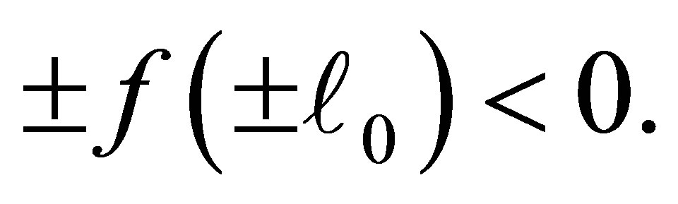 The new equilibrium point corresponds to that of
  with modulus larger than
 . Because of the new equilibrium points we have an apriori estimate of the solution for f. Namely, the orbit started from a neighborhood of the origin does not go beyond
  This fact is important since, if otherwise, the efficiency
  becomes negative. Note that the dynamics of f and
  is the same outside some neighborhood of the boundary
 . We also note that a similar situation occurs in the case
  with
with 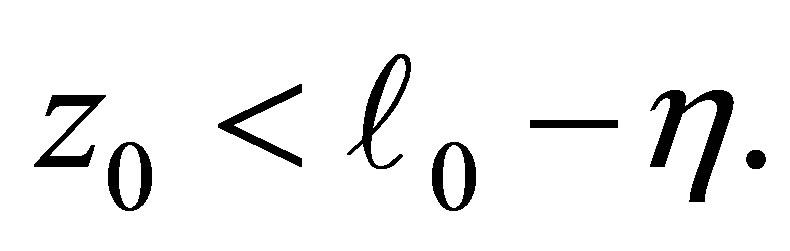 (cf. Figures 1 and 4).On the other hand, if
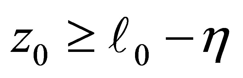 , then the dynamics of f and
  in
in  may be different, while in other part both are the same.
We also note that the apriori estimate holds for f. Therefore apart from the neighborhood of  the dynamics of f is well approximated by that of
 , for which
  we can make concrete analysis of the dynamics, although we do not have the apriori estimate.
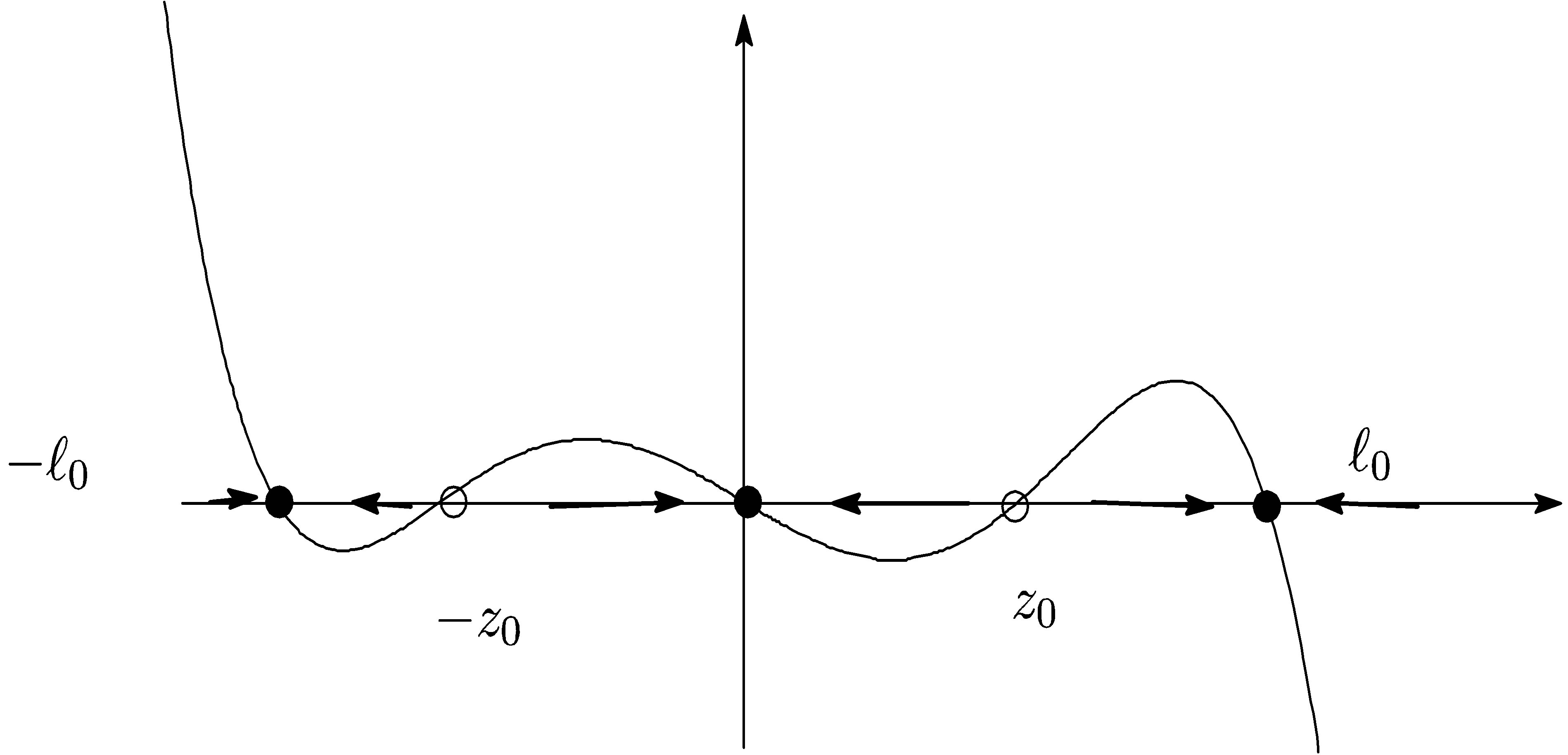
Figure 3. Picture of f. 
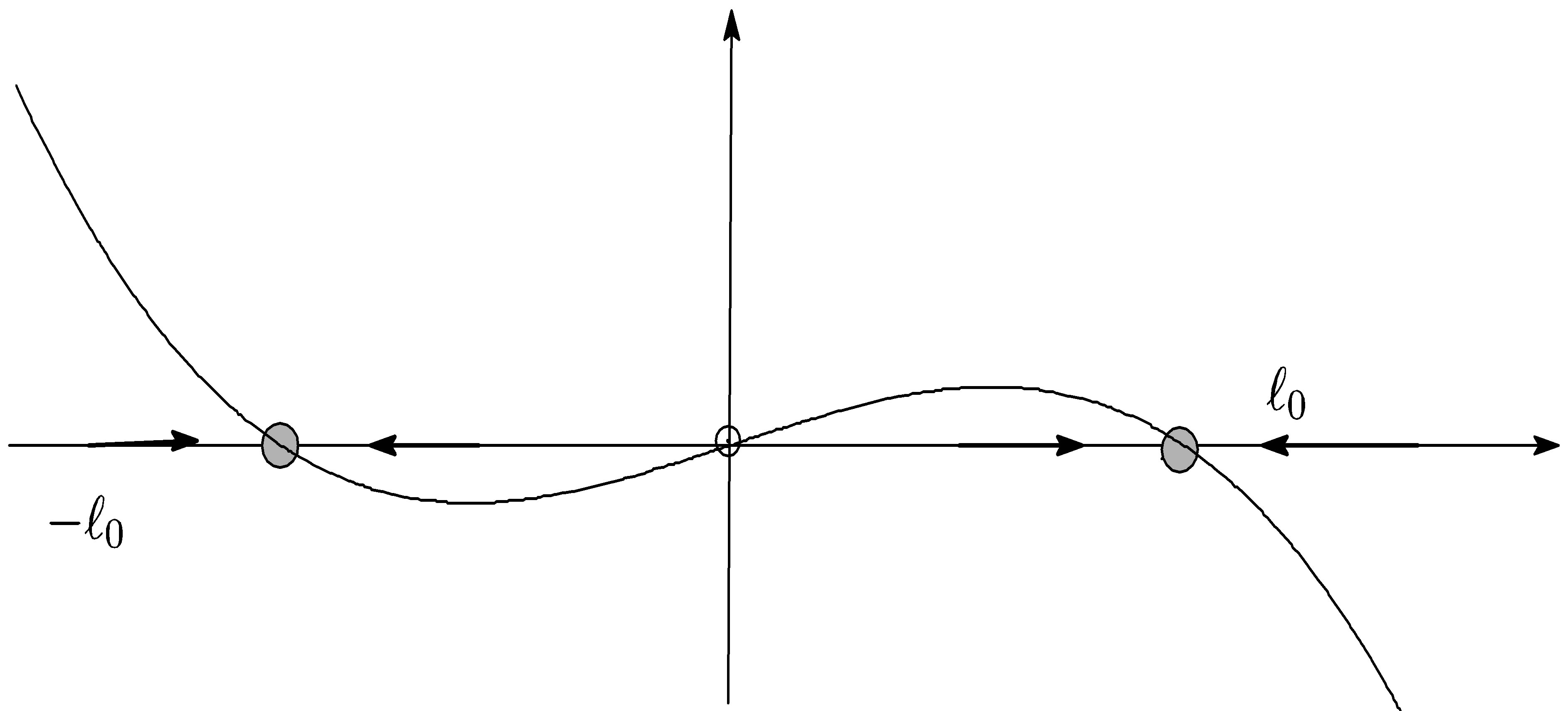
Figure 4. Picture of f. 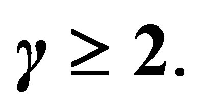
We will study behaviors of solutions under the effect of evolution.
1) Behaviors near the equilibrium point.
We consider how the dynamics of (1.1)-(1.4) is related to the dynamics (1.1)-(1.3) without evolution. We recall that (1.1)-(1.3) without an evolutional effect has what is called a tea-cup attractor. The isocline of (1.1)-(1.3), (3.1) is given by the family of equations
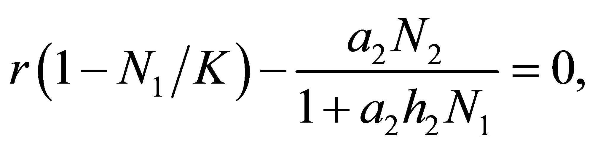 (3.13)
 (3.14)
 (3.15)
 (3.16)
It follows from (3.15) that
 (3.17)
One may assume that A is small since  is small. By (3.14) we have
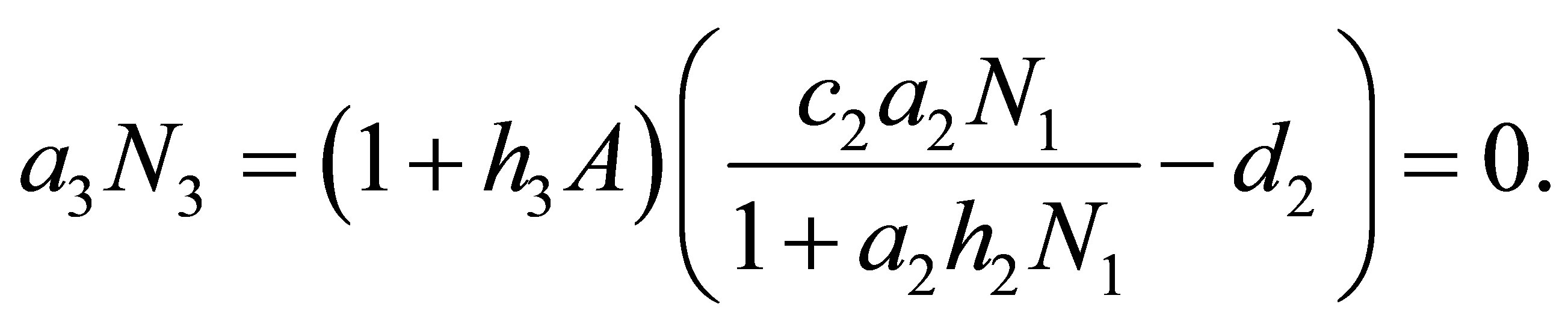 (3.18)
Let us first consider the non-evolutional case, z = 0 or the case where evolution becomes stationary, namely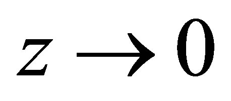 . Then there exists C > 0 such that
  Hence
Hence 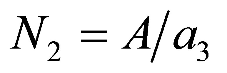 is small and
  is close to K, by (3.13). It follows that there exists
  such that
  if
if  is sufficiently small. In terms of (3.17) and (3.18)
  tends to infinity when
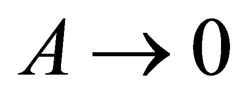 . This implies a typical behavior of
  and
and  around an equilibrium point when there is little effect of evolution. Numerical experiments show that the decrease of
  occurs soon after the orbit approaches to the equilibrium point, namely
  becomes sufficiently large.
Let us consider the evolutional case. Then the main difference from the non-evolutional case is that  may tends to zero. For the sake of simplicity, let us consider the case
  or
or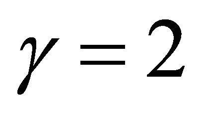 . Assume that there exists an orbit such that
 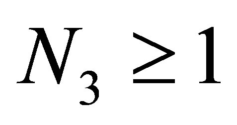 and
and  grows large. Because
  also grows large, it follows from (3.4) that
  tends to zero, and we are in the situation that the orbit of
  tends to
 . Therefore
  tends to zero. Hence the boundedness of
  implies that
  becomes negative. Therefore, by (1.3),
 exponentially decreases. Note that the decrease of
  begins after
  exceeds a certain constant independent of
  and
and  when
when . This exhibits a strong contrast to the non evolutional case where the collapse of
  occurs after
  becomes sufficiently large.
2) Effect of the parameter  to evolution.
In the predatory efficiency  in (C.1)
  represents sensitivity to z. Namely, as
  increases,
  for small z approaches to a constant function. The dynamics of z is quite different in the cases
  and
and . Indeed, if
  and
and

then evolution progresses. (cf. Figure 2 and Figure 3). The latter condition means either the cost of evolution is small,  or
or . We note that the attracttive equilibrium points near
  have the effect to hold the orbits around
 . Conversely, if
  , then we see that fluctuations in progress and rest of evolution takes place.
In the case  we have a different situation. Indeed, if
  then the evolution becomes stationary. If otherwise, then similar fluctuations in progress and rest of evolution as in the case
  takes place. We will show in the next section that in the linear case
  we have a sharp contrast to the case
 .
.
3) Fluctuations of  and
and .
.
The rhythm of  and
and  is also observed in a nonevolutional system and it is related with the structure of a tea-cup attractor. We have a similar phenomenon for an evolutional system.
Let  and
and  be a solution of (1.1)- (1.4). One can show by Poincaré –Bendixon theorem that
  and
and  are an oscillating solution of two species under appropriate choice of parameters. Note that
  tends to zero exponentially. By the continuity of solutions of the initial value problem with respect to an initial value and the apriori estimate of a solution, one can see that for every
  and
and  there exists
  such that if

then

for all  Here, without loss of generality we may assume that the initial time is 0.Especially, this shows that there appears a rhythm of
  and
and  for some interval of time. Note that
  is small and the evolution becomes stationary, i.e.,
 .
.
In order to estimate T, we take ,
,  and
and . By integrating the equation of
 , one has
Hence, if we have
 (3.19)
for sufficiently small , then we have
 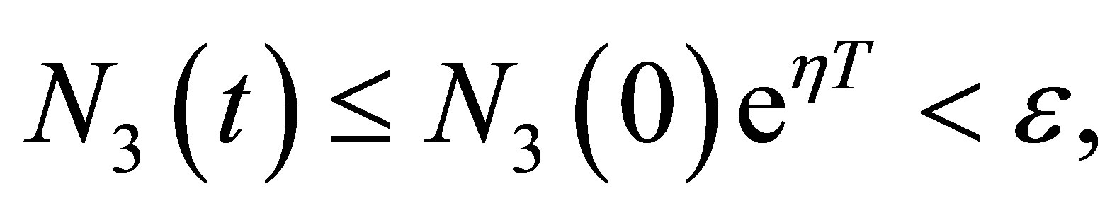 from which we have the estimate of time length T,
 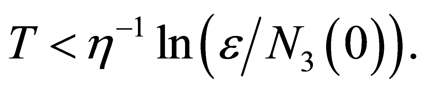 We have a similar condition like (3.19) in the general case
 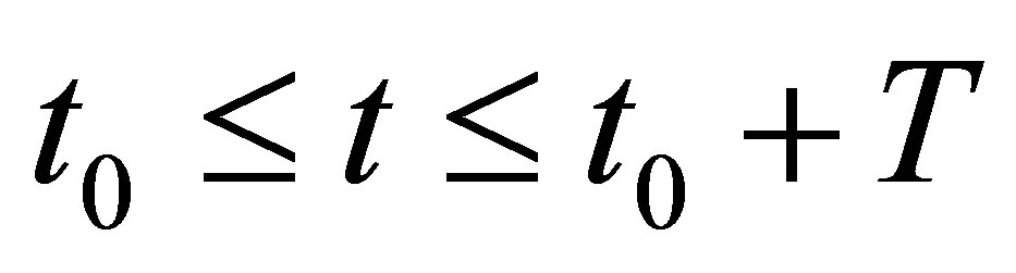 by replacing 0 and T, respectively, by
  and
and  A similar condition like (3.19) holds for some
  and T if we have an averaging property:

4) The limit case when evolution cost tends to zero.
We assume . If the evolution cost tends to zero, namely
  grows from zero to
  , then, by (3.4) and the definition of
 approaches to the origin.
Therefore, the evolution progresses, namely z approaches either of the points . It follows that the predatory efficiency
 . By the same reasoning as in 1)
  tends to zero. We note that in the limit case
  the third species dies out. This agrees with an ecological observation.
4. Evolution for a Linear Predatory Efficiency
We will discuss the evolution in the case
 (4.1)
(4.1)
where  is a real constant and
  .As in the previous case we make modifications of
  in some small neighborhood of the zero point
 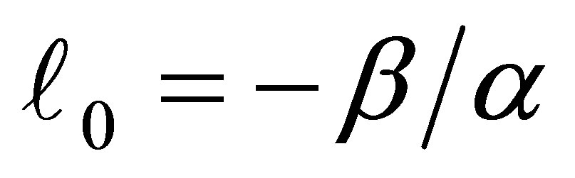 such that
 .
.
For the sake of simplicity, we assume that . By repeating the same arguments as in Section 2 we see that the system of Equations (1.1)-(1.4) with the initial condition (1.6) has a unique global solution in
We will study the dynamics of the evolution in relation with the populations  and
and .We now define
 (4.2)
(4.2)
The condition  is equivalent to
By definition we may consider (4.3) in the set  because, if otherwise,
  Set
Set

and calculate the minimum of  in I. It is taken at
  with the minimum value given by
We recall that  is equivalent to
  Therefore, if
 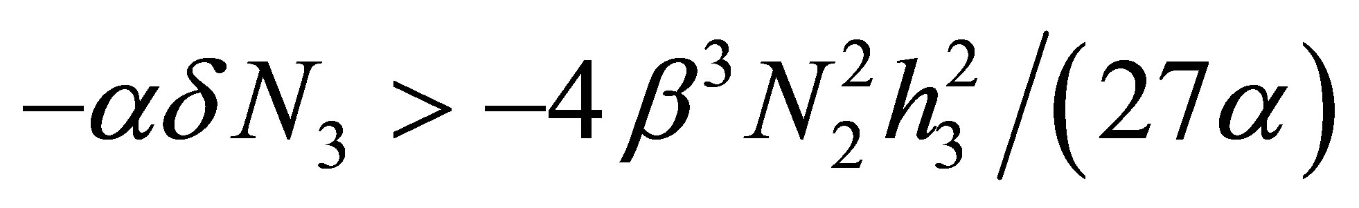 modulo terms of
  namely
 (4.4)
(4.4)
then there appear an attractive equilibrium point  near the origin
 . This means that the predatory efficiency
  is close to a constant function if
  is sufficiently small. Indeed, the equilibrium point
  can be estimated as
In view of the linearity of  and the smallness of
 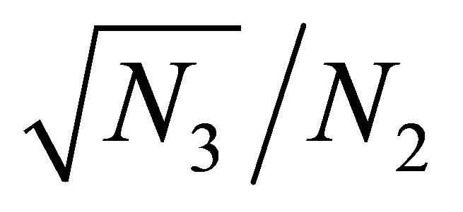 near the equilibrium point we see that
  is almost constant for small changes of
 .
.
Suppose now that (4.4) does not hold. Then the attracttive equilibrium point near 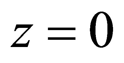 disappears, and there remains an attractive equilibrium point near the zero of
 .Hence the evolution progresses and
  tends to zero. This alternative between the rest and the progress of evolution shows a high contrast to the case of a convex predatory efficiency function discussed in the previous section.
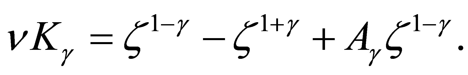
5. Behaviors of Solutions as Cost Increases
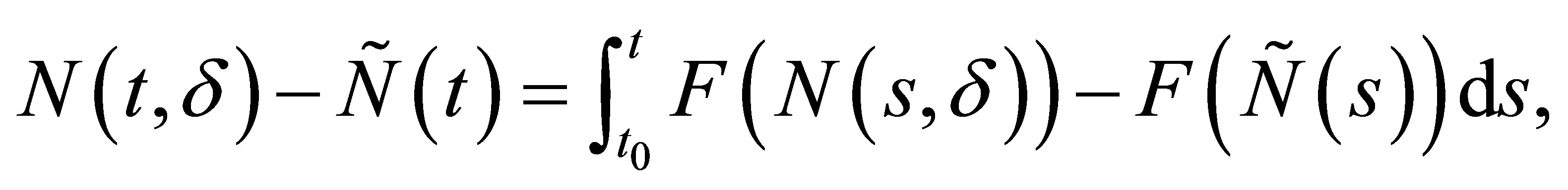
In this section we study the convergence of a solution of an evolutional system to that of a non-evolutional one when the evolutional cost increases, namely  decreases to zero. Let
  and
and  be the solution of (1.1)-(1.4). Let
  be the solution of the non-evolutional system (1.1)-(1.3), namely
  Then we have
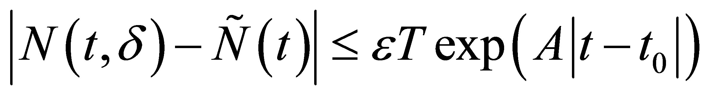
THEOREM 5.1. Assume (2.3). Let  be arbitrarily given. Then we have

uniformly in t on 
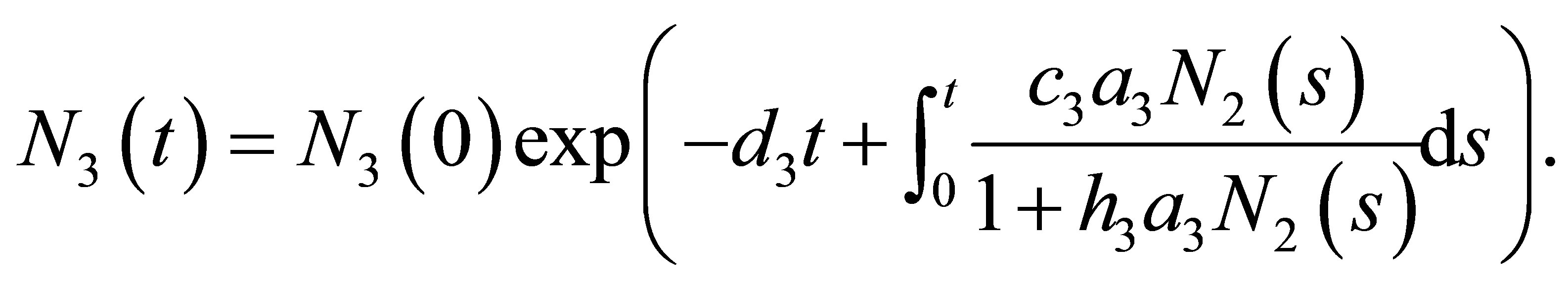
Proof. By integrating (1.4) we have
 (5.1)
(5.1)
If we make the change of variables,  , then we have
 (5.2)
(5.2)
where  and
and
Because  is uniformly bounded in
  by the apriori estimate, it follows that
  times the integrand is uniformly bounded in
  when
when . Hence, the modulus of the integral can be bounded by a constant times
  It follows that
uniformly in  when
when . This entails that
 uniformly in
 .
.
For the sake of simplicity we write (1.1)-(1.3) in
where we use the same notation F as in (2.18). Since
we have
 (5.3)
(5.3)
where the absolute value of a vector means the norm of a vector. Because we have the uniform estimate of  in
in  by (1) of Remark in Section 2, we have

for some  independent of
 .
.
By (1.5) and (5.2) we have
 (5.4)
(5.4)
Because  there exists a constant
  independent of
  such that the right hand side of (5.4) can be estimated by
  It follows that for any
  there exist
  and A>0 such that, for

Therefore we have

By Gronwall’s inequality we obtain, for 
Because  is arbitrary, we have the desired estimate.
6. Discussion
Evolutional Lotka-Volterra system does not seem to be well understood analytically except for the case of two species. In this paper, we have studied how the evolutional change of a character influences global behaviors of a Lotka-Volterra system for three species. We introduced an evolutional equation based on a quantitative genetic model into a Lotka-Volterra system of equations and we proved the existence and the uniqueness of a global solution as well as apriori estimates of a solution. By virtue of these properties, we have given analytical proofs of properties which are different from the nonevolutional system. We hope that some of the properties shown in this paper hold for more general food web settings. It is also interesting to make numerical analysis of our theory in order to understand the effect of evolution. The study of these problems will be left for the future study.
REFERENCES
- R. Lande, “Quantitative Genetic Analysis of Multivariate Evolution Applied to Brain: Body Allometry,” Evolution, Vol. 33, No. 1, 1979, pp. 402-416. http://dx.doi.org/10.2307/2407630
- R. Lande and S. J. Arnold, “The Measurement of Selection on Correlated Characters,” Evolution, Vol. 37, No. 6, 1983, pp.1210-1226. http://dx.doi.org/10.2307/2408842
- P. A. Abrams and H. Matsuda, “Prey Adaptation as a Cause of Predator-Prey Cycles,” Evolution, Vol. 51, No. 6, 1997, pp. 1742-1750. http://dx.doi.org/10.2307/2410997
- P. A. Abrams, “Evolutionay Responses Offoraging-Related traits in Unstable Predator-Prey Systems,” Evolutionary Ecology, Vol. 11, No. 6, 1997, pp. 673-686. http://dx.doi.org/10.1023/A:1018482218068
- P. A. Abrams and H. Matsuda, “Fitness Minimization and Dynamic Instability as a Consequence of Predator-Prey Coevolution,” Evolutionary Ecology, Vol. 11, No. 1, 1997, pp. 1-20. http://dx.doi.org/10.1023/A:1018445517101
- Y. Takeuchi, “Global Dynamical Properties of LotkaVolterra Systems,” World Scientific, Singapore, 1996.
- R. A. Fisher, “The Genetical Theory of Natural Selection,” Claredon Press, Oxford, 1930.
Appendix
(A) The following lemma is used in Section 5.
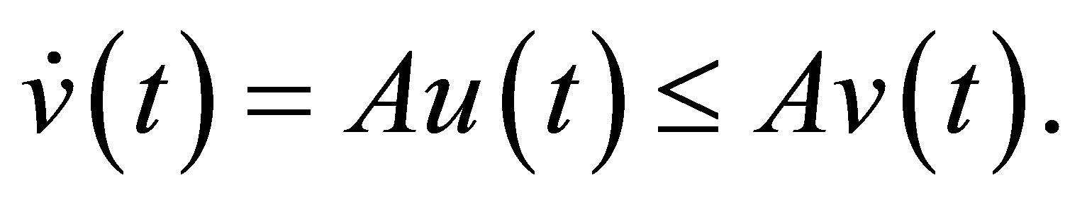
LEMMA. (Gronwall) Let  be a closed interval and let
  Let u be continuously differentiable in I such that, for some constants
  and
and  the inequality
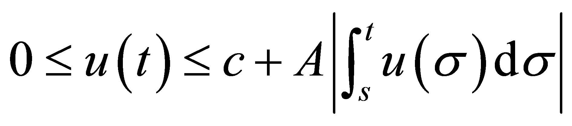
holds true for . Then we have
 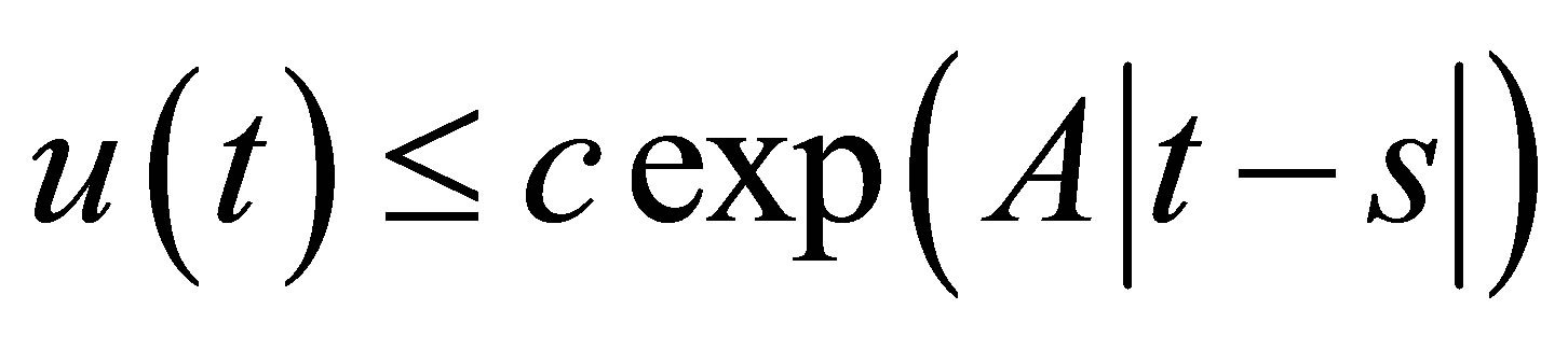 on I.
on I.
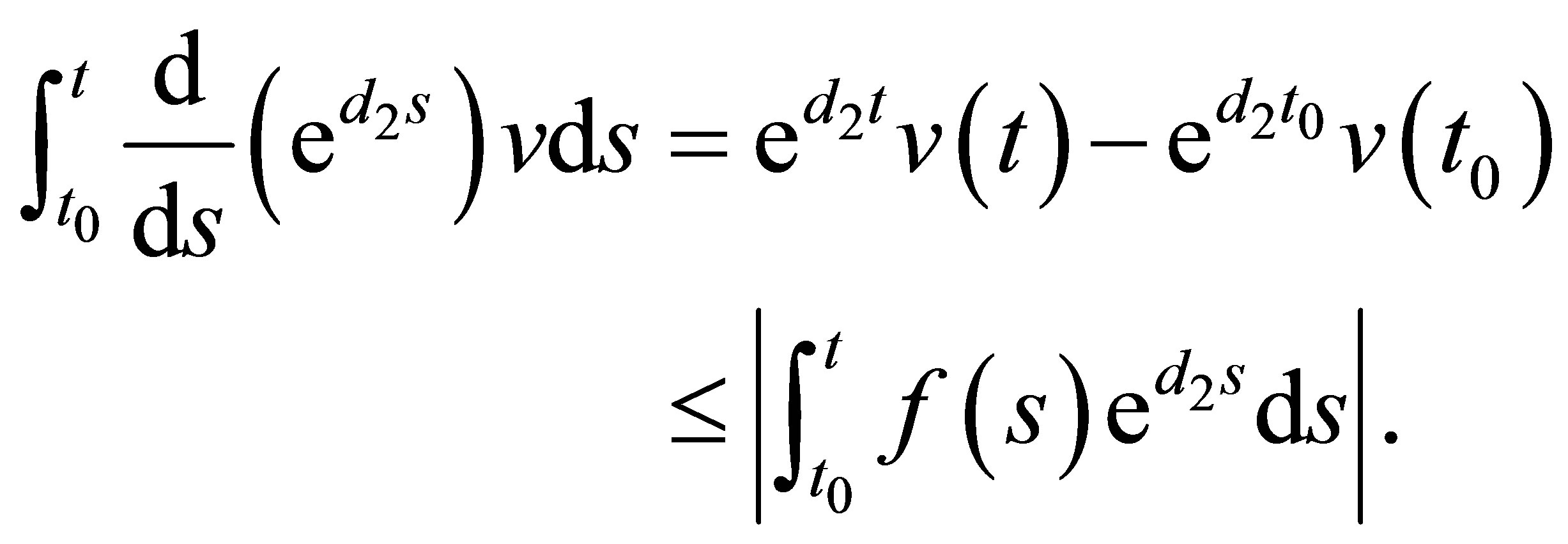
Proof. For the sake of simplicity, we consider the case  Denoting the right hand side of the inequality by v(t) we have the relations,
 and
and
 Multiplying the last inequality with
 , we have
  By integration we get
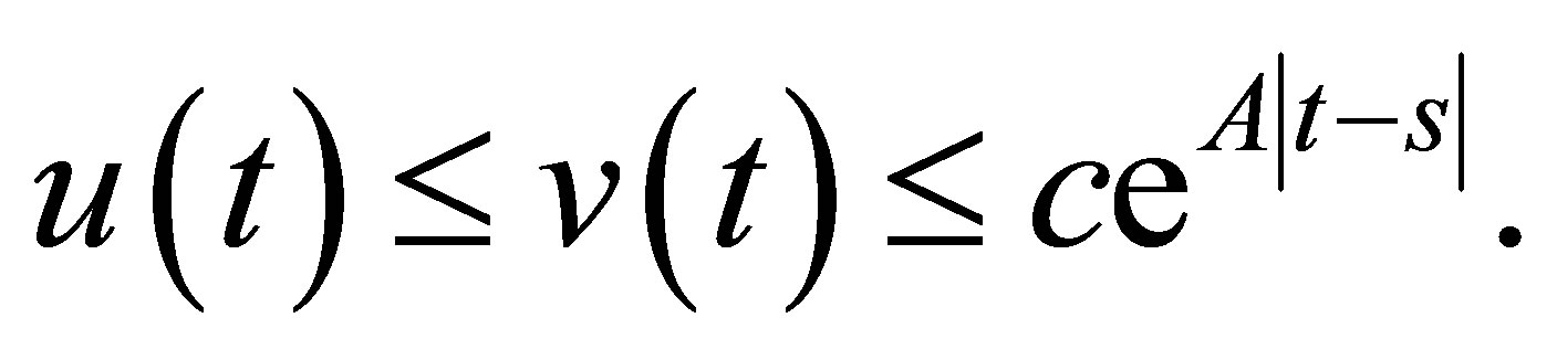
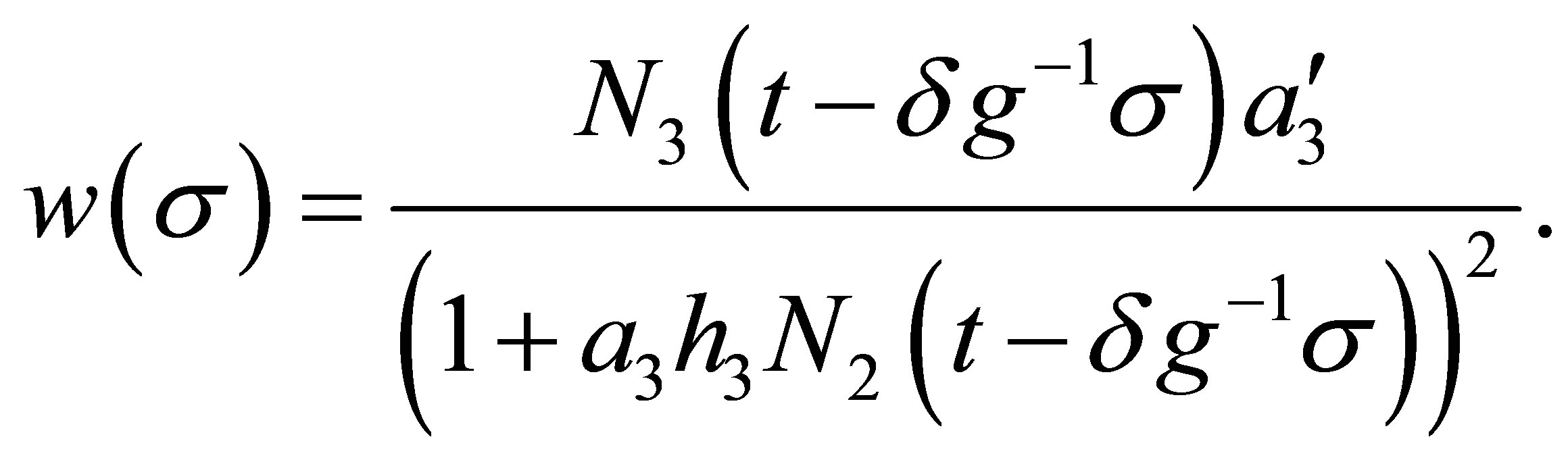
(B) We will briefly show how to deduce (1.4) from the theory of quantitative genetics. Let , g and w be the average character value,the additive genetic variance and the average adaptability of the character value z, respectively. Following the quantitative genetical model we have (cf. [1] and [2]).
The left-hand side is the speed of evolution of a character value. Following Fisher, [7] we have  We assume that (cf. [3-5])

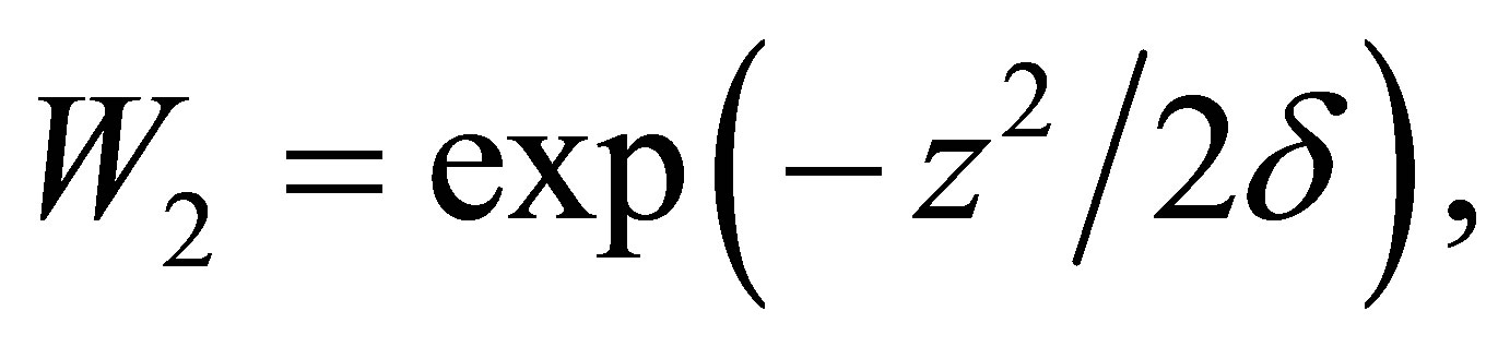
where  is the cost of evolution. By definition we have
 (7.1)
(7.1)
Here ,
,  and
and  are certain constants. We have
Because one may regards  as a constant function when z varies, the right-hand side of (7.1) can be replaced by

Hence we obtain (1.4).