World Journal of Condensed Matter Physics
Vol.2 No.3(2012), Article ID:22141,9 pages DOI:10.4236/wjcmp.2012.23023
Melting of Argon Cluster: Dependence of Caloric Curves on MD Simulation Parameters
![]()
Laboratoire de la Physique de la Matière Condensée (LPMC), Mohammedia Faculté des Sciences Ben M’Sik, Université Hassan II, Casablanca, Morocco.
Email: *tabtimed@gmail.com
Received March 26th, 2012; revised May 16th, 2012; accepted May 27th, 2012
Keywords: Molecular Dynamics Calculations; Clusters; Entropy; Fluctuation; Internal Interaction; Self-Organization; Phase Transformations; Transition; Nanostructures; Melting; Argon
ABSTRACT
We report on molecular dynamics simulations performed using microcanonical ensemble to predict the melting of argon particles in nanometer size range 10 nm and to investigate the effect of the time step integration. We use the LennardJones potential functions to describe the inter-atomic interactions, and the results are evaluated by using caloric curves of the melting phenomenon. Thermodynamic properties, including the total energy, Lindemann parameter, kinetic and potential distribution’s functions, are used to characterize the melting process. The data shows bimodal behavior only in a certain interval of integration time step Δt, while the internal energy increases monotonically with the temperature. For the other time step values, the back bending disappears. We claim that negative specific heat is related to a possible decrease of entropy in an isolated system; this can be interpreted as a result of the internal interactions, especially attractive process and specific relaxation time.
1. Introduction
One of the great challenges in cluster physics in recent years has been the identification and the characterization of critical behaviour and phase transitions, including solidto liquid and liquid-to-gas phase transitions. Since clusters are particles of finite size, one is confronted with the general question of how to detect and/or characterize such a transition in a finite system, a question of interest for many microscopic or mesoscopic systems such as, for instance, melting and vaporization of metallic clusters, Bose condensation of quantum fluids, and nuclear liquidto-gas transition [1-5].
Haberland and co-workers [6] reported the first experimental determination of a caloric curve for the solid-toliquid like transition (melting) of a small cluster, i.e., a sodium cluster ion consisting of 139 atoms. A beam of cluster ions was generated with a canonical distribution of internal energy thus fixing the temperature. One cluster size was selected (thus switching to microcanonical system), irradiated by photons and the photofragmentation pattern (whose positions can be related to the energy) is measured as a function of cluster temperature. Similarly, Bachels et al. [7] reported a caloric curve for a free tin cluster distribution (without mass selection) impinging on a sensitive pyroelectric foil. The interpretation of their experiment was, however, later questioned [8].
Furthermore, Haberland and colleagues [9,10] were able by extending their method to map out the energy distribution of the fragments, demonstrating, by the bimodal shape observed, a possible existence of a negative heat capacity for melting a 147-atom sodium cluster. Haberland and colleagues had, in addition, constructed the caloric curve across the liquid-to-gas like transition [11] using known data of the atomic gas.
M. Farizon and colleagues [12-16] reported experimental measurements of caloric curves for solid or liquid to gas like transition of small charge selected hydrogen clusters. On the other hand, some theoretical and numerical simulations are reported concerning first order transition of argon clusters. In fact, K. L. Nierholz reported the structural and thermodynamic properties of Ar clusters, and derived many thermodynamic properties like caloric heat entropy and internal energy. The obtention of the caloric curves for the microcanonical and the canonical ensemble by molecular dynamics simulations and histogram methods exhibits bimodal behavior (back bending).
The analysis shows that this bimodal behavior is observed only in the case of microcanonical ensemble, while in the case of canonical description, the internal energy increases monotonically with the temperature.
All the reported papers related to the caloric curves present the back bending as a specific property of microcanonical description. For finite size systems, the thermodynamic ensembles are not equivalent.
For macroscopic objects, melting occurs at some well defined temperature; however, this is no longer true for small particles or clusters. At low temperatures, the atoms in a cluster or in a large piece of matter make only small amplitude vibrations around a fixed position. It takes a lot of energy to push an atom from its position in a solid. If the temperature increases, atoms in the cluster can affect neighboring sites and start a diffusive motion.
All properties change with the size of a cluster. The transition from the atom or molecule to the bulk is often quite smooth and the asymptotic behavior well understood. This is not the case for some thermal properties. Large and irregular fluctuations are observed, e.g. in the melting temperature, even for clusters containing several hundred of atoms.
2. Theoretical Approach
According to the Boltzmann’s definition, for an isolated system in equilibrium in microcanonical ensemble (NVE), the entropy is given by [17]
 (1)
(1)
where kB is the Boltzmann constant and Ω(NVE) is the number of discrete microstates in the configurational Г- space consistent with (NVE).
The entropy of any thermodynamic system in equilibrium is given by [18]
 (2)
(2)
where pi is the probability of the microstate i, and the summation is over all possible microstates compatible with the system.
In 1988 Tsallis introduced a new definition for entropy [19,20]
 (3)
(3)
where 0 ≤ q ≤ 1 (q = 1 in the sense of q → 1).
The non extensivity of the entropy observed for small systems is not a consequence of the Tsallis definition. The entropies investigated [21] are all in the framework of the Boltzmann-Gibbs definition. Indeed, all of the non extensivities and non intensities observed in this paper are triggered by conversion of some of the external potential energy into the internal potential energy of the system, an effect that is significant only in small systems.
Entropy, like internal energy, becomes non extensive in small systems. However, there are two differences here:
• First, the non extensivity in the entropy is not as profound as in the internal energy.
• Second, while the internal energy decreases (becomes more negative) due to non extensivity, the entropy increases and, hence, is super extensive.
When two systems are combined, the entropy of the combination of the combined system, Sq(A + B) is given by
 (4)
(4)
If two systems A and B are independent in the sense of the theory of probability, then q = 1 and the entropy is simply the sum of the entropies of its constituents; therefore, the entropy should be an extensive parameter. However, when the systems A and B are dependent, then q < 1 and the entropy as defined by Equation (4) is non extensive, regardless of the size of the system.
Yi-Fang Chang [22] reported that, according to the Boltzmann and Einstein fluctuation theories, all possible microscopic states of a system are equally probable in thermodynamic equilibrium and the entropy tends to a maximum value finally. It is known from statistical mechanics that fluctuations of the entropy may occur [23], while fluctuations always decrease the entropy [24].
When internal interactions exist among subsystems, the statistical independence and equal-probability are unavailable. If fluctuations are magnified [23,24] and the order parameter comes to a threshold value, phase transition will occur. In this case, the entropy may decrease in an isolated system, at least within a certain time. A self-organized structure whose entropy is smaller will be formed.
The Internal Energy of a system is [25] of a system is
 (5)
(5)
where  is the additive part of the particle energy in the state s, in most cases it and E are the kinetic energy; W′ss and U′ss are the absolute values of the attraction and repulsion energies of particles in the states s and s′, respectively.
When the probability changes with time, the entropy of a system composed of two subsystems changes also with time, and the entropy would be defined as [26]:
 (6)
(6)
where . This shows that the entropy decreases with the internal interaction. Not only is this conclusion the same with the conditioned entropy on ρ1 and ρ2, but also it is consistent with the systems theory in which the total may not equal the sum of parts.
3. MD Simulation
The melting-like transition of ArN has been investigated through micro-canonical MD simulations using a LennardJones potential,
 (7)
(7)
where rij is the distance between the particles, and ε and σ are the potential parameters of the LJ potential chosen appropriately to represent particular system of interest, which would be appropriate for solid argon.
The calculations are performed in dimensionless variables by scaling the energy in ε, length in σ, mass in M, temperature in ε/kB, pressure in ε/σ3, time in (Mσ2/ε)1/2.
Here we have chosen M = 0.66 × 10⁻²² g is the atomic mass, and kB is the Boltzman constant. ε/kB = 120 K, σ = 3.84 Å, ε = 1.65324 × 10⁻¹⁴ erg, ε/σ3 = 287 bar and (Mσ2/ε)1/2 = 2.44 ps.
Initially we assign a face-centred-cubic lattice to the positions of the atoms. To start the algorithm, velocities are all set to zero. Sometimes, instead of the velocities being scaled, they are in any case, one has to check the velocity distribution after the equilibration phase has been reached to make sure that it has the equilibrium Maxwell-Boltzmann form. At the end of this equilibration period, all memory of the initial configuration should have been lost.
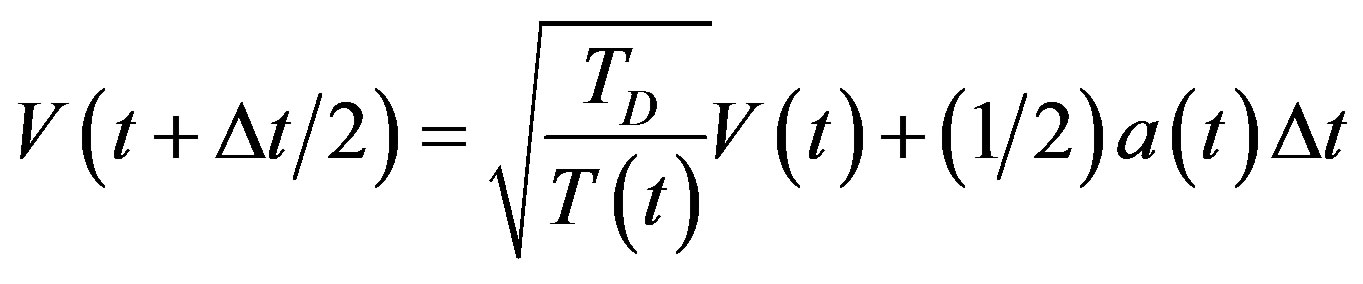
In the present work, we adopt the latter approach to perform molecular dynamics simulations of melting-like transition of ArN, employing the velocity form of the Verlet algorithm [27].
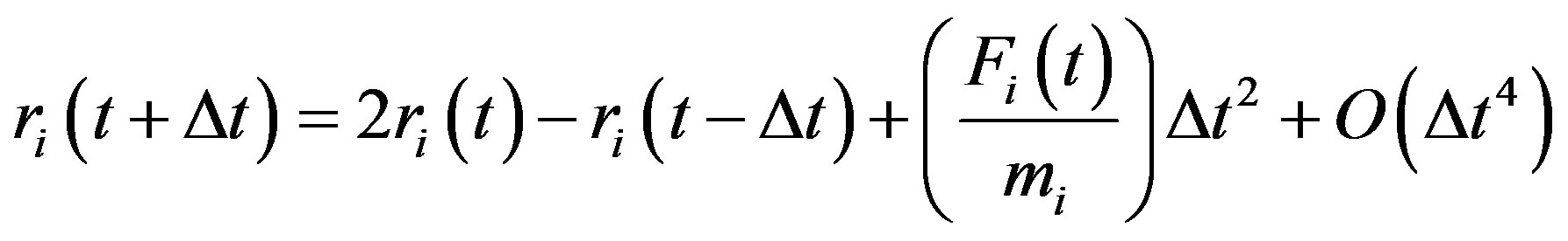 (8)
(8)
The important parameter to choose in an MD simulation is the time increment Δt [28]. In a microcanonical ensemble simulation, the total energy of the system must be conserved. If Δt is too large, steps might become too large and the particle may enter the classically forbidden region where the potential energy is an increasing function of position. This can occur when two particles collide or when a particle hits the “wall” imposed by the external potential. Entering the classically forbidden region means that the new potential energy has become higher than the maximal value allowed. In this case, the total energy has increased, and this phenomenon keeps occurring for large step sizes until the total energy diverges. So, depending on the available total energy, Δt should be chosen small enough so that the total energy remains constant at all times, but not so small that it would require an extremely large number of steps to perform the simulation. The optimal value of Δt is usually found by trial and error. One femto (10−15) second is a good trial guess, but the optimal value really depends on the initial energy and the kind of potential considered.
For the micro-canonical ensemble (constant energy), the mean kinetic energy for different total energies is determined. Then the temperature T is defined by the equipartition theorem; then for practical purposes, it is common practice to define an instantaneous temperature T(t), proportional to the instantaneous kinetic energy EK(t) by a relation analogous to the one above.
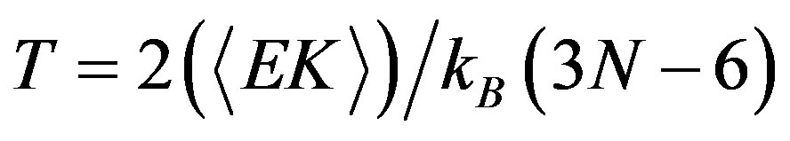 (9)
(9)
With the kinetic energy EK and the number of atoms N, and KB is the Boltzmann constant, and 3N − 6 represents the total number of internal degrees of freedom.
The total internal energy of a system can be written as a sum of kinetic and potential energy contributions, and the temperature of the system is proportional to its average kinetic energy.
The cluster’s configuration has a lower configurational energy EP which nearly compensates the effects of the potential truncation at 2.5σ.
Temperature changes are usually achieved by enabling a device in the code that brings the system to the desired temperature TD by rescaling the velocities. In the velocity verlet algorithm discussed at the end of this may be accomplished by replacing the equation
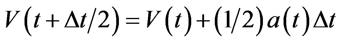 (10)
(10)
by
 (11)
(11)
where TD is the desired temperature, and T(t) the instantaneous temperature.
Switching to liquid-like state it is increasing its configurational energy; hence the kinetic energy has to be reduced to keep the total energy constant. Because of this, the same mean kinetic energy can be obtained at different total energies.
An observable commonly studied in the context of melting transitions is Lindemann’s parameters <δ> [29],
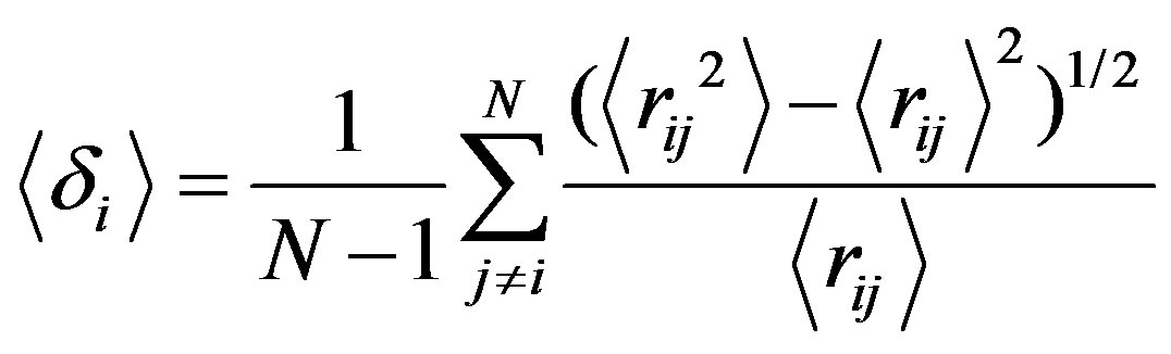 (12)
(12)
where N is the number of molecules in a cluster and rij is the distance between ith and jth Argon atoms.
This parameter measures the root mean square of the distance between two atoms averaged over all pairs. Even short isomer fluctuations with a subsequent return to the ground state can leave the cluster reordered; i.e., a previously nearest neighbour pair rij may become a secondor third-neighbour pair after the fluctuation. Such a reordering leads to a notable increase in , allowing for the clear identification of a melting transition. Note that the Lindemann criterion of melting, which measures the atomic fluctuations with respect to their equilibrium positions, is usually employed for bulk systems but is less well suited for cluster systems.
The second observable of interest is the specific heat, which can be obtained from the thermodynamic averages of the potential energy EP and its square.
The second observable of interest is the specific heat, which can be derived from the total energy expression.
4. Simulation Results
During the first 2500 MD steps, for N = 256 Argon atoms, positions are defined on a lattice assuming CFC crystal structure witch correspond to the most stable one at T = 0 with Leonnard Jones potential. Initial velocities have been taken to be zero, or are assigned taking them from a Maxwell distribution at a certain temperature T.
To ensure a reasonable numerical stability, the basic time increment is taken to be Δt = 0.008. The actual time will be fairly small since only a limited number of integration steps are possible.
Of course, such an initial state will not correspond to an equilibrium condition. However, the steady state is reached after a time of the other of 500 time steps Δt (Δt = 0.008), and one should wait for the system to reach equilibrium under clean constant energy conditions before collecting data. 1000 additional time steps are needed to determine the mean values of the calorific curve, heat capacity, root-mean-square (RMS) bond length fluctuations, and melting temperatures corresponding to the desired temperature TD = 1.3476. The system is driving to this desired temperature by rescaling the velocities in the velocity Verlet algorithm in order to keep the system under control. All quantities are given in reduced units.
For Δt = 0.008 and at the indicated desired temperature TD, the kinetic energy distribution of the N Ar atoms is plotted in Figure 1. This curve exhibits Maxwell distri-
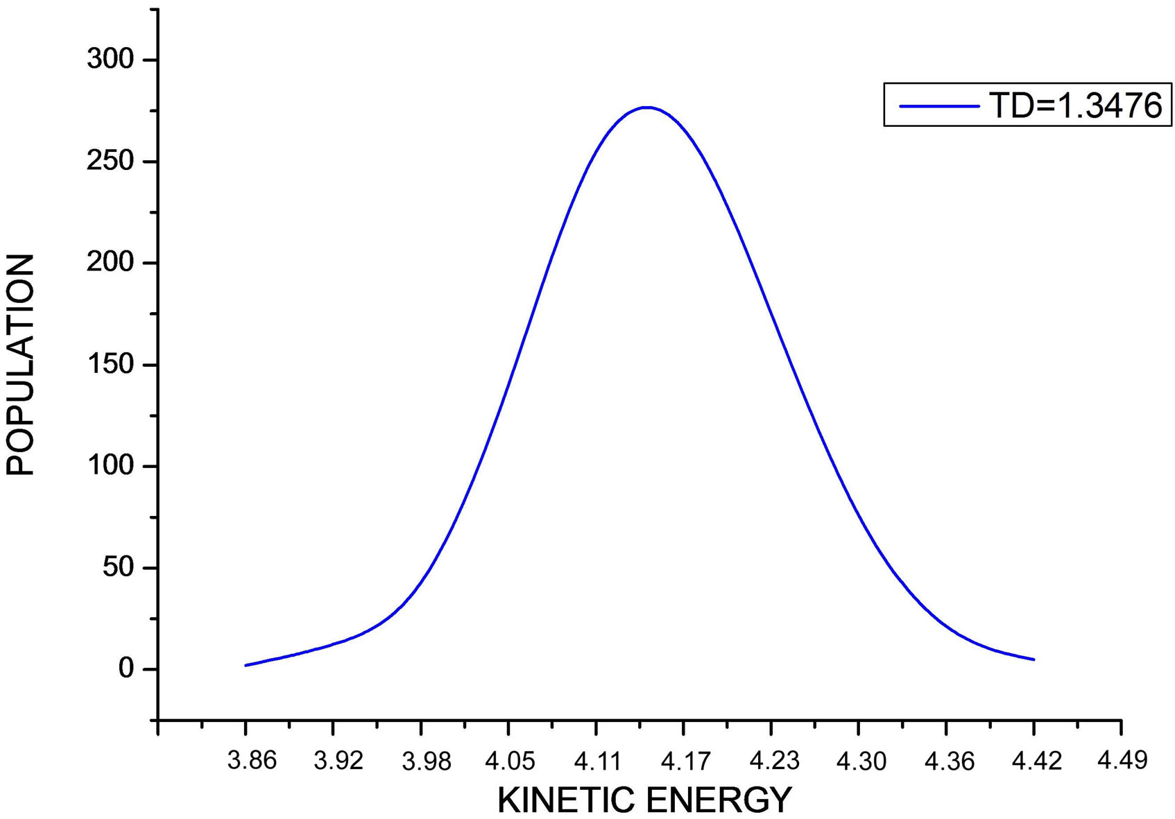
Figure 1. The figure shows the distribution of the kinetic energy values during the simulation at indicated desired temperature.
bution shape.
For a step of integration Δt = 0.008 and then by varying the temperature ΔTD = 0.5, for each value of the temperature TD are averaged physical quantities such as temperature, kinetic energy, potential energy, total energy, specific heat, and Lindemann factor. Then we draw for integration step Δt = 0.008 in Figure 2 the evolution of the average kinetic energy, potential, and total according to the desired temperature.
Starting from T = 0, the caloric curve increases roughly linearly, but near the melting temperature there is an acute change in slope characterized by a sudden jump analogous to bulk melting behavior. This jump is expected to be smoothed to a finite with small systems [27-30].
In our case, we observe that this jump occurs at the reduced temperature Tmelt (Tmelt =1.45) which corresponds to 174 K considered as the liquid-solid transition.
According to the study by Lutsko et al. [31], a factor should be introduced between the simulated structure of an isolated cluster and the actual (thermodynamic) melting points when periodic boundary conditions are enforced for bulk materials. The thermodynamic melting point is approximately 1.4 - 1.5 times its structural counterpart.
For a given same values of the integration time step, we observe, in addition, that the microcanonical internal energy exhibits an S-shaped curvature in the coexistence region where both solid-like and liquid-like states can occur. This can be understood by considering the constant energy ET = EP + EK, the cluster switches between solid and liquid along time scale. In solid-like state, the configuration of the cluster has a lower configurational energy. Switching to a liquid-like state, it is increasing its total energy; hence, the kinetic energy has to be reduced to keep the total energy constant. Because of this, the same mean kinetic energy can be obtained at different total energies.
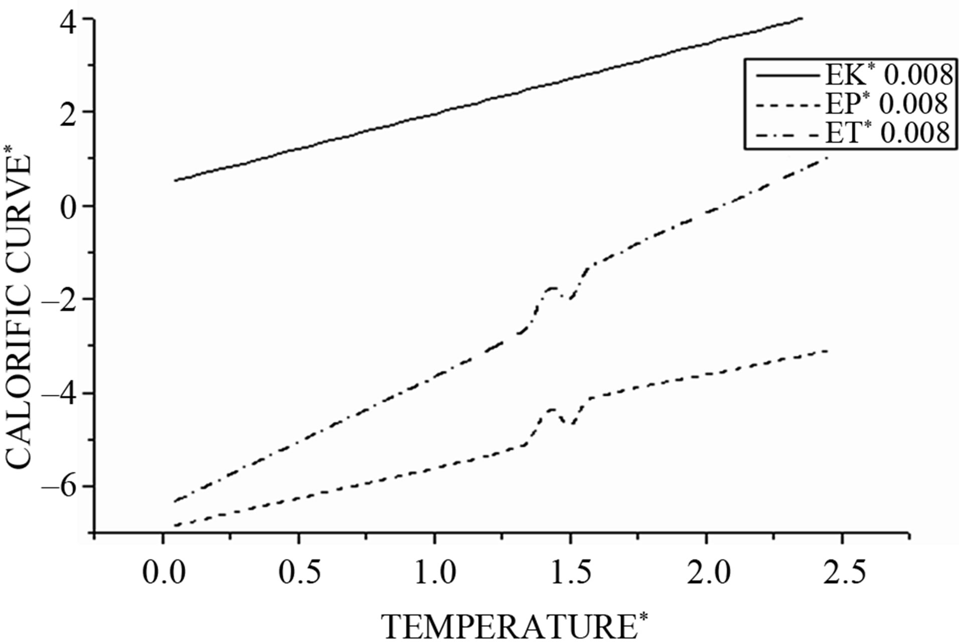
Figure 2. Shows the kinetic (EK), potential (EP) and total energy (ET) as function of the cluster temperature.
With , we have three regions;
Region I 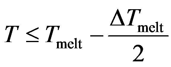
Region II 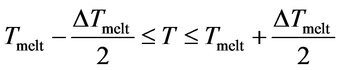
Region III 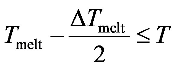
The potential curve is characterized by two distinct parts, where the solid part corresponds to Region I and the liquid part to Region III. Those two parts are separated by a gap  in which the cluster fluctuates between the two phases; this region of coexistence of solid and liquid phases represents two behaviors where the potential energy distribution has a dent with an inverted curvature, and shows a bimodal structure.
Then the change in the potential energy can be interpreted as responsible for this back bending phenomenon.
Then we draw for integration step Δt = 0.008 in Figure 3 the evolution of the average specific heat according to the desired temperature. In the transition region, we observe a double peak structure that also can be interpreted by the coexistence of the solid and the liquid phase.
In our simulations of melting, we monitor the phase changes of clusters using atom-resolved root-mean-square (RMS) fluctuation of the interatomic distances.
For the solid state, in which atoms are fixed in lattice sites, the value of this parameter is typically smaller than 0.1, considerably smaller than that for the liquid state with its mobile atoms. This parameter corresponds to a time scale in which atomic transitions between sites for the solid cluster state are improbable, while these transitions for the liquid cluster state are effective.
Figure 4 demonstrates this for the 256-atom LennardJones cluster with the argon pair interaction parameters.
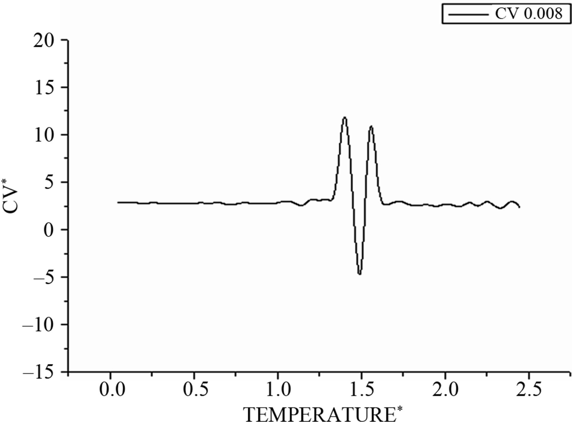
Figure 3. Shows the corresponding heat capacity obtained by the derivative of the total energy on the temperature.
One can see that the (RMS) curves increase slowly with the temperature but beyond the point  increases fastly and fluctuates before reaching the mean value corresponding to the liquid steady state. So this parameter has a jump in the vicinity of the cluster melting point
 , and the point of inflection of this jump may be used as the definition of the melting point. However, because the “jump” clearly takes place over a finite temperature interval, the melting point of the cluster becomes more subjectively defined; e.g., the point of inflection of this curve, or the point of equal chemical potentials of the two phase-like forms. Often, the term “melting point” of a cluster is taken to be the condition at which the free energies of the two phases are equal.
In this (RMS) fluctuating region, the global cluster system can be interpreted as subdivided into two arbitrary interacting subsystems. The total internal energy of the cluster is not simply the sum of individual internal energy of the subsystems. We have to take into account an additive term due to the interaction between the subsystems that makes that internal energy at the melting point not an extensive quantity.
5. Caloric Curves Dependence on MD Simulation Parameters
To test the effect of varying the time increment Δt, the value of physical quantities, so for a definite value to the desired temperature, the simulations were performed for different values of the time increment from 0.01 to 0.009 with an infinitesimal change in the order of 0.0005. Each simulation was performed for the same total time of 1500 time steps or stages, and the raw sampled data for the quarter of the initial time interval of the simulation was excluded from subsequent analysis. In order to monitor the equilibration process, the overall temperature kinetics, heat capacity, Lindmann factor, and the energy (kinetic, potential, and total) were recorded.
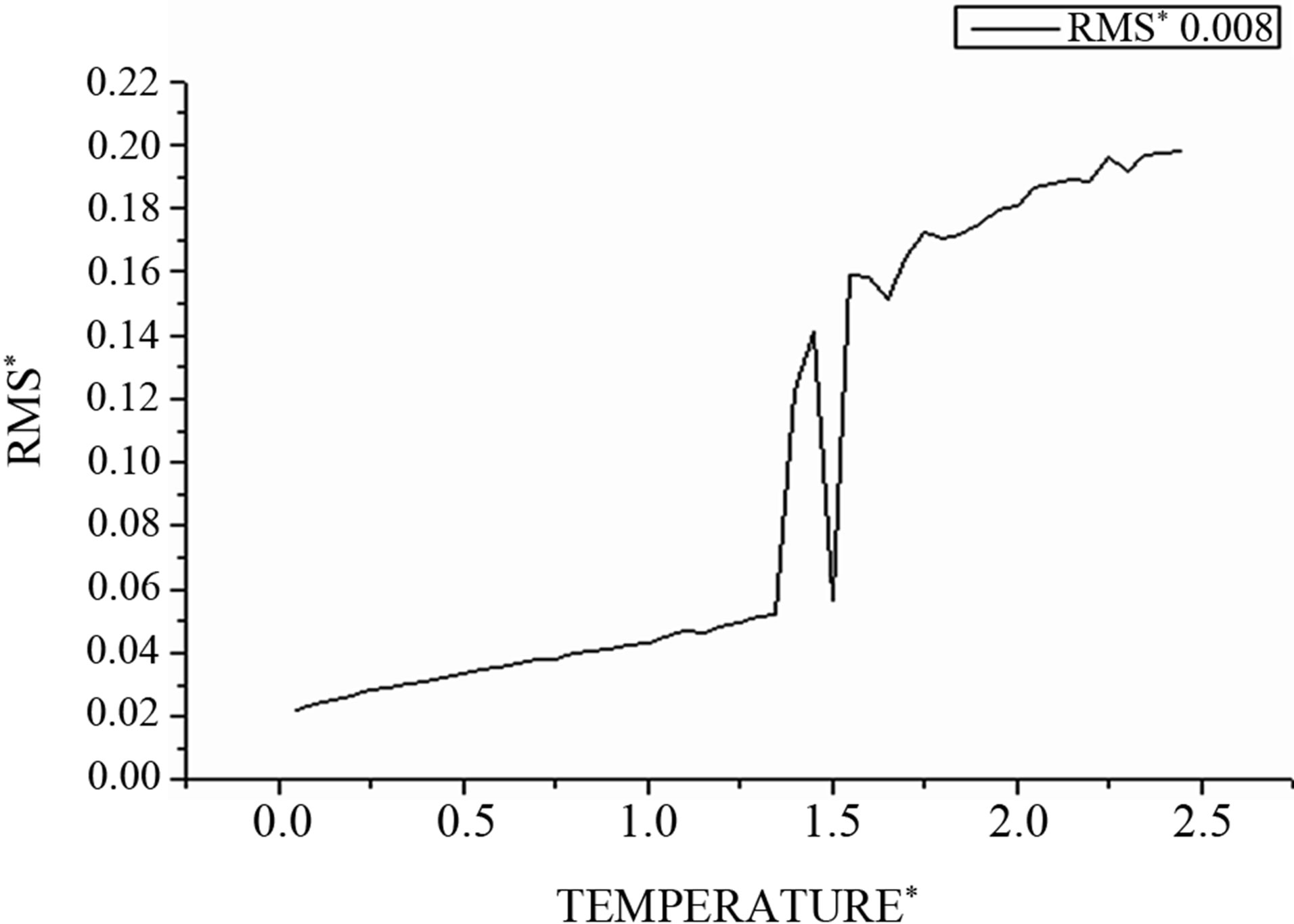
Figure 4. The RMS as function of temperature.
Figure 5: In this figure, we note for all values of integration step Δt with (Δt = 0.0076; 0.0078; 0.008) that all curves of kinetic energy are superposed and proportional to the values of temperatures, so the evolution of the kinetic energy function is independent from a different values of Δt.
On the other hand, all curves of total energy are superposed in two regions I and III; however, between them, curves exhibit an S-shaped curvature in the coexistence region where both solid-like and liquid-like states can occur depending on the integration time step Δt.
For Δt = 0.0078 and Δt = 0.008 we observe back bending (S-shaped curvature).
For the other values like Δt = 0.0076 the total energy, or in similar manner the potential energy, increases monotonically with temperature and the back bending disappears.
In the same manner, the heat capacities in Figure 6 show a bimodal behavior that is missed by changing the values of integration time step Δt.

Figure 5. The kinetic, and total energy as function of temperature at different values of time of integration step Δt.

Figure 6. Shows the corresponding heat capacity obtained by the derivative of the total energy on the temperature.
The curves in Figure 7 effectively show that the distance between atoms increases slowly with the temperature; when the temperature becomes greater then the distance increases swiftly until a value where the system becomes unstable. At this point, the system can be subdivided into arbitrary subsystems, between which interactions must be taken into account, regardless of their small size. Energy between these systems is not an extensive quantity because the total energy is not simply the sum of the energy of the subsystems.
Considering its non-extensitivity, to avoid partly molten states, a reduced system prefers to convert part of its kinetic energy into potential energy in its place. Consequently the cluster can become colder, where its total energy increases; the distance then decreases to find stability before quickly increasing.
In Figure 8, we draw the curve representing the distribution of particle number according to kinetic energies during the simulation at different values of temperature. We note that all curves are superposed and have a shape of a centered Maxwell distribution.
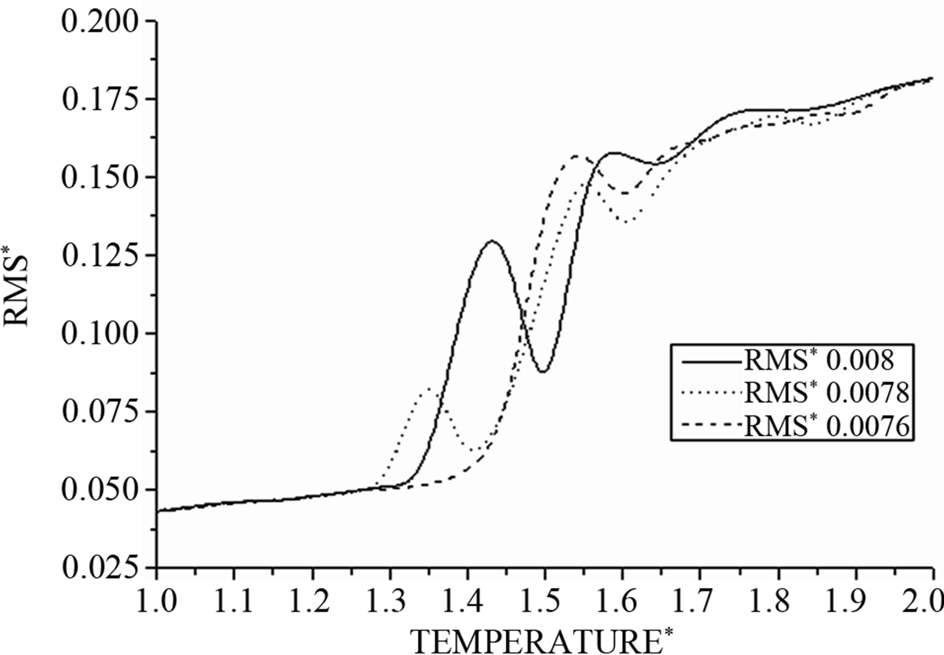
Figure 7. The RMS as function of temperature at different values of time integration step Δt.
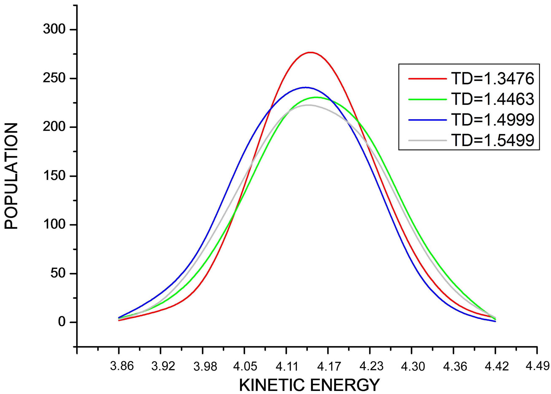
Figure 8. Shows the Maxwell distribution of the kinetic energy values during the simulation at different values of desired temperature.
In Figure 9, the curve represents the distribution of particle number according to potential energies during the simulation at different values of temperature.
We distinguish two different cases:
• When the internal energy is monotonic, or similarly, when the heat capacity exhibits one peak, all the potential energy distributions are superposed.
• When the internal energy is monotonic or similarly.
When the heat capacity exhibits bimodal behavior (back bending), the potential energy distributions are shifted to higher energy value that corresponds to a decrease of the (RMS) and signals the occurrence of attractive interaction governing the process.
Note that all curves are superposed and have a shape of a centered Maxwell distribution, but the curve corresponding to TD = 1.4463 is higher, decaled, and not symmetric like the other curves.
We conclude that upon melting, the kinetic energy, and thus the temperature, remains constant. A small system tries to avoid partly molten states and prefers to convert some of its kinetic into potential energy instead. Therefore, the cluster can become colder while its total energy increases.
6. Discussion
In the equilibrium thermodynamic, all possible microscopic states of a system are equal probable and the entropy tends toward a maximum value; finally, many fluctuations occur, decreasing the entropy.
The internal interactions in certain conditions can magnify these fluctuations.
In this study, simulations have been performed with an integration step Δt, which is good enough to maintain the energy constant for relatively short runs of about 1000 integration steps. Because we need long runs to observe dynamical coexistence, we have tested the ability of this algorithm to maintain the total energy as a function of the

Figure 9. Shows the Maxwell distribution of the potential energy values during the simulation at different values of desired temperature.
time step Δt of integration. For longer runs, the accuracy rapidly decreases. A very small Δt would maintain the energy much better, but the computation time would become unrealistically long, and, worse still, the truncation errors start to play an important role. Hence, the choice of Δt should simultaneously satisfy two requirements:
• To be much shorter than the characteristic time;
• and to be large enough to make the computations efficient.
A straightforward argument makes clear why and how the effective heat capacity of a microcanonical ensemble, defined in terms of the mean kinetic energy, may be negative. The phase-like forms of clusters are interpreted in terms of states where clusters reside depending on their surface potential energy.
Clusters in liquid states reside on a sort of large hollows with small barriers, so that the atoms can move rather readily through many conformations. In this later case, the mean potential energy is high relative to the bottom of the well corresponding to the solid. At low energies, the system cannot escape the deep minimum, and is therefore solid. This situation means that at high enough energies, the cluster moves between these two forms of potential essentially as readily as it moves potential surface of liquid.
The question now is: at which ranges of energy (or temperature) are the solid and liquid states recognizable?
The response is that the systems must spend intervals long enough in each region to develop properties characteristic of each state. Hence, there must be enough of a barrier that separates the solid and liquid regions of the potential surface to yield those sufficiently long dwelling times.
As the total energy of the cluster increases, it spends a larger fraction of time in the liquid region, which has high potential energy and low kinetic energy.
Increasing the energy allows the system to climb into regions of ever-increasing potential energy, while the average kinetic energy of the liquid may remain low, even as its total energy increases. This explains clearly the situation in which increasing the energy of the system lowers the mean kinetic energy, and thereby lowers the kinetic temperature.
We believe that the potential type and the transition time between different configurations that are principally related to the dwell time of the system in a given conformation are responsible of the back bending behavior.
According to Yi-Fang Chang [32], attractive process is one of internal interactions that can magnify a fluctuation. For example, in an isolated system of n constituents which are in different states of energy. Ωn: Number of the possible states of the system.
Now, if we consider that internal attractive interaction exists in system the n-constituents’ cluster to m-aggregates, each aggregates in a finite number of initial constituents.
 (13)
(13)
And
 (14)
(14)
m < n for the condensed process, entropy decreases dS < 0. Conversely, m > n for the dispersed process.
The argon melting cluster can be interpreted in terms of the coexistence of two subsystems with internal interactions. In this picture the internal energy and the entropy will not be additive extensive quantities.
7. Conclusions
How can this negative heat capacity be interpreted? Upon melting, a large system converts added energy completely into potential energy, reducing continuously the fraction of its solid phase. The kinetic energy, and thus the temperature remain constant. A small system, on the other hand, tries to avoid partly molten states and prefers to convert some of its kinetic energy into potential energy instead. Therefore the cluster can become colder, while its total energy increases.
In our study, the most important condition for detecting coexisting phases is the rate of cooling-heating which must be large in comparison to the relaxation time.
In the region of the phase transition, depending on the value of integration step, the system may or may not be stable. If the system is unstable due to the competition between its subsystems, the dominance of attractive forces will cause the appearance of the back-bending phenomenon.
As pointed out by Berry [33], a rugged potential energy surface requires a slow enough change of the system’s temperature to avoid trapping it in a metastable state. If this trapping happens, the system cannot escape from a local minimum for realistic computational times.
Effectively we have demonstrated that for a given intervals of time step integration, due to the nature of LJ potential, the structure of configurational states of Ar clusters varies significantly with increasing cluster temperature, and new configurational states come into play in the liquid state as the cluster is excited. This is accompanied by a significant energy gap between the solid and liquid.
REFERENCES
- F. Gulminelli and P. Chomaz, “Critical Behavior in the Coexistence Region of Finite Systems,” Physical Review Letters, vol. 82, no. 7, 1999, pp. 1402-1405. doi:10.1103/PhysRevLett.82.1402
- M. D’Agostino, et al., “Nuclear Liquid-Gas Phase Transition: Experimental Signals,” Nuclear Physics A, vol. 749, 2005, pp. 55c-64c. doi:10.1016/j.nuclphysa.2004.12.008
- P. Chomaz and F. Gulminelli, “The Challenges of FiniteSystem Statistical Mechanics,” The European Physical Journal A, vol. 30, no. 1, 2006, pp. 317-331. doi:10.1140/epja/i2006-10126-5
- D. H. E. Gross, “Microcanonical Thermodynamics: Phase Transitions in ‘Small’ Systems,” World Scientific, Singapore, 2001.
- D. H. E. Gross, “Micro-Canonical Statistical Mechanics of Some Non-Extensive Systems,” Chaos, Solitons & Fractals, vol. 13, No. 3, 2002, pp. 417-430. doi:10.1016/S0960-0779(01)00023-6
- M. Schmidt, et al., “Experimental Determination of the Melting Point and Heat Capacity for a Free Cluster of 139 Sodium Atoms,” Physical Review Letters, vol. 79, No. 1, 1997, pp. 99-103. doi:10.1103/PhysRevLett.79.99
- T. Bachels, et al., “Melting of Isolated Tin Nanoparticles,” Physical Review Letters, vol. 85, no. 6, 2000, pp. 1250-1253. doi:10.1103/PhysRevLett.85.1250
- R. Kofman, et al., “Melting of Isolated Tin Nanoparticles,” Physical Review Letters, vol. 86, no. 7, 2001, pp. 1388-1392. doi:10.1103/PhysRevLett.86.1388
- M. Schmidt, et al., “Negative Heat Capacity for a Cluster of 147 Sodium Atoms,” Physical Review Letters, vol. 86, No. 7, 2001, pp. 1191-1194. doi:10.1103/PhysRevLett.86.1191
- M. Schmidt, et al., “Caloric Curve across the Liquidto-Gas Change for Sodium Clusters,” Physical Review Letters, vol. 87, 2001, Article ID: 203402. doi:10.1103/PhysRevLett.87.203402
- M. Schmidt and H. Haberland, “Agrégats Comme Pré- curseurs des Nano-Objets Clusters as Precursors of NanoObjects,” Comptes Rendus Physique, vol. 3, 2002, pp. 327-340. doi:10.1016/S1631-0705(02)01326-9
- F. Gobet, et al., “Cluster Multifragmentation and Percolation Transition. A Quantitative Comparison for Two Systems of the Same Size,” Physical Review A, vol. 63, No. 3, 2001, Article ID: 033203. doi:10.1103/PhysRevA.63.033202
- F. Gobet, et al., “Probing the Liquid-To-Gas Phase Transition in a Cluster via a Caloric Curve,” Physical Review Letters, vol. 87, No. 20, 2001, Article ID: 203401. doi:10.1103/PhysRevLett.87.203401
- F. Gobet, et al., “Direct Experimental Evidence for a Negative Heat Capacity in the Liquid-to-Gas Phase Transition in Hydrogen Cluster Ions: Backbending of the Caloric Curve,” Physical Review Letters, vol. 89, No. 18, 2002, Article ID: 183403. doi:10.1103/PhysRevLett.89.183403
- B. Farizon, et al., “Direct Observation of Multi-Ionization and Multifragmentation in High Velocity Cluster-Atom Collision,” Chemical Physics Letters, vol. 252, 1996, pp. 147-152. doi:10.1016/S0009-2614(96)00125-X
- M. Farizon, B. Farizon, S. Ouaskit and T. D. Mark, “Fragment Size Distributions and Caloric Curve in Collision Induced Cluster Fragmentation,” American Institute of Physics, vol. 970, 2008, pp. 165-174.
- F. Mandl, “Statistical Physics,” 2nd edition, Wiley, New York, 1991.
- F. Mandl, “Statistical Physics,” 2nd edition, Wiley, New York, 1991.
- C. Tsallis, “Possible generalization of Boltzmann-Gibbs Statistics,” Journal of Statistical Physics, vol. 52, no. 1-2, 1988, pp. 479-487. doi:10.1007/BF01016429
- G. R. Vakili-Nezhaad and G. A. Mansoori, “An Application of Non-Extensive Statistical Mechanics to Nanosystems,” Journal of Computational and Theoretical Nanoscience, vol. 1, no. 2, 2004, pp. 227-229.
- M. Pirooz, et al., “Nonextensivity and Nonintensivity in Nanosystems: A Molecular Dynamics Simulation,” Journal of Computational and Theoretical Nanoscience, vol. 2, No. 1, 2005, pp. 138-147.
- Y.-F. Chang, “Entropy, Fluctuation Magnified and Internal Interactions,” Entropy, vol. 7, No. 3, 2005, pp. 190- 198. doi:10.3390/e7030190
- Y.-F. Chang, “Possible Decrease Ofentropy Due to Internal Interactions in Isolated Systems,” Apeiron, vol. 4, No. 4, 1997, pp. 97-99.
- L. D. Landau and E. M. Lifshitz, “Statistical Physics,” Pergamon Press, Oxford, 1980.
- H. Schafer, et al., “Absolute Entropies from Molecular Dynamics. Simulation Trajectories,” Journal of Chemical Physics, vol. 113, No. 18, 2000, pp. 7809-7817. doi:10.1063/1.1309534
- B. I. Lev and A. Y. Zhugaevych, “Statistical Description of Model Systems of Interacting Particles and Phase Transitions Accompanied by Cluster Formation,” Physical Review, vol. 57, No. 6, 1998, pp. 6460-6469.
- L. Verlet, “Computer Experiments on Classical Fluids,” Physical Review, vol. 159, 1967, p. 98. doi:10.1103/PhysRev.159.98
- K. Esf arjani and G. A. Mansoori, “Theoretical and Computatioanl Nanoscience and Nanotechnology (Forthcoming),” 2005.
- Y. J. Lee, J. Y. Maeng, E.-K. Lee, B. Kim, S. Kim and K.-K. Han, “Melting Behaviours of Icosahedral Metal Clusters Studied by Monte Carlo Simulations,” Journal of Computational Chemistry, vol. 21, No. 5, 2000, pp. 380- 387. doi:10.1002/(SICI)1096-987X(20000415)21:5<380::AID-JCC4>3.3.CO;2-3
- P. Labastie and R. L. Whetten, “Statistical Thermodynamics of the Cluster Solid Liquid Transition,” Physical Review Letters, vol. 65, 1990, pp. 1567-1570. doi:10.1103/PhysRevLett.65.1567
- J. F. Lutsko, et al., “Molecular-Dynamics Study of Lattice-Defect-Nucleated Melting in Metals Using an Embedded-Atom-Method Potential,” Physical Review B, vol. 40, No. 5, 1989, p. 2841. doi:10.1103/PhysRevB.40.2841
- R. S. Berry, et al., “Entropy and Phase Coexistence in Clusters: Metals vs. Nonmetals,” Entropy, vol. 12, No. 5, 2010, pp. 1303-1324. doi:10.3390/e12051303
- A. Proykova, et al., “Dynamical Coexistence of Phases in Molecular Clusters,” The Journal of Physical Chemistry C, Vol. 115, No. 18, 2001, pp. 8583-8591. doi:10.1063/1.1406976
NOTES
*Corresponding author.