

Atmospheric and Climate Sciences
Vol. 3 No. 2 (2013) , Article ID: 30775 , 10 pages DOI:10.4236/acs.2013.32022
Spatial Interpolation of Climatological Information: Comparison of Methods for the Development of Precipitation Distribution in Distrito Federal, Brazil
1Institute of Hydrology and Meteorology, Technische Universität Dresden (TU Dresden) Tharandt, Germany
2Coordenação Geral de Desenvolvimento e Pesquisa-CDP, Instituto Nacional de Meteorologia-INMET, Brasília, Brazil
3Department Groundwater Remediation, Helmholtz Centre for Environmental Research GmbH-UFZ, Leipzig, Germany
Email: pablo.amorim@mailbox.tu-dresden.de, pablo.borges@ufz.de
Copyright © 2013 Pablo Borges de Amorim et al. This is an open access article distributed under the Creative Commons Attribution License, which permits unrestricted use, distribution, and reproduction in any medium, provided the original work is properly cited.
Received February 16, 2013; revised March 17, 2013; accepted March 25, 2013
Keywords: Precipitation; Spatial Interpolation; Distrito Federal; Brazil
ABSTRACT
Available climatological information of Central Brazil does not satisfy the requirements for detailed climate diagnosis, as they do not provide the necessary spatial resolution for water resources management purposes. Annual and seasonal climatology (1971-2000) of precipitation from 6 meteorological stations and 54 rain gauge stations from Central Brazil were used to test 6 different spatial interpolation methods. The accuracy of estimations was assessed through visual analysis as well as independent validation based on basic statistics, such as mean square error, correlation coefficient and Nash-Sutcliffe efficiency criterion. Between most commonly used methods, such as Inverse Distance Weighting (IDW) and Ordinary Kriging, the multivariate regression (using altitude, latitude and longitude as explanatory variables) with interpolation of residuals by IDW (MRegIDW) have performed the lowest errors, the highest correlation and NashSutcliffe efficiency criterion. Comparative visual analysis of the maps complements the independent validation results showing that MRegIDW corresponds to finer details than other interpolation methods.
1. Introduction
Spatial distributed climate data is essential information to many questions addressed to water resource management. For instance, accurate estimates of spatial variability of rainfall are important input for river basin modeling at mesoand micro-scale [1]. A challenging task for climatologists is to provide information about climate for any place at any time [2]. Most climatological parameters are, in long-term, traditionally measured at point locations, for instance meteorological stations and rain-gauges. An accurate estimation of the spatial distribution of these parameters requires a very dense network of instruments as well as remote sensing methods (e.g., PrecipitationRadar) and process-oriented simulation, what demands large installation and operational costs [3]. As an alternative, spatial distribution of climate variables can be estimated by applying interpolation methods from surrounding point stations. Spatial interpolation is a method or mathematical function that estimates the values at locations where no measured values are available [4]. There are many methods for the interpolation of climatological information, however the choice of technique depends on the aim of the study, the climatological variable in concern, time scale, spatial resolution wanted and territorial context of the model region, such as network density, topography, etc. [2,5,6]. Some methods are based only on distance criteria, such as the Thiessen Polygons, which correspond to the defined homogeneous areas and the climate variable is assumed to be constant [7]. Other approximations have been performed as single point calculations, often including very particular considerations based on knowledge and experience. Most of these estimates do not consider explanatory factors of spatial variability (e.g., topography), and might not be consistently derived. The use of Geographical Information Systems (GIS) has given possibility to combine different elements and factors in such a way that it should be possible to give reliable estimations of climate variables [2,3,8]. Facing the urgency to take action that will guarantee the water supply of Brasilia, the project called IWAS/ÁguaDF (International Water Research Alliance Saxony) aims to develop an Integrated Water Resources ManagementIWRM system which considers natural boundary conditions (i.e., climate, hydrological cycle and land use), water supply systems (i.e., drinking and sewage water treatment and distribution system) and management issues [9]. In order to achieve this goal, the project is organized in a concept of a toolbox wherein climate is contemplated. However, available climate studies in Central Brazil do not meet the requirements for detailed climate diagnosis, as they do not provide the necessary spatial resolution for water resource management. The aim of our study is to find the interpolation approach that performs best results of spatial distribution of seasonal and annual accumulated precipitations climatology (1971-2000) for Distrito Federal and surroundings. Therefore, deterministic, probabilistic and combined methods have been tested. The performance of different techniques was analyzed through independent validation. Visual and statistic approaches were applied as criterion for the best predictions.
2. Database
The data used in this study are precipitation values for the climatological period 1971-2000. Daily datasets were obtained from the Brazilian Hydrological Information System-HIDROWEB and National Institute of Meteorology-INMET. Additional datasets were provided by Brazilian Enterprise for Agricultural Research-EMBRAPA and regional water supplier CAESB. In order to avoid problems of extrapolation along the border of Distrito Federal, the databank includes time series of 6 meteorological stations and 54 rain gauge stations from Central Brazil (latitude: –14˚ to –18˚; longitude: –44˚ to –51˚). Check for suspicious values, errors and outliers were performed after Dixon [10]. Homogeneity tests using graphical (i.e., Craddock test, double sum analysis, quotient criteria and difference in limits) and numerical tests (i.e., Abbe, Buishand and Alexandersson tests) have been performed in a previous study according to Franke [11]. Geophysical data includes the 30 × 30 meters resolution ASTER Global Digital Elevation Model V001 [12] and representations of longitude and latitude on raster files.
3. Methods
A large variety of interpolation methods are available for climatology. Before selecting the proper on, it is necessary to consider the purpose of the interpolation, the characteristics of the phenomena and the assumptions and limitations of the technique [2,13,14]. The complexity of the appropriated spatial interpolation model is a function of time scale and spatial resolution wanted. As time scale and space horizontal distance scale diminishes, uncertainties associated with predictions increase considerably, demanding therefore a more complex model [2,5]. This study focuses in the spatial representation of seasonal and annual climatology (1971-2000) of accumulated rainfall. When the accumulation increases the precipitation patterns becomes smoother. On the other hand, spatial distribution of seasonal precipitation sums in Central Brazil depends significantly on typical general circulation patterns and topography [15,16], requiring the inclusion of these variables to the interpolation approach. In order to guarantee a plausible model complexity and satisfy the needs for hydrologic studies, the 1000 × 1000 m grid resolution of Digital Elevation Model and representations of geographical position was applied. Several categories of interpolation methods are available according to the fundamental mathematics they are based on. Although many of the methods are closely related, Tveito [2] suggests a classification as Deterministic, Probabilistic, Artificial neural networks, Physical and Hybrid methods. Many applications for establishing spatial representations of accumulated precipitation rely on the principle of Ordinary Kriging or Inverse Distance Weighting-IDW [17], however current applications [14,18-20] have used environmental characteristics (i.e., geographic position, elevation, land use and water bodies) to describe the regional trend expression. Several authors [13,21-23] demonstrated the reliability of residual interpolation where the residuals of a multiple regression model are interpolated using IDW or kriging and later added to the regression model. In this work, six different methods were applied:
3.1. Inverse Distance Weighting (IDW)
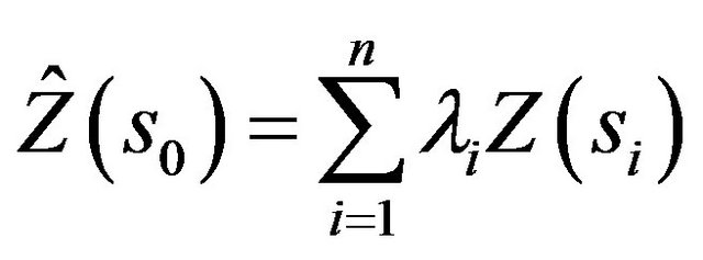
A type of deterministic method widely applied in spatial modelling. The estimation is based upon weighted averages, which are proportional to the inverse of the distance between the interpolated and measured points [24]. The general formula is expressed as:
 (1)
(1)
where 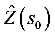 is the estimate value of Z in
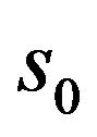 ,
, 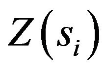 is the measure value locate in
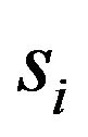 ,
, 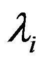 is the weight of
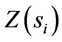 , n is the number of measurements used for estimate. And the weights are calculated as following:
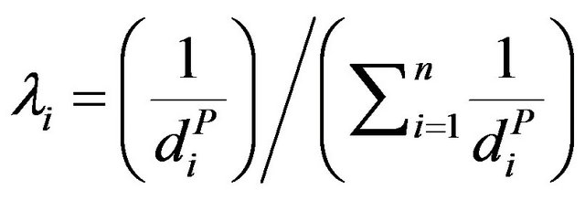 (2)
(2)
where di is the distance between x0 and xi, P is a power parameter, and n represents the number of sampled points used for the estimation. The main factor affecting the accuracy of IDW is the value of the power parameter. As the distance increases weights diminish, especially when the value of the power parameter increases. Nearby stations have a heavier weight and, therefore, more influence on the estimation [8,13,25]. After many trials, the best validated power parameter gotten was 1.5.
3.2. Spline Tension (Spline)
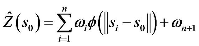
Spline is classified as a deterministic method and belongs to the radial basis functions (RBF) group. RBF encloses a series of exact interpolation techniques, where the spatial predictions must go through each measured sample value [8]. The predictor is a linear combination of functions,
 (3)
(3)
where 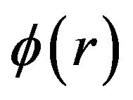 is a radial basis function (see Formula 4),
  is Euclidean distance between the prediction location s0 and each data location si, and
 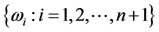 are weights to be estimated. As opposed to IDW, Spline methods can predict values above the maximum and below the minimum measured values. Spline is normally used for calculating smooth spatial distributions from a large number of data points. The technique may not be appropriate when there are large changes in observation values within a short horizontal distance [8,26]. In a previous task, all spline methods available in the Geostatistical Analyst tool of ArcGIS®9 were tested. From that, spline tension with smoothing parameter 2.0 × 10⁻⁴ revealed a slightly better performance than the other spline methods, and its function is described as:
 (4)
(4)
where σ is the smoothing parameter, K0(x) is the modified Bessel function, and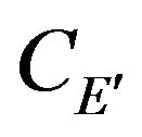 is the Euler constant [27].
3.3. Ordinary Kriging (OK)
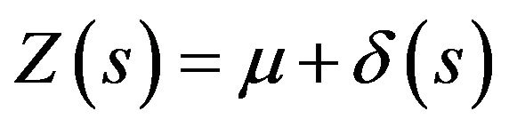
The kriging family, also known as Geoestatistics methods, is based on the idea that values measured at near locations tend to be more related than values measured at other locations [2]. Similar to IDW, kriging also uses a weighting, however as a probabilistic method, kriging depends on spatial and statistical relationships to predict unmeasured points [8]. Empirical semivariogram functions provide means for quantifying the spatial autocorrelation of datasets which is then included in the spatial model [28]. Kriging equation is based on spatial optimal linear prediction, where the unknown mean of the random process is estimated through the best linear unbiased estimator (B.L.U.E.). The estimator is “unbiased” because the mean of error is 0; “linear” since the estimated values are weighted linear combinations of the available data; and “best” because the estimator aims to minimize the variance of the errors [29]. For this work, the Ordinary Kriging performed the best validation among the other kriging methods. The prediction of Ordinary Kriging is a linear combination of measured values where the constant mean (μ) is assumed to be unknown [5,25,30]. The Ordinary Kriging representation for spatial stochastic process Z(s) is:
 (5)
(5)
where μ is unknown expected value of random process, δ(s) is a zero mean intrinsically stationary random process with existing semivariogram γ(H). The estimator 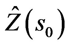 can be expressed as Formula (1). Linear coefficients
 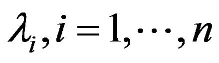 are calculated under the condition for uniformly unbiased predictor as:
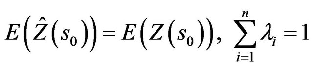 (6)
(6)
and under the restriction of minimal prediction error variance 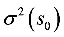 at location
 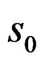 as:
as:
 (7)
(7)
Concerning to the empirical semivariogram model, the spherical semivariogram was applied due to its linear behavior at the origin [14]. The spherical model is one of the most commonly used models and it is written as:
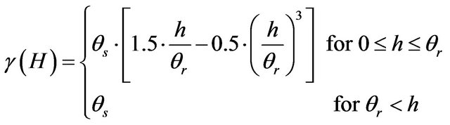 (8)
(8)
where θs is the sill value, H is the lag vector, and h is the length of H (distance between two points), θr is the range of the model.
3.4. CoKriging (CoOK)
CoKriging is an extension of kriging where more than one auxiliary variables can be added to the prediction. In a conventional kriging model, a response is assumed to be a spatial random process with stationary covariance function, what implies that the smoothness of a response is fairly uniform in each region of the domain area [31]. However, cases are common where the level of smoothness of a response could change considerably due to geophysical characteristics [32]. In such situations, cokriging is a regularly used technique where interpolations are improved by adding secondary attributes that may drive the spatial distribution of the variable in concern, for instance longitude, latitude and elevation [33]. Cokriging is most effective when the covariates are highly correlated [13]. In this case an isotopic cokriging, where data is available for each variable at all sampling points [5], was used. According to Cressie [30], a multivariate process can be written with the n x k matrix:
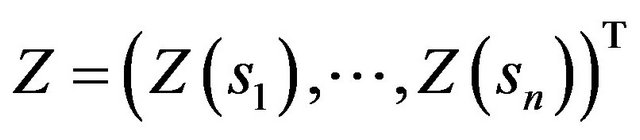 (9)
(9)
With i, j-th element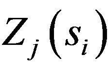 ,
, 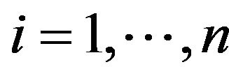 in
in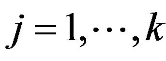 . Predicting the
 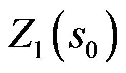 based on
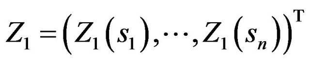 and on the covariables
 . The same assumptions as by ordinary kriging are expected for each of the k variables. The kriging predictor of
 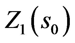 is a linear combination of all available data values of all k variables:
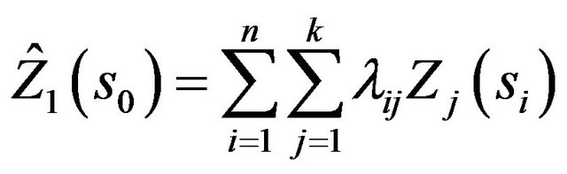 (10)
(10)
Assuming a uniformly unbiased predictor with the conditions:
 (11)
(11)
Therefore, the best linear unbiased predictor is obtained by minimizing
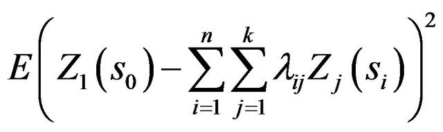 (12)
(12)
In this study, the spherical semivariogram was applied for all variables of interest.
3.5. Multiple Linear Regression (MReg)
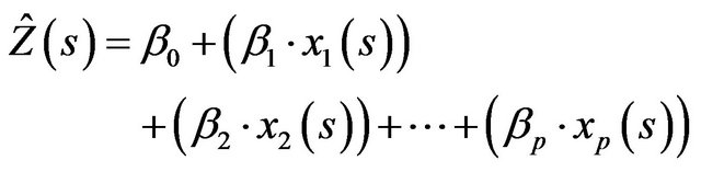
Multiple linear regression is a probabilistic method which expresses the relation between a predicted variable and explanatory variables. In a deterministic manner, it is assumed that the spatial distribution of rainfall is dependent on physical factors, for instance longitude, latitude and elevation. A limitation of the technique is the risk of predictions move into extrapolations due to its dependence on the fit of the regression model and distribution of the input datasets [34]. On the other hand, the simplicity of the multiple regression method can produce reasonable results and its analysis may significantly improve the GIS techniques for elaborating an objective mapping [19,20,35-37]. In its simplest form it is used to fit a straight line through points scattered in a plane. The mathematical background is described as:
 (13)
(13)
where 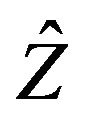 is the predicted variable at location s;
 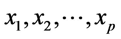 are explanatory variables at the concerning point; and β0 is the intercept and
 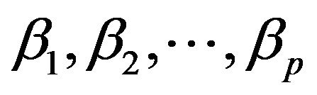 are coefficients of linear combination.
3.6. Residual Interpolation (MRegIDW)
The residual interpolation is classified as a combined method where both probabilistic and deterministic methods are applied. The residuals of a multiple linear regression model are calculated for each sample location and interpolated using a deterministic method, in this case IDW [2,13,22]. In other words, the first-order trend component (i.e., multiple regression model) is removed from the observations before a spatial interpolation technique is applied. The resulting gridded estimates are then added to the gridded multiple linear regression model [21]. The simplicity, robustness and accuracy of the residual interpolation method using multiple linear regression with IDW of the residuals was confirmed and suggested by Nalder and Wein [13]. The basic formula is defined as:
 (14)
(14)
where 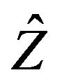 is the predicted variable at location s, as demonstrated in formula Equation (13); and
 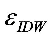 is the result of the interpolated residuals at location
  using IDW.
3.7. Calculation and Validation
All calculations were performed using the Geostatistical Analyst tool of ArcGIS®9. Multiple linear regression equations were calculated with a standard statistical program and computed by using map calculator functions in ArcGIS®9.
Moreover, in order to achieve a robust model with a realistic complexity, geophysical data was rescaled to 1000 × 1000 m grid resolution. Before producing spatial distribution maps, the accuracy of estimations must be assessed. Cross-validation and validation may assist the decision to which model provides the best predictions [2]. The calculated statistics provides a diagnostics whether the model and/or its associated parameter values are reasonable [8]. Cross-validation is probably the most widely applied method within climatology. In a cross-validation technique, one data point is left out of the data sample at a time while all the other data points are used to estimate the value for the concerning point left. This procedure is repeated until a value is estimated for all original data points [25].
One objection to using cross validation is that the whole data sample often is used to define the interpolation model, and that the validation therefore might be considered not to be totally independent [2]. In order to suppress problems of using cross-validation an independent validation procedure described by statistics, based on the absolute values of observed and estimated elements is applied. The procedure consists in splitting the data sample into two parts. Hence, 51 stations were used for interpolation purposes, while the remaining 9 stations were used for independent validation (Figure 1).
Four approaches were used for the comparison:
1) Visual analysis according to technical plausibility of prediction distribution;
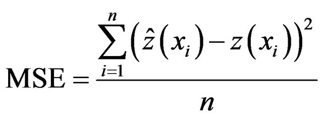
2) Mean square error (MSE) measures the difference between observed (z) and modeled 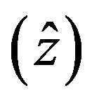 in its average of the squares. This error is usually used as a criterion to compare the results of interpolation methods and should be as low as possible [2];
 (15)
(15)
3) Correlation coefficient (r), also referred to as Pearson’s coefficient, is a measure of the linear dependence between two variables, in this case, the observed (z) and modeled 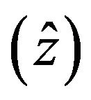 [2];
[2];
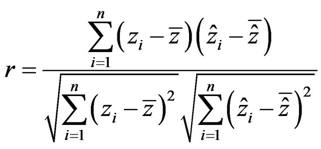 (16)
(16)
4) Nash-Sutcliffe efficiency criterion (NS). Although widely applied for validating hydrological models, the Nash-Sutcliffe efficiency criterion can also be applied to assess the performance of interpolation methods in climatology [38]. This approach takes the real quantities more into account than the correlation coefficient and therefore might be appropriated for the validation of rainfall.
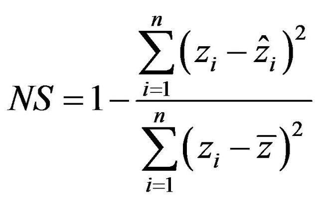 (17)
(17)
Nevertheless, no matter which interpolation technique is used, the interpolation values are only estimates of what the real values should be at a particular location. Therefore, for any analysis of interpolated observed data, the degree of uncertainty must be considered [17,39].
4. Results
Following the visual analysis, all methods have shown similar pattern on the spatial distribution of rainfall. Figure 2 illustrates the heterogenic distribution of rainfall where more accentuated amounts are observed over the North-West and West parts of the model region. However IDW, Spline, OK and CoOK do not capture local variations as the multiple regression models do. Since MReg and MRegIDW take into account physiographic elements, their maps illustrate more fine details, especially in the last case where residuals where included. Moreover, spatial and temporal distribution of precipitation can be explained by its dependence on the Amazonian atmospheric circulation system, located in Northwest from the study region. Intensive rainfall over central
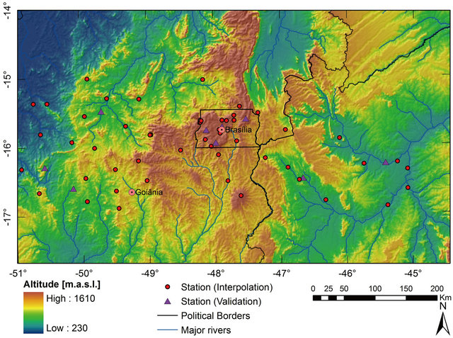
Figure 1. Distribution of the station network and topography of the model area (Central Brazil).
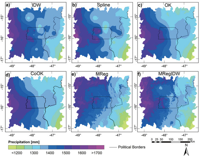
Figure 2. Annual precipitation (1971-2000) maps of Distrito Federal and surroundings (delimitated by watershed) using different interpolation methods. (e) and (f) at 1000 × 1000 m grid resolution.
Brazil, which occurs between December and February, is carried from the Equatorial Atlantic region by low level east winds when deviated from north-west toward southeast due to the Andes barrier [15,40,41]. At the same period it is observed a band of cloudiness and moisture which extends over Amazon region to the Subtropical Atlantic Ocean with orientation northeast-southwest denominated South Atlantic Convergence Zone-SACZ [42]. Topography also plays a significant role on rainfall mechanisms by forcing the air lift in higher areas, as in west of the Distrito Federal, creating greater convective activity compared to areas downwind of these natural highs [15]. Following the literature, the multiple regression model (MReg), using geographical position and altitude as explanatory variables, has performed very reliable results showing fairly the same distribution patterns as univariate methods. Figure 3 clearly shows the dependence of precipitation on geographical position and altitude. Results supports the inclusion of physiographic variables in the spatial interpolation approach, where the variance of multiple linear regression model was explained of about 77% for annual precipitations, 68% for summer (DJF), 81% for autumn (MAM), 44% for winter (JJA) and 69% for spring (SON). As the residual interpolation (MRegIDW) comprises both multivariate probabilistic method and univariate deterministic method, visual analysis confirms its higher performance than others.
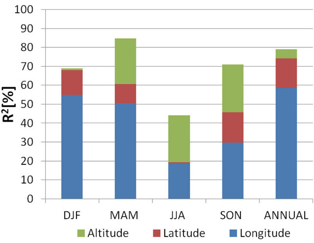
Figure 3. Description of the explanatory role of each significant physiographical parameter in the stepwise regression of seasonal and annual precipitation (1971-2000).
Tables 1 and 2 show the mean square error and correlation coefficient between measured and estimated values, respectively. Spatial interpolation for summer (DJF) rainfall has the lowest error and highest correlations when IDW method is applied. While in autumn (MAM) all methods, out of Spline demonstrated low errors/high correlation. In the other hand, MReg has the highest error and lowest correlation in summer. In winter (JJA), the OK and CoOK methods have the lowest errors/highest correlation, while MRegIDW the opposite. However, the rainfall average in this season is very low (ca. 26 mm) and therefore statistical validation measures for this season might not drive the choice or exclusion of an interpolation method. In spring (SON) the OK, IDW and MRegIDW have the lowest error/highest correlation, while MReg the highest error/lowest correlation. Inversely from Spline, the MRegIDW method has demonstrated the best results when annual rainfall is interpolated. Moreover, Table 3 exhibits the results according to the Nash-Sutcliffe method where IDW, followed by OK, CoOK and MRegIDW have performed the best predictions.
Raster statistics of annual precipitation shows that the difference between estimations methods is low, where the highest and lowest averages are 1428.8 mm (IDW) and 1404.2 mm (OK), respectively. Moreover the uncertainty, which is a function of observation density, must be taken into account. The representativity of the observation network is a very challenging issue within climatology [43]. Networks usually have an irregular spatial distribution, and are mostly located in populated areas and lower altitudes [2]. Among others (e.g., Thiessen polygons), the representativity of observations can be described by standard error maps, for instance from ordinary kriging methods. Figure 4 illustrates quite clearly the problems that arise with an irregular observation network. Low uncertainties are located especially in the Distrito Federal domain area and populated areas in Goiás state, for instance in the capital Goiânia and surroundings. Remote areas in north and north-east, where most of the observations are available just from the eighties due to the fact that these areas have been later occupied, are
Table 1. Mean square error (mm) between measured and predicted values. Underlined-Highest errors; Italic-Lowest errors.
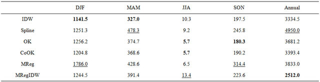
Table 2. Correlation coefficient between measured and predicted values. Underlined-Lowest correlation; Italic-Highest correlation.
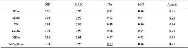
Table 3. Nash-Sutcliffe criterion between measured and predicted values. Underlined-Lowest value; Italic-Highest value.
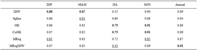
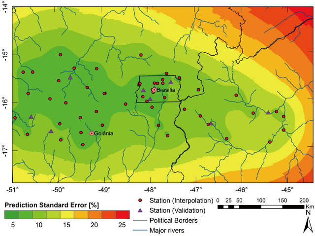
Figure 4. Uncertainties of interpolation demonstrated by prediction standard error [%] map of Ordinary Kriging for annual accumulated precipitation in Central Brazil.
under the influence of high uncertainties.
5. Conclusion
Deterministic, probabilistic and combined techniques were compared for the interpolation of seasonal and annual precipitation climatology (1971-2000) in Distrito Federal and surroundings. The dependence of long-term accumulated rainfall on local physiography was investigated. According to literature, regional precipitation patterns are very likely dependent on atmospheric circulation patterns originated from Amazon region and might be increased due to orography. In order to assess the performance of the methods tested, a validation approach based on visual analysis and basic statistics was applied. Concerning to visual analysis, the multiple linear regression models have shown finer details than others. The comparative study demonstrates that most interpolation methods give similar results wherever observation network is dense. However, including geographical variables in the estimation provides more detailed maps. Additionally, the addition of residuals interpolation generates more reliable predictions with low errors for annual precipitation and most of the seasons. MSE, correlation coefficient and Nash-Sutcliffe criterion confirmed the trustworthy prediction of IDW, OK and residual interpolation (MRegIDW), although the remaining methods also performed realistic results. Moreover, the multiple linear regression technique, using geographical position and altitude as explained variables, proved the dependence of accumulated rainfall on geophysical factors. Uncertainties on random and systematic errors of observations have been minimized by applying detection of suspicious values and homogenization tests, respectively. Furthermore, interpolation uncertainties, which are dependent on the representativity of observation network, were reduced by the high observation density in Distrito Federal as well as by the expansion of the model area from ca. 5.800 km2 (Distrito Federal and surroundings) to ca. 332.000 km2 (Central Brazil), where more stations are available. However, spatial representation of precipitation over north-east of Distrito Federal and surroundings, must be carefully interpreted due to the high uncertainties of the interpolation methods. Further research should investigate whether other environmental descriptors, such as water reservoirs or the slope orientation, allow one to explain a larger proportion of the spatial variability displayed by rainfall, especially in the dry season (JJA). Moreover, in order to validate the performance of the MRegIDW method for other periods where observation network is higher, maps should be generated using the same stations applied in this study against datasets with more available stations, for instance the 1981-2010 climatological period.
6. Acknowledgements
The author wishes to thank the International Water Research Alliance Saxony-IWAS initiative and the International Postgraduate Studies in Water Technologies-IPSWaT scholarship program (both funded by the German Federal Ministry of Education and Research, BMBF) for the opportunity given.
REFERENCES
- M. Strauch, Ch. Bernhofer, S. Koide, M. Volk, C. Lorz and F. Makeschin, “Using Precipitation Data Ensemble for Uncertainty Analysis in SWAT Streamflow Simulation,” Journal of Hydrology, Vol. 414-415, 2012, pp. 413- 424.
- O. Tveito, M. Wegehenkel, F. van der Wel and H. Dobesch, “The Use of Geographic Information Systems in Climatology and Meteorology: COST 719,” Luxemburg: COST Action719, 2008.
- A. Perdigao, “GIS, Climatology and Meteorology,” In: H. Dobesch, P. Dumolard and I. Dyras, Eds., Spatial Interpolation for Climate Data: The Use of GIS in Climatology and Meteorology, ISTE, London, 2010, pp. 3-24.
- S. Baillargeon, “Kriging Review of the Theory and Application to the Interpolation of Precipitation Data,” M.Sc. Thesis, University of Laval, Quebec, 2005.
- H. Wackernagel, “Multivariate Geostatistics,” Springer, Berlin, 2003.
- F. Renard and J. Comby, “Evaluation of Rainfall Spatial Interpolation Methods in Urban Area for a Better. Management of Extreme Rainy Events: The Case of the Urban Area of Greater Lyon,” La houile Blanche, No. 6, 2006, pp. 75-78.
- D. Courault and P. Monestiez, “Spatial Interpolation of Air Temperature According to Atmospheric Circulation Patterns in Southeast France,” International Journal of Climatology, Vol. 19, No. 4, 1999, pp. 365-378.
- K. Johnston, J. M. Ver Hoef, K. Krivoruchko and N. Lucas, “Using ArcGIS Geostatistical Analyst,” ESRI, Redlands, 2001.
- C. Lorz, G. Abbt-Braun, F. Bakker, P. Borges, H. Börnick, L. Fortes, F. Frimmel, A. Gaffron, N. Hebben, R. Höfer, F. Makeschin, K. Neder, H. L. Roig, B. Steiniger, M. Strauch, D. H. Walde, H. Weiß, E. Worch and J. Wummel, “Challenges of an Integrated Water Resource Management for the Distrito Federal, Western Central Brazil: Climate, Land-Use and Water Resources,” Environmental Earth Sciences, Vol. 65, No. 5, 2012, pp. 1363-1366.
- W. J. Dixon, “Analysis of Extreme Values,” Annals of Mathematical Statistics, Vol. 21, No. 4, 1950, pp. 488-506.
- J. Franke, “Risiken des Klimawandels für den Wasserhaushalt—Variabilität und Trend des Zeitlichen Niederschlagsspektrums,” In: Ch. Bernhofer and V. Goldberg, Eds., Antje Tittebrand, Analysis of the Spatial Heterogeneity of Land Surface Parameters and Energy Flux Densities, Part 1, Johannes Franke, Risiken des Klimawandels für den Wasserhaushalt—Variabilität und Trend des Zeitlichen Niederschlagsspektrums, Part 2, Tharandter Klimaprotokolle, Vol. 15, 2009.
- METI/NASA, “Advanced Spaceborne Thermal Emission and Reflection Radiometer-ASTER Global Digital Elevation Model,” Ministry of Economy, Trade and Industry of Japan (METI) and the National Aeronautics and Space Administration (NASA), 2009. http://asterweb.jpl.nasa.gov/gdem.asp
- I. A. Nalder and R. W. Wein, “Spatial Interpolation of Climatic Normals: Test of a New Method in the Canadian Boreal Forest,” Agriculture and Forest Meteorology, Vol. 92, No. 4, 1998, pp. 211-225.
- P. G. Goovaerts, “Geostatistical Approaches for Incorporating Elevation into the Spatial Interpolation of Rainfall,” Journal of Hydrology, Vol. 228, No. 1-2, 2000, pp. 113-129.
- C. Vera, W. Higgins, J. Amador, T. Ambrizzi, R. Garreaud, D. Gochis, D. Gutzler, D. Lettenmaier, J. Marengo, C. R. Mechoso, J. Nogues-Paegle, P. L. Silva Diaz and C. Zhang, “Towards a Unified View of the American Monsoon System,” Journal of Climate, Vol. 19, No. 20, 2006, pp. 4977-5000.
- L. M. Alves, “Clima da Região Centro-Oeste do Brasil,” In: I. F. A. Cavalcanti, N. J. Ferreira, M. G. A. J. Da Silva and M. A. F. Silva Dias, Tempo e Clima no Brasil, Oficina de Textos, São Paulo, 2009, pp. 235-241.
- T. Tao, B. Chocat, S. Liu and K. Xin, “Uncertainty Analysis of Interpolation Methods in Rainfall Spatial Distribution—A Case of Small Catchment in Lyon,” Journal of Water Resource and Protection, Vol. 1, No. 2, 2009, pp. 136-144.
- C. Daly, R. P. Neilson, D. L. Philips, “A Statistical-Topographical Model for Mapping Climatological Precipitation over Mountainous Terrain,” Journal of Applied Meteorology, Vol. 33, No. 2, 1994, pp. 140-158. doi:10.1175/JAMC-D-11-082.1
- S. Naoum and I. Tsanis, “Orographic Precipitation Modeling with Multiple Linear Regression,” Journal of Hydrologic Engineering, Vol. 9, No. 2, 2004, pp. 79-102.
- A. Mair and A. Fares, “Comparison of Rainfall Interpolation Methods in a Mountainous Region of a Tropical Island,” Journal of Hydrologic Engineering, Vol. 16, No. 4, 2011, pp. 371-383.
- O. E. Tveito and E. J. Førland, “Mapping Temperatures in Norway Applying Terrain Information, Geostatistics and GIS,” Norsk Geografisk Tidsskrift—Norwegian Journal of Geography, Vol. 53, No. 4, 1999, pp. 202-212.
- R. Lhotellier, “Spatialisation des Températures en Zone de Montagne Alpine,” Ph.D. Dissertation, Université Joseph Fourier, Grenoble, 2005.
- C. Portalés, N. Boronat, J. E. Pardo-Pascual and A. Balaguer-Beser, “Seasonal Precipitation Interpolation at the Valencia Region with Multivariate Methods Using Geographic and Topographic Information,” International Journal of Climatolology, Vol. 30, No. 10, 2010, pp. 1547- 1563.
- D. Shepard, “A Two-Dimensional Interpolation Function for Irregularly-Spaced Data,” Proceedings of the 23rd Association for Computing Machinery Annual Conference, New York, 1968, pp. 517-524.
- E. H. Isaaks and R. M. Srivastava, “An Introduction to Applied Geostatistics,” Oxford University Press, New York, 1989.
- M. F. Hutchinson, “Interpolation of Rainfall Data with Thin Plate Smoothing Splines: I Two Dimensional Smoothing of Data with Short Range Correlation,” Journal of Geographic Information and Decision Analysis, Vol. 2, No. 2, 1998, pp. 139-151.
- M. Abramowitz and I. A. Stegun, “Handbook of Mathematical Functions,” Dover, New York, 1965
- P. G. Goovaerts, “Geostatistics for Natural Resources Evaluation,” Oxford University Press, New York, 1997.
- N. Cressie, “The Origins of Kriging,” Mathematical Geology, Vol. 22, No. 3, 1990, pp. 239-252.
- N. Cressie, “Statistics for Spatial Data,” Wiley, New York, 1991.
- C. J. Paciorek, “Nonstationary Gaussian Processes for Regression and Spatial Modelling,” Ph.D. Dissertation, Carnegie Mellon University, Pittsburgh, 2003.
- Y. Xiong, W. Chen, D. Apley and X. Ding, “A Nonstationary Covariance-Based Kriging Method for Metamodeling in Engineering Design,” International Journal for Numerical Methods in Engineering, Vol. 71, No. 6, 2007, pp. 733-756. doi:10.1002/nme.1969
- A. Stein, A. C. Van Eijnsbergen and L. G. Barendregt, “Cokriging Nonstationary Data,” Mathematical Geology, Vol. 23, No. 5, 1991, pp. 703-719. doi:10.1007/BF02082532
- A. D. Hartkamp, K. De Beurs, A. Stein and J. W. White, “Interpolation Techniques for Climate Variables,” NRGGIS Series 99-01, CIMMYT, Mexico, 1999.
- M. Ninyerola, X. Pons and J. M. Roure, “A Methodological Approach of Climatological Modelling of Air Temperature and Precipitation through GIS Techniques,” International Journal of Climatology, Vol. 20, No. 14, 2000, pp. 1823-1841. doi:10.1002/1097-0088(20001130)20:14<1823::AID-JOC566>3.0.CO;2-B
- K. Stahl, R. D. Moore, J. A. Floyer, M. G. Asplin and I. G. McKendry, “Comparison of Approaches for Spatial Interpolation of Daily Air Temperature in a Large Region with Complex Topographyand Highly Variable Station Density,” Agriculture and Forest Meteorology, Vol. 139, No. 3-4, 2006, pp. 224-236. doi:10.1016/j.agrformet.2006.07.004
- H. Chai, W. Cheng, C. Zhou, X. Chen, X. Ma and S. Zhao, ”Analysis and Comparison of Spatial Interpolation Methods for Temperature Data in Xinjiang Uygur Autonomous Region, China,” Natural Science, Vol. 3, No. 12, 2011, pp. 999-1010. doi:10.4236/ns.2011.312125
- J. E. Nash and J. V. Sutcliffe, “River Flow Forecasting through Conceptual Models part I—A Discussion of Principles,” Journal of Hydrology, Vol. 10, No. 39, 1970, pp. 282-290. doi:10.1016/0022-1694(70)90255-6
- J. P. Chiles and P. Delfiner, “Geostatistics. Modeling Spatial Uncertainty,” John Wiley & Sons, New York, 1999.
- H. Virji, “A Preliminary Study of Summertime Tropospheric Circulation Pattern over South America Estimated from Cloud Winds,” Monthly Weather Review, Vol. 109, No. 3, 1981, pp. 599-610. doi:10.1175/1520-0493(1981)109<0599:APSOST>2.0.CO;2
- M. A. Gan, V. E. Kousky and C. F. Ropelewski, “The South America Monsoon Circulation and Its Relationship to Rainfall over West-Central Brazil,” Journal of Climate, Vol. 17, No. 1, 2004, pp. 47-66. doi:10.1175/1520-0442(2004)017<0047:TSAMCA>2.0.CO;2
- L. M. V. Carvalho and C. Jones, “Zona de Convergência do Atlântico Sul,” In: I. F. A. Cavalcanti, N. J. Ferreira, M. G. A. J. Da Silva and M. A. F. Silva Dias, Eds., Tempoe Clima no Brasil, Oficina de Textos, São Paulo, 2009, pp. 95-109.
- A. Jansson, O. E. Tveito, P. Pirinen and M. Scharling, “NORDGRID-A Preliminary Investigation on the Potential for Creation of a Joint Nordic Gridded Climate Dataset,” met.no Report, No. 3, 2007. p. 48.