World Journal of Nano Science and Engineering
Vol.06 No.02(2016), Article ID:67550,20 pages
10.4236/wjnse.2016.62009
Fourth-Order Compact Formulation for the Resolution of Heat Transfer in Natural Convection of Water-Cu Nanofluid in a Square Cavity with a Sinusoidal Boundary Thermal Condition
Mostafa Zaydan, Naoufal Yadil, Zoubair Boulahia, Abderrahim Wakif, Rachid Sehaqui
Mechanical Laboratory, Faculty of Sciences, Hassan II University, Ain Chock Maarif, Casablanca, Morocco

Copyright © 2016 by authors and Scientific Research Publishing Inc.
This work is licensed under the Creative Commons Attribution International License (CC BY).
http://creativecommons.org/licenses/by/4.0/


Received 11 April 2016; accepted 18 June 2016; published 21 June 2016
ABSTRACT
In the present work, we numerically study the laminar natural convection of a nanofluid confined in a square cavity. The vertical walls are assumed to be insulated, non-conducting, and impermeable to mass transfer. The horizontal walls are differentially heated, and the low is maintained at hot condition (sinusoidal) when the high one is cold. The objective of this work is to develop a new height accurate method for solving heat transfer equations. The new method is a Fourth Order Compact (F.O.C). This work aims to show the interest of the method and understand the effect of the presence of nanofluids in closed square systems on the natural convection mechanism. The numerical simulations are performed for Prandtl number ( ), the Rayleigh numbers varying between
  and for different volume fractions
  varies between 0% and 10% for the nanofluid (water + Cu).
Keywords:
Nanofluid, Heat Transfer, Natural Convection, Fourth-Order Compact (F.O.C) Formulation, Numerical Performance, Sinusoidal Boundary Thermal Condition

1. Introduction
In a better description, nanofluids are engineered colloidal suspensions of nanoparticles (1 - 100 nm) in a base fluid. Common base fluids include water, oil, and Ethylene Glycol while nanoparticles are typically made of chemically stable metals, metal oxides or carbon in various forms. The use of particles of nanometer dimension was first continuously studied by a research group at the Argonne National Laboratory a decade ago. S. Choi [1] in 1995 was probably the first one who called the fluids with particles of nanometer dimensions “nanofluids”. He showed substantial augmentation of heat transported in suspensions of copper or aluminum nanoparticles in water and other liquids. Compared with suspended particles of millimeter or micrometer dimensions, nanofluids show better stability and rheological properties, dramatically higher thermal conductivities and no penalty in pressure drop. Several published literatures have mainly focused on the prediction and measurement techniques in order to evaluate the thermal conductivity of nanofluid. It is noticeable that only a few papers have discussed the convective heat transfer of nanofluids, including the experimental and theoretical investigation.
A numerical study of natural convection of copper-water nanofluide in a two dimensional enclosure was conducted by Khanafer et al. [2] . The nanofluid in the enclosure was assumed to be in single phase. It was found in any given Grashof number, heat transfer in the enclosure increased with the volumetric fraction of the copper nanoparticles in water. Lee et al. [3] measured the thermal conductivity of Al2O3 water and Cu-water nanofluids and indicated that the thermal conductivity of nanofluids increases with solid volume fraction. He concluded that any new models of nanofluide thermal conductivity should contain the effect of surface area and structure dependent behavior as well as the size effect. Xie et al. [4] added spherical and cylindrical shaped nano sized SiC particles to water and Ethylene Glycol, separately and found that cylindrical nanoparticles increased thermal conductivity more than spherical ones. The dependence of thermal conductivity of nanoparticles-fluid mixture was estimated by Xie et al. [5] . Some of the theoretical and experimental studies have been reported on convective heat transfer coefficient [6] - [9] .
Sandeep Naramgari and C. Sulochana [10] analyzed the momentum and heat transfer behavior of MHD nanofluid embedded with conducting dust particles past a stretching surface in the presence of volume fraction of dust particles. They solved equations numerically using Runge-Kutta based shooting technique and showed that the increase in the interaction between the fluid and particle phase enhanced the heat transfer rate and reduced the friction factor. Nader Ben-Cheikh et al. [11] studied natural convection in a square enclosure filled with a water based nanofluid (water with Ag, Cu, Al2O3 or TiO2 nanoparticles) with non-uniform (sinusoidal) temperature distribution maintained at the bottom wall. An accurate finite volume scheme along with a multi-grid technique is devised for the purpose of solution of the governing equations. Tiwari et al. [12] numerically investigated the behavior of copper-water nanofluid in a two sided lid-driven differentially heated cavity. They considered different cases characterized by the direction of movement of walls and found that both the Richardson number and direction of moving walls influenced the fluid flow and thermal behavior. Yadil et al. [13] study the Cu/Water nanofluids filled baffled square cavity.
The effects of Rayleigh number, volume fraction and partitions location on the average Nusselt number are studied. I.El Bouihi and R. Sehaqui [14] she simulate the flow features of nanofluids for a range of solid volume fraction χ and a sinusoidal thermal boundary condition, and we obtained correlations of heat transfer in enclosures for two different thermal boundary conditions on the left wall. Ami-Nossadati and Ghasemi [15] studied natural convection cooling of a localized heat source at the bottom of a nanofluid filled enclosure. Ogut [16] investigated natural convection of water-based nanofluids in an inclined enclosure with a heat source using the expression for calculating the effective thermal conductivity of solid-liquid mixtures proposed by Yu and Choi [17] . Ghasemi and Aminossadati [18] considered periodic natural convection in a nanofluid filled enclosure with oscillating heat flux. Non-uniform heating of surfaces in buoyancy driven flow in a cavity has significant effect of the flow and heat transfer characteristics and finds applications in various areas such as crystal growth in liquids, energy storage, geophysics, solar distillers and others. In a relatively recent study, Sarris et al. [19] reported that the sinusoidal wall temperature variation produced uniform melting of materials such as glass in their detailed study on the effect of sinusoidal top wall temperature variations in a natural convection within a square enclosure where the other walls are insulated. Corcione [20] studied natural convection in an air filled rectangular enclosure heated from below and cooled from above for a variety of thermal boundary conditions at the side walls. Roy and Basak [21] studied numerically natural convection flows in a square cavity with non-uniformly (sinusoidal) heated wall(s) using the finite element method. The bottom wall and one vertical wall were heated (uniformly and non-uniformly) and the top wall was insulated while the other vertical wall was cooled by means of a constant temperature bath. Sathiyamoorthy et al. [22] investigated steady natural convection flows in a square cavity with linearly heated side wall(s).
In order to optimize and improve heat transfer by natural convection in closed square cavity. Although extensive research has been given to cases of rectangular cavity filled nanofluid, few studies have focused on the study, theoretical or numerical discretizations high order (≥2). The numerical study of systems of equations in the heat transfer area is usually treated by various methods, sometimes numérical classics like Finite Elements (FE), Volume Finite (VF) and Finite Differences (DF). or using some software adapted as “FLUENT”. To solve fluid mechanics problems such as conductive heat transfer, convective or mixed into regular geometries.
More specific order four schemes have been used to solve the Navier-Stokes in enclosures without considering the energy equation by Ecran Erturk et C. Gokcol [2] . The objective of this work is to develop a new method for solving heat transfer equations in convection. The new method is a Fourth Order Compact. This work aims to show the interest of the method and understand the effect of the presence of nanofluids in closed square systems on the natural convection mechanism.
2. Mathematical Formulation
Consider a square cavity filled with a nanofluid. The vertical walls are assumed to be insulated, non-conducting, and impermeable to mass transfer. The horizontal walls are differentially heated, the low is maintained at hot condition (sinusoidal) when the high one is cold (Figure 1). The nanofluid in the enclosure is Newtonian, incompressible, and laminar. The nanoparticles are assumed to have a uniform shape and size. Moreover, it is assumed that both the fluid phase and nanoparticles are in thermal equilibrium state and they flow at the same velocity. The thermophysical properties of the nanofluid are assumed to be constant except for the density variation in the buoyancy force, which is based on the Boussinesq approximation.
We have considered the continuity, momentum and energy equations for a Newtonian, Fourier constant property fluid governing an unsteady, two-dimensional flow. It is further assumed that radiation heat transfer among sides is negligible with respect to other modes of heat transfer. Under the assumption of constant thermal properties, the Navier-Stokes equations for an unsteady, incompressible, two-dimensional flow are:
Continuity equation:
 (1)
(1)
x-momentum equation:

Figure 1. Physical model the coordinate system.
 (2)
(2)
y-momentum equation:
 (3)
(3)
Energy equation:
 (4)
(4)
where 
The viscosity of the nanofluid can be estimated with the existing relations for the two-phase mixture. The equation given by Brinkman [23] has been used as the relation for effective viscosity in this problem, as given by Xuan and Li [24] have experimentally measured the apparent viscosity of the transformer oil-water nanofluid and of the water-copper nanofluid in the temperature range of 20˚C - 50˚C. The experimental results reveal relatively good agreement with Brinkman’s theory. The thermophysical properties of fluid and the solid phases are shown in Table 1.
The effective density of the nanofluid at reference temperature is
 (5)
(5)
The heat capacitance of the nanofluid is expressed as Abu-Nada [25] and Khanafer et al. [2]
 (6)
(6)
The effective thermal conductivity of the nanofluid is approximated by the Maxwell-Garnetts model [26]
 (7)
(7)
Equations (1)-(4) can be converted to the dimensionless forms by definition of the following parameters as:


Hence, the governing equations of continuity, linear momentum and energy for unsteady laminar flow in Cartesian coordinates take the following dimensionless form:

Table 1. Thermophysical properties of water and nanoparticles.
 (8)
(8)
 (9)
(9)
 (10)
(10)
 (11)
(11)
The enclosure boundary conditions consist of no-slip and no penetration walls, U = V = 0 on all four walls. The thermal boundary conditions on the bottom wall is such that . The left and right vertical walls are assumed to be insulated, non-conducting, and impermeable to mass transfer
 and the bottom wall are at the cold temperature
The governing equations for the present study in  formulation taking into the account the above mentioned assumptions are written in dimensionless form as:
Kinematics equation:
 (12)
(12)
Vorticity equation:
 (13)
(13)
where: 
Energy equation:
 (14)
(14)
Before turning to the application of the method of fourth order in the equations governing our problem we will combine Equations (12) and (13) in a condensed form by introducing a dummy variable , which replace either the temperature
  is the vorticity
 .
.
 (15)
(15)
All these terms are listed in Table 2.
Dimensionless boundary conditions for  are:
are:
For:  and
and ,
, 
For:  and
and ,
, .
.
For vorcicite Störtkuh et al. [27] have presented an analytical asymptotic solution near the corners of cavity and using finite element bilinear shape functions they also have presented a singularity-removed boundary condition for vorticity at the corner points as well as at the wall points. For the boundary conditions, in both of the numerical methods described above we follow Störtkuh et al. [27] and use the following expression for calculating vorticity values at the wall.
Table 2. Presentation of the different terms of the transport equation.
 (16)
(16)
For corner points, we again follow Störtkuh et al. [27] and use the following expression for calculating the vorticity values:
 (17)
(17)
where V is the speed of the wall in our case which is equal to 0 for the four stationary walls.
In explicit notation, for the wall points shown in Figure 2(a), the vorticity is calculated as the following:
 (18)
(18)
Similarly, for the corner points also shown in Figure 2(b), the vorticity is calculated as the following:
 (19)
(19)
The reader is referred to Störtkuh et al. [27] for details on the boundary conditions.
The local and averaged heat transfer rates at the bottom hot wall of the cavity are presented by means of the local and averaged Nusselt numbers, Nu and , which are, respectively determined as follows:
 (20)
(20)
 (21)
(21)
3. Method of the Fourth Order Compact
3.1. Introduction
High-Order Compact (HOC) formulations are becoming more popular in computational fluid dynamics (CFD) field of study. Compact formulations provide more accurate solutions in a compact stencil. In finite differences, a standard three-point discretization provides second-order spatial accuracy and this type of discretization is very widely used. When a high-order spatial discretization is desired, i.e. fourth-order accuracy, then a five- point discretization has to be used. However, in a five point discretization there is a complexity in handling the points near the boundaries. High-order compact schemes provide fourth-order spatial accuracy in a 3 × 3 stencil
 (a) (b)
Figure 2. Grid points at the wall and at the corner: (a) wall points and (b) corner points.
and this type of compact formulations does not have the complexity near the boundaries that a standard wide (five- point) fourth-order formulation would have. Dennis and Hudson [28] , MacKinnon and Johnson [29] , Gupta et al. [30] , Spotz and Carey [31] , Li et al. [32] , have demonstrated the efficiency of the HOC schemes on the stream function and vorticity formulation of two dimensions. In the literature, it is possible to find numerous different types of iterative numerical methods for the momentum equations. These numerical methods, however, could not be easily used in HOC schemes because of the final form of the HOC formulations used in References [28] - [32] . This fact might be counted as a disadvantage of HOC formulations that the coding stage is rather complex due to the resulting stencil used in these studies. It would be very useful if any numerical method for the solution of momentum equations described in books and papers could be easily applied to HOC formulations. E. Erturk and C. Gokcol [33] present a new Fourth-Order Compact Formulation. The difference of this formulation with References [28] - [32] is not in the way that the Fourth-Order Compact scheme is obtained. The main difference, however, is in the way that the final forms of the equations are written. The main advantage of this formulation is that, any iterative numerical method used for Navier-Stokes equations, can be easily applied to this new FOC formulation, since the final form of the presented FOC formulation is in the same form with the Navier?Stokes equations. Moreover, if someone already has a second-order accurate  code for the solution of conservation equations the mass and momentum, they can easily convert their existing code to fourth- order accuracy
  by just adding some coefficients into their existing code. In this study, we will applied Using this new compact formulation, we have solved the conservation equations of mass, momentum and energy in square cavity at the Rayleigh number varies in the range
  and for different solide volume fractions
  of nanoparticles (Cu) is varied as
 , taking water as a base fluid with a Prandtl number equal to
  using a very fine grid mesh to demonstrate the efficiency of this new formulation.
3.2. Principle Method of Fourth Order Compact
We will use the equations of streamlines , vorticity
  and energy
  dimensionless forms are given as follows:
Stream function:
 (22)
(22)
General equation of conservation:
 (23)
(23)
For first and second-order derivatives the following discretizations are fourth-order accurate:
 (24)
(24)
 (25)
(25)
where  and
and  are standard second-order central discretizations such that
 (26)
(26)
 (27)
(27)
If we apply the discretizations in Equations (24) and (25) to Equations (22) and (23), we obtain the following equation
 (28)
(28)
 (29)
(29)
In these equations we have third and fourth derivatives  of stream function and general equation of conservation bringing together the equations of vorticity and energy. In order to find an expression for these derivatives we use Equations (22) and (23).
For example, when we take the first and second x-derivative of the stream function Equation (22) we obtain
 (30)
(30)
 (31)
(31)
And also, by taking the first and second y-derivative of the stream function Equation (22) we obtain
 (32)
(32)
 (33)
(33)
Using standard second-order central discretizations given in Table 3, these equations can be written as
 (34)
(34)
 (35)
(35)
 (36)
(36)
 (37)
(37)
When we substitute Equations (35) and (37) into Equation (28) we obtain the following finite difference equation.
Table 3. Standard second-order central discretizations.
 (38)
(38)
We note that the solution of Equation (38) is also a solution to stream function Equation (22) with fourth-or- der spatial accuracy. Therefore, if we numerically solve Equation (38), the solution we obtain will satisfy the stream function equation up to fourth order accuracy.
In order to obtain a fourth-order approximation for the vorticity equation and energy (23), we follow the same procedure. When we take the first and second derivatives of the general equation of conservation (23) with respect to x- and y-coordinates we obtain:
 (39)
(39)
 (40)
(40)
 (41)
(41)
 (42)
(42)
If we substitute Equations (39) and (41) for the third derivatives of the general equation of conservation and into Equations (29), (40) and (42) and also if we substitute Equations (34) and (36), for the third derivatives of stream function into Equations (29), (40) and (42) and finally, if we substitute Equations (40) and (42) for the fourth derivatives of the general equation of conservation into Equation (29), then we obtain the following:
 (43)
(43)
where:

and 
Again we note that the solution of Equation (43) satisfy the vorticity and energy Equation (23) with fourth- order accuracy.
As the final form of our FOC scheme, we prefer to write Equations (38) and (43) as
 (44)
(44)
 (45)
(45)
where


 (46)
(46)
We note that the finite difference Equations (44) and (45) are fourth-order accurate  approximation of the stream function, vorticity and energy Equations (22) and (23). In Equations (44) and (45), however, if A, B, C, D, E and F are chosen to be equal to 0 then the finite difference Equations (44) and (45) simply become
 (47)
(47)
 (48)
(48)
Equations (47) and (48) are the standard second-order accurate  approximation of the stream-
function and the general equation of conservation (22) and (23). When we use Equations (44) and (45) for the numerical solution of the stream function and general equation of conservation, we can easily switch between second and fourth-order accuracy just by using homogeneous values for the coefficients A, B, C, D, E and F or by using the expressions defined in Equation (46) in the code.
We note that the numerical solutions of Equations (44) and (45), strictly provided that second-order discretizations in Table 3 are used and also strictly provided that a uniform grid mesh with and is used, are fourth-order accurate to streamfunction and the general equation of conservation (21) and (22). The only difference between Equations (44) and (45) and Equations (22) and (23) are the coefficients A, B, C, D, E and F. So these equations are of the same form, therefore, all the iterative numerical methods (such as SOR, ADI, factorization schemes, pseudo time iterations, etc.) used to solve stream-function, vorticity and energy Equations (22) and (23) can also be easily applied to fourth-order Equations (44) and (45). In our work we apply the ADI method on the equations of 4th order.
As a measure of convergence to the steady state, during the iterations we monitored three residual parameters. The first residual parameter, RES1, is defined as the maximum absolute residual of the finite difference equations of steady stream function and general Equations (44) and (45). These are, respectively, given as
 (49)
(49)
 (50)
(50)
The magnitude of RES1 is an indication of the degree to which the solution has converged to steady state. In the limit RES1 would be zero. The second residual parameter, RES2, is defined as the maximum absolute difference between two iteration steps in the stream function, vorticity and energy variables. These are, respectively, given as
 (51)
(51)
 (52)
(52)
RES2 gives an indication of the significant digit on which the code is iterating. The third residual parameter, RES3, is similar to RES2, except that it is normalized by the representative value at the previous time step. This then provides an indication of the maximum percent change in  and
and  in each iteration step. RES3 is defined as
 (53)
(53)
 (54)
(54)
In our calculations, for all Rayleigh numbers we considered that convergence was achieved when both  and
and  were achieved. Such a low value was chosen to ensure the accuracy of the solution. At these convergence levels, the second residual parameters were in the order of
  and
and , which means that the stream function, vorticity and energy variables are accurate to the 10th and 9th digit accuracy, respectively, at a grid point and even more accurate at the rest of the grids. In addition, at these convergence levels the third residual parameters were in the order of
  and
and , which means that the stream function, vorticity and energy variables are changing with 10% - 9% and 10% - 8% of their values, respectively, in an iteration step at a grid point and even with less percentage at the rest of the grids. These very low residuals ensure that our solutions are indeed very accurate.
4. Results and Discussion
In the present grid independence test, the Prandtl number is set to Pr = 6.2 (pure water). The nanoparticles are chosen to be copper (Cu) with a solid volume fraction  and a Rayleigh number Ra = 105. Numerical computations have been carried on five different grid sizes 32 × 32, 42 × 42, 62 × 62, 82 × 82 and 102 × 102 grid sizes. Table 4 regroups the values of the averaged Nusselt number through the hot wall and the maximum value of the stream function. Uniform grid has been used for all the computations. The distribution of the u-velocity in the vertical mid-plane and v-velocity in the horizontal mid-plane are shown in Figure 3. It is observed that the curves overlap with each other for 82 × 82 and 102 × 102. So a grid number of 82 × 82 is chosen for further computation.
Our code has been tested for natural convection fluid flows in differentially heated cavities and in Rayleigh- Bénard configuration for Rayleigh numbers between 103 and 106 (Table 5) and gave excellent results (see ref. [12] [14] [34] - [36] ).


Figure 3. Velocity profiles at mid-sections of the cavity for various meshes sizes (Ra = 105 and χ = 0.1).
Table 4. Grid independency results for water-Cu,  and
and .
.
Table 5. Comparaison between the present work and other studies for .
.
In this section, the nanofluid-filled enclosure is studied for a range of solid volume fraction  and the Rayleigh number varies from 103 to 105. For all simulations the considered base fluid is water (Pr = 6.2). In Figure 4, we present the streamlines (top) and isotherms (bottom) for 103 ≤ Ra ≤ 105, for the case of a water- Cu nanofluid and pure water. The value of solid volume fraction is set to
 . Figure 5 represents the same physical quantities but for a volume fraction value of
 . Due to the temperature distribution imposed at the bottom wall and to the boundary conditions on vertical walls, we observe a symmetry behavior in both the streamlines and in the contour maps of the isotherms. We can see that whatever the Rayleigh number and value of solid volume fraction, the flow is mainly composed of two counter-rotating circulating cells.
Figure 6 presents the velocity profiles V(X) and U(Y) along the mid-section of the enclosure X = 0.5 and Y = 0.5 for different values of χ and is in good concordance with the fact that the nanofluid moves slower than a pure water. Indeed, for Ra = 103, the deviation (relative to χ = 0) between the maximum values of vertical velocity is  for χ = 4% and
  for χ = 10%. By increasing the Rayleigh number, these deviations decrease. For Ra = 5 × 10⁴ and Ra = 105 these deviations are
 ,
,  ,
,  and
and  respectively. As far as the temperature distribution is concerned, clear differences are observed in the isotherm contour plots compared to the case χ = 0. These differences are accentuated as the solid volume fraction increases. These differences mean that the presence of nanoparticles affect especially the heat transfer rate through the enclosure.
The heat transfer distribution through the hot wall is displayed in Figure 7 through the plotted lines of the local Nusselt number for different values of Ra. One can see that for all combinations of Ra and χ, the local Nusselt number behavior is symmetric with respect to the plane X = 0.5. For low Rayleigh numbers, (Ra = 5 × 10³) and χ = 0, the transfer of heat through the hot wall is relatively low with a slight curvature at X = 0.5. This curvature is due to relatively higher intensity of the counter rotating cells represented by the highest value of  when χ = 0. When χ increases to χ = 0.1, the curvature at the center disappears because the fluid velocity decreases. The heat transfer in this case is maximum at X = 0.5 and is higher due to the presence of nanoparticles whose thermal conductivity is much greater than that of water. The same phenomena are observed almost on the curves related to Ra = 5 × 10⁴ and Ra = 5 × 10⁵ with a maximum heat transfer in the vicinity of X = 0.25 and X = 0.75. For example, for Ra = 5 × 10⁴, the maximum Nusselt number value is Numax = 7.374 and is situated at both locations X = 0.317 and X = 0.682 for χ = 0. For χ = 0.1, Numax = 10.394 and is located at X = 0.317 and X = 0.695.
The variations of average Nusselt number (Nu) with Ra and χ are shown in Table 6. For Ra = 103, there is a substantial increase in Nu as χ is increased above 2%. In general, Nu increases with χ. When χ is 2%, the increase is approximately 9.75%. When χ is 4%, the increase is approximately 19.51%. When χ is 8%, the increase is above 42.07%. For Ra = 104, as χ is increased to 2%, an increase of 6.03% is observed. A heat transfer augmentation of above 27.63% is obtained for  compared to
  or more is observed for different Rayleigh number Ra. Thus, one can conclude that the Nusselt number increases with the increase of the volume fraction χ and Rayleigh number Ra.
5. Conclusions
In this study the heat transfer enhancement in a two dimensional enclosure filled with nanofluids is studied
Figure 4. Streamlines and isotherms for the enclosure filled with water-Cu nanofluid (- - -),  and pure water (―) at different Rayleigh numbers.
Figure 4. Streamlines and isotherms for the enclosure filled with water-Cu nanofluid (- - -), and pure water (―) at different Rayleigh numbers.
Figure 5. Streamlines and isotherms for the enclosure filled with water-Cu nanofluid (- - -),  and pure water (―) at different Rayleigh numbers.
Figure 5. Streamlines and isotherms for the enclosure filled with water-Cu nanofluid (- - -), and pure water (―) at different Rayleigh numbers.


Figure 6. Velocity profiles along the mid-plane for different Ra and different solid volume fractions (Water-Cu).
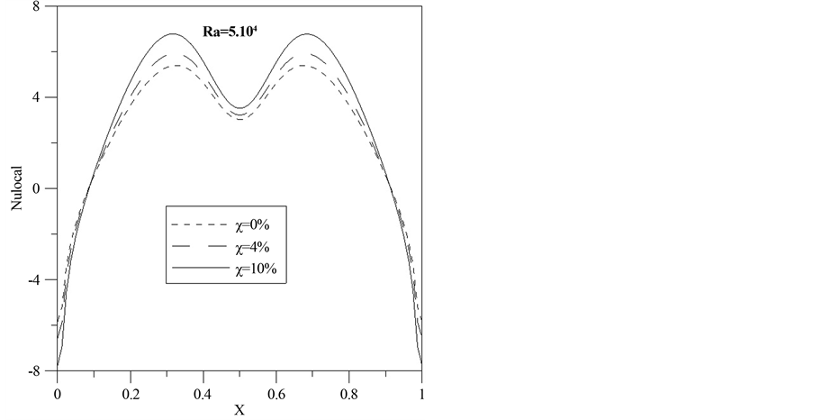


Figure 7. Local Nusselt number through the heated wall for different Ra and solid volume fractions (water-Cu).
Table 6. Comparison of average Nusselt number  for different Rayleigh number and various solid volume fractions.
numerically. This study presented a new fourth-order compact formulation and investigated the effect of a sinusoidal thermal boundary condition, for different Rayleigh number Ra and volume fractions of nanoparticles. The flow and temperature fields are symmetric near the middle plane of the enclosure due to the imposed symmetry condition on the bottom wall boundary. From the results of this work, the following main conclusions may be drawn:
・ The fourth-order accurate compact formulation was developed and was in agree with previous studies.
・ Our numerical code has been validated for different Rayleigh number.
・ A comparative study illustrates that the suspended nanoparticles substantially increase the heat transfer rate with an increase in the nanoparticles volume fraction for different Rayleigh number Ra Rayleigh number. Moreover, the nanofluid flows as well as the cooper nanoparticles increase.
In the near future, this study will be extended for different geometry studies and other types of base fluids and nanoparticles.
Cite this paper
Mostafa Zaydan,Naoufal Yadil,Zoubair Boulahia,Abderrahim Wakif,Rachid Sehaqui, (2016) Fourth-Order Compact Formulation for the Resolution of Heat Transfer in Natural Convection of Water-Cu Nanofluid in a Square Cavity with a Sinusoidal Boundary Thermal Condition. World Journal of Nano Science and Engineering,06,70-89. doi: 10.4236/wjnse.2016.62009
References
- 1. Choi, S. (1995) Enhancing Thermal Conductivity of Fluids with Nanoparticles. In: Siginer, D.A. and Wang, H.P., Eds., De-velopments and Applications of Non-Newtonian Flows, FED-Vol. 231/MD-Vol. 66, ASME, New York, 99-105.
- 2. Khanafer, K., Vafai, K. and Lightstone, M. (2003) Buoyancy-Driven Heat Transfer Enhancement in a Two-Dimensional Enclosure Utilizing Nanofluids. International Journal of Heat and Mass Transfer, 46, 3639-3653.
http://dx.doi.org/10.1016/S0017-9310(03)00156-X - 3. Lee, S., Choi, S.U.-S., Li, S. and Eastman, J. (1999) Measuring Thermal Conductivity of Fluids Containing Oxide Nanoparticles. Journal of Heat Transfer, 121, 280-289.
http://dx.doi.org/10.1115/1.2825978 - 4. Xie, H., Wang, J., Xi, T. and Liu, Y. (2002) Thermal Conductivity of Suspensions Containing Nanosized SiC Particles. International Journal of Thermophysics, 23, 571-580.
http://dx.doi.org/10.1023/A:1015121805842 - 5. Xie, H., Wang, J., Xi, T., Liu, Y. and Ai, F. (2002) Dependence of the Thermal Conductivity of Nanoparticle-Fluid Mixture on the Base Fluid. Journal of Materials Science Letters, 21, 1469-1471.
http://dx.doi.org/10.1023/A:1020060324472 - 6. Hwang, K.S., Jang, S.P. and Choi, S.U. (2009) Flow and Convective Heat Transfer Characteristics of Water-Based Al2O3 Nanofluids in Fully Developed Laminar Flow Regime. International Journal of Heat and Mass Transfer, 52, 193-199.
http://dx.doi.org/10.1016/j.ijheatmasstransfer.2008.06.032 - 7. Wen, D. and Ding, Y. (2004) Experimental Investigation into Convective Heat Transfer of Nanofluids at the Entrance Region under Laminar Flow Conditions. International Journal of Heat and Mass Transfer, 47, 5181-5188.
http://dx.doi.org/10.1016/j.ijheatmasstransfer.2004.07.012 - 8. Xuan, Y. and Li, Q. (2003) Investigation on Convective Heat Transfer and Flow Features of Nanofluids. Journal of Heat Transfer, 125, 151-155.
http://dx.doi.org/10.1115/1.1532008 - 9. Xuan, Y. and Li, Q. (2000) Heat Transfer Enhancement of Nanofluids. International Journal of Heat and Fluid Flow, 21, 58-64.
http://dx.doi.org/10.1016/S0142-727X(99)00067-3 - 10. Naramgari, S. and Sulochana, C. (2015) MHD Flow of Dusty Nanofluid over a Stretching Surface with Volume Fraction of Dust Particles. Ain Shams Engineering Journal, 7, 709-716.
http://dx.doi.org/10.1016/j.asej.2015.05.015 - 11. Ben-Cheikh, N., Chamkha, A.J., Ben-Beya, B. and Lili, T. (2013) Natural Convection of Water-Based Nanofluids in a Square Enclosure with Non-Uniform Heating of the Bottom Wall. Journal of Modern Physics, 4, 147-159.
http://dx.doi.org/10.4236/jmp.2013.42021 - 12. Tiwari, R.K. and Das, M.K. (2007) Heat Transfer Augmentation in a Two-Sided Lid-Driven Differentially Heated Square Cavity Utilizing Nanofluids. International Journal of Heat and Mass Transfer, 50, 2002-2018.
http://dx.doi.org/10.1016/j.ijheatmasstransfer.2006.09.034 - 13. Naoufal, Y., Zaydan, M. and Rachid, S. (2015) Numerical Study of Natural Convection in a Square Cavity with Partitions Utilizing Cu-Water Nanofluid. International Journal of Innovative Research in Science, Engineering and Technology, 4, 10354-10367.
- 14. El Bouihi, I. and Sehaqui, R. (2012) Numerical Study of Natural Convection in a Two-Dimensional Enclosure with a Sinusoidal Boundary Thermal Condition Utilizing Nanofluid. Engineering, 4, 445-452.
http://dx.doi.org/10.4236/eng.2012.48058 - 15. Aminossadati, S. and Ghasemi, B. (2009) Natural Convection Cooling of a Localised Heat Source at the Bottom of a Nanofluid-Filled Enclosure. European Journal of Mechanics-B/Fluids, 28, 630-640.
http://dx.doi.org/10.1016/j.euromechflu.2009.05.006 - 16. Ögüt, E.B. (2009) Natural Convection of Water-Based Nanofluids in an Inclined Enclosure with a Heat Source. International Journal of Thermal Sciences, 48, 2063-2073.
http://dx.doi.org/10.1016/j.ijthermalsci.2009.03.014 - 17. Yu, W. and Choi, S. (2003) The Role of Interfacial Layers in the Enhanced Thermal Conductivity of Nanofluids: A Renovated Maxwell Model. Journal of Nanoparticle Research, 5, 167-171.
http://dx.doi.org/10.1023/A:1024438603801 - 18. Ghasemi, B. and Aminossadati, S. (2010) Periodic Natural Convection in a Nanofluid-Filled Enclosure with Oscillating Heat Flux. International Journal of Thermal Sciences, 49, 1-9.
http://dx.doi.org/10.1016/j.ijthermalsci.2009.07.020 - 19. Sarris, I., Lekakis, I. and Vlachos, N. (2002) Natural Convection in a 2D Enclosure with Sinusoidal Upper Wall Temperature. Numerical Heat Transfer, Part A: Applications, 42, 513-530.
http://dx.doi.org/10.1080/10407780290059675 - 20. Corcione, M. (2003) Effects of the Thermal Boundary Conditions at the Sidewalls upon Natural Convection in Rectangular Enclosures Heated from Below and Cooled from Above. International Journal of Thermal Sciences, 42, 199-208.
http://dx.doi.org/10.1016/S1290-0729(02)00019-4 - 21. Roy, S. and Basak, T. (2005) Finite Element Analysis of Natural Convection Flows in a Square Cavity with Non-Uniformly Heated Wall(s). International Journal of Engineering Science, 43, 668-680.
http://dx.doi.org/10.1016/j.ijengsci.2005.01.002 - 22. Sathiyamoorthy, M., Basak, T., Roy, S. and Pop, I. (2007) Steady Natural Convection Flows in a Square Cavity with Linearly Heated Side Wall(s). International Journal of Heat and Mass Transfer, 50, 766-775.
http://dx.doi.org/10.1016/j.ijheatmasstransfer.2006.06.019 - 23. Brinkman, H. (1952) The Viscosity of Concentrated Suspensions and Solutions. The Journal of Chemical Physics, 20, 571-571.
http://dx.doi.org/10.1063/1.1700493 - 24. Xuan, Y. and Li, Q. (1999) Report of Nanjing University of Sciences and Technology. (In Chinese)
- 25. Abu-Nada, E. (2008) Application of Nanofluids for Heat Transfer Enhancement of Separated Flows Encountered in a Backward Facing Step. International Journal of Heat and Fluid Flow, 29, 242-249.
http://dx.doi.org/10.1016/j.ijheatfluidflow.2007.07.001 - 26. Levin, M. and Miller, M. (1981) Maxwell a Treatise on Electricity and Magnetism. Uspekhi Fizicheskikh Nauk, 135, 425-440.
http://dx.doi.org/10.3367/UFNr.0135.198111d.0425 - 27. Störtkuhl, T., Zenger, C. and Zimmer, S. (1994) An Asymptotic Solution for the Singularity at the Angular Point of the Lid Driven Cavity. International Journal of Numerical Methods for Heat & Fluid Flow, 4, 47-59.
http://dx.doi.org/10.1108/EUM0000000004030 - 28. Dennis, S. and Hudson, J. (1989) Compact h4 Finite-Difference Approximations to Operators of Navier-Stokes Type. Journal of Computational Physics, 85, 390-416.
http://dx.doi.org/10.1016/0021-9991(89)90156-3 - 29. MacKinnon, R.J. and Johnson, R.W. (1991) Differential-Equation-Based Representation of Truncation Errors for Accurate Numerical Simulation. International Journal for Numerical Methods in Fluids, 13, 739-757.
http://dx.doi.org/10.1002/fld.1650130606 - 30. Gupta, M.M., Manohar, R.P. and Stephenson, J.W. (1984) A Single Cell High Order Scheme for the Convection-Diffusion Equation with Variable Coefficients. International Journal for Numerical Methods in Fluids, 4, 641-651.
http://dx.doi.org/10.1002/fld.1650040704 - 31. Spotz, W. and Carey, G. (1995) High-Order Compact Scheme for the Steady Stream-Function Vorticity Equations. International Journal for Numerical Methods in Engineering, 38, 3497-3512.
http://dx.doi.org/10.1002/nme.1620382008 - 32. Li, M., Tang, T. and Fornberg, B. (1995) A Compact Fourth-Order Finite Difference Scheme for the Steady Incompressible Navier-Stokes Equations. International Journal for Numerical Methods in Fluids, 20, 1137-1151.
http://dx.doi.org/10.1002/fld.1650201003 - 33. Erturk, E. and Gökçöl, C. (2006) Fourth-Order Compact Formulation of Navier-Stokes Equations and Driven Cavity Flow at High Reynolds Numbers. International Journal for Numerical Methods in Fluids, 50, 421-436.
http://dx.doi.org/10.1002/fld.1061 - 34. de Vahl Davis, G. (1983) Natural Convection of Air in a Square Cavity: A Bench Mark Numerical Solution. International Journal for Numerical Methods in Fluids, 3, 249-264.
http://dx.doi.org/10.1002/fld.1650030305 - 35. Markatos, N.C. and Pericleous, K. (1984) Laminar and Turbulent Natural Convection in an Enclosed Cavity. International Journal of Heat and Mass Transfer, 27, 755-772.
http://dx.doi.org/10.1016/0017-9310(84)90145-5 - 36. Hadjisophocleous, G., Sousa, A. and Venart, J. (1988) Prediction of Transient Natural Convection in Enclosures of Arbitrary Geometry Using a Nonorthogonal Numerical Model. Numerical Heat Transfer, 13, 373-392.
Nomenclature
i x-direction grid point
j y-direction grid point
Cp Specific heat capacity (J・K−1)
g Gravitational cceleration (m・s−2)
h ocal heat transfer coefficient (m−2・K−1)
H Height of cavity (m)
qw Heat flux (W・m−2)
t Dimensional time (s)
τ Non-dimensional time
T Temperature (K)
p pressure (pa)
(x, y) Dimensionless Cartesian coordinates (m)
u, v velocity components in x, y directions (m・s−1)
Greek-Symbols
α Fluid thermal diffusivity (m2・s−1)
β Thermal expansion coefficient (K−1)
ν Kinematic viscosity (m2・s−1)
ρ Density (kg・m−3)
μ Dynamic viscosity (N・s・m−2)
κ Thermal conductivity (W・m−1・K−1)
ψ dimensional stream function
θ non-dimensional temperature
ω dimensionalvorticity
χ nanoparticle volume fraction
Subscripts
c cold wall
eff effective
h hot wall
s solid
f pure fluid

Submit your manuscript at: http://papersubmission.scirp.org/