Journal of Sensor Technology
Vol.3 No.4(2013), Article ID:40960,8 pages DOI:10.4236/jst.2013.34020
Sensors Grouping Model for Wireless Sensor Network*
School of Computer Science and Technology, University of Science and Technology of China, Hefei, China
Email: ammar12@mail.ustc.edu.cn
Copyright © 2013 Ammar Hawbani et al. This is an open access article distributed under the Creative Commons Attribution License, which permits unrestricted use, distribution, and reproduction in any medium, provided the original work is properly cited.
Received November 6, 2013; revised December 6, 2013; accepted December 13, 2013
Keywords: Sensors Groups; WSN; Sub-Group; Sensors Organize
ABSTRACT
The grouping of sensors is a calculation method for partitioning the wireless sensor network into groups, each group consisting of a collection of sensors. A sensor can be an element of multiple groups. In the present paper, we will show a model to divide the wireless sensor network sensors into groups. These groups could communicate and work together in a cooperative way in order to save the time of routing and energy of WSN. In addition, we will present a way to show how to organize the sensors in groups and provide a combinatorial analysis of some issues related to the performance of the network.
1. Introduction
A wireless sensor network consists of spatially distributed autonomous sensors to monitor physical or environmental conditions, such as temperature, sound, pressure, etc. [1-5]. The sensors cooperate with each other to monitor the targets and send the collected information to the base station [6-8]. Sensors are battery-powered devices having a limited lifetime, restricted sensing range, and narrow communication range [9-11], and densely deployed in harsh environment [12-15]. Organization of sensors in the form of groups is very important, which would facilitate transferring data and routing from one group to another, and it also offers an easy way to analyze the WSN problems such as coverage, localization, connectivity, tracing and data routing [16-20].
2. Sensors Grouping Strategy
A Group of sensors is a collection of overlapped sensors in a single area. Let us define the degree of overloaded sensors by the maximum number of sensors overlapped in the same area, here we denote to the maximum coverage degree of an area by
where  where
where  is an area notation called r,
  are the overlapped sensors, and
  the number of overlapped sensors. The overlapped sensors that create a degree of an area
  Create a group of sensors denoted by
  we call
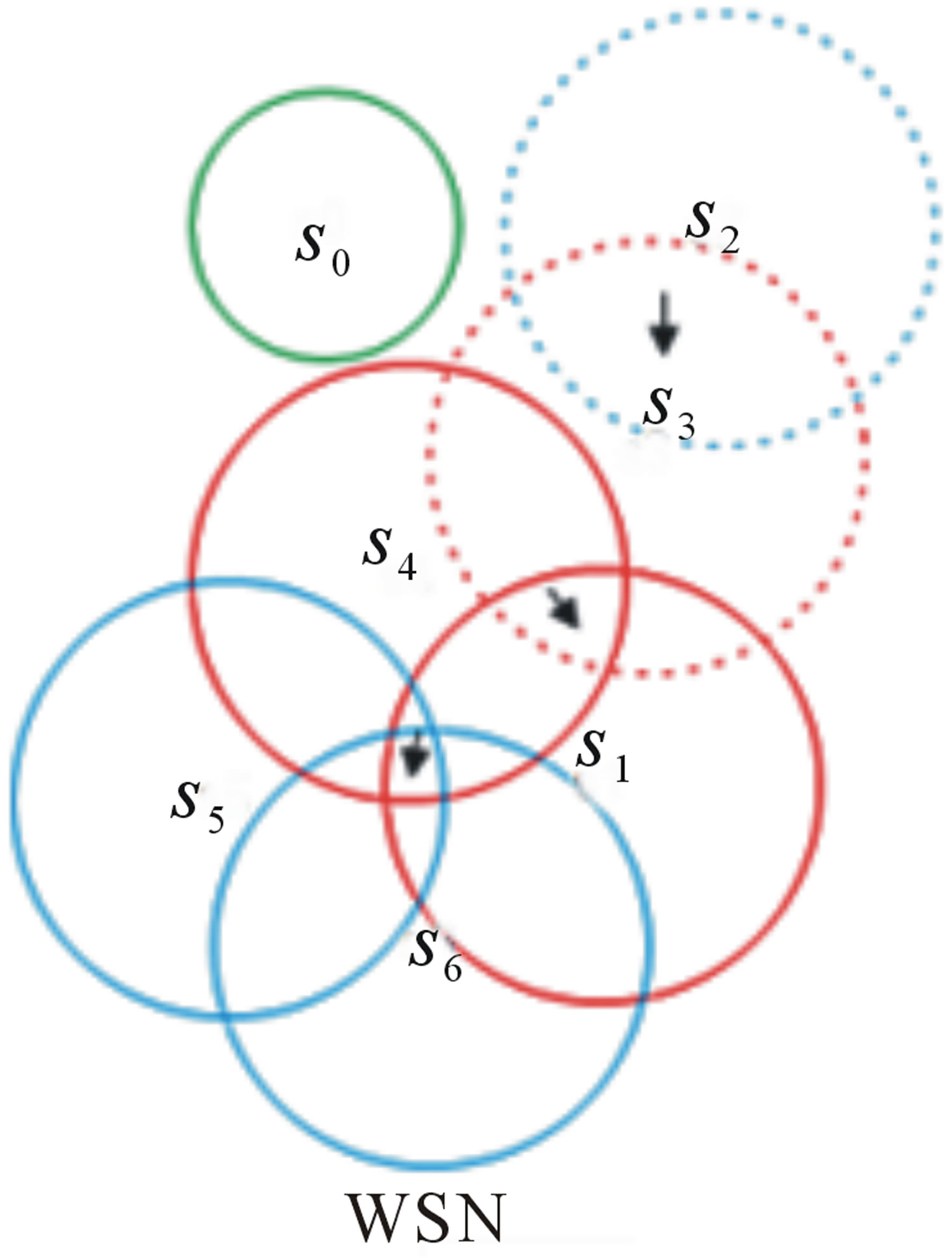
  the coverage degree. Figure 1 shows four groups
 , and
, and . The maximum degree of sensor
  and senor
  is
is  that occurs in the area of intersection, which means that there is one and only one area covered by two sensors and that is the maximal overlapping that could be produced, so sensor
  and
and  create a group of two sensors denoted by
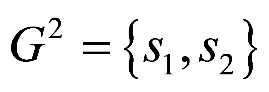 . Sake of convenience, we denote to the group of sensors that build up the WSN by
 which we call it the mother network group or simply the mother group.
2.1. Counting the Sub-Areas of Sensors Group
Here we start by asking, how many sub-areas are generated if  unit disk sensors are partially overlapped? Assuming there is no fully overlapping between sensors, and all sensors are homogenous (sensors have the same sensing range). Say
  is the function to count the number of sub-areas, definitely
 .
. ,
,  ,
,  ,
,  (see Figure 2). What is
 ?
? .
.
Theorem 1: the sub-areas number of a sensors group
 (a)
(a) (b)
(b)
Figure 1. Partitioning the WSN into group.
 is
is
 (1)
(1)
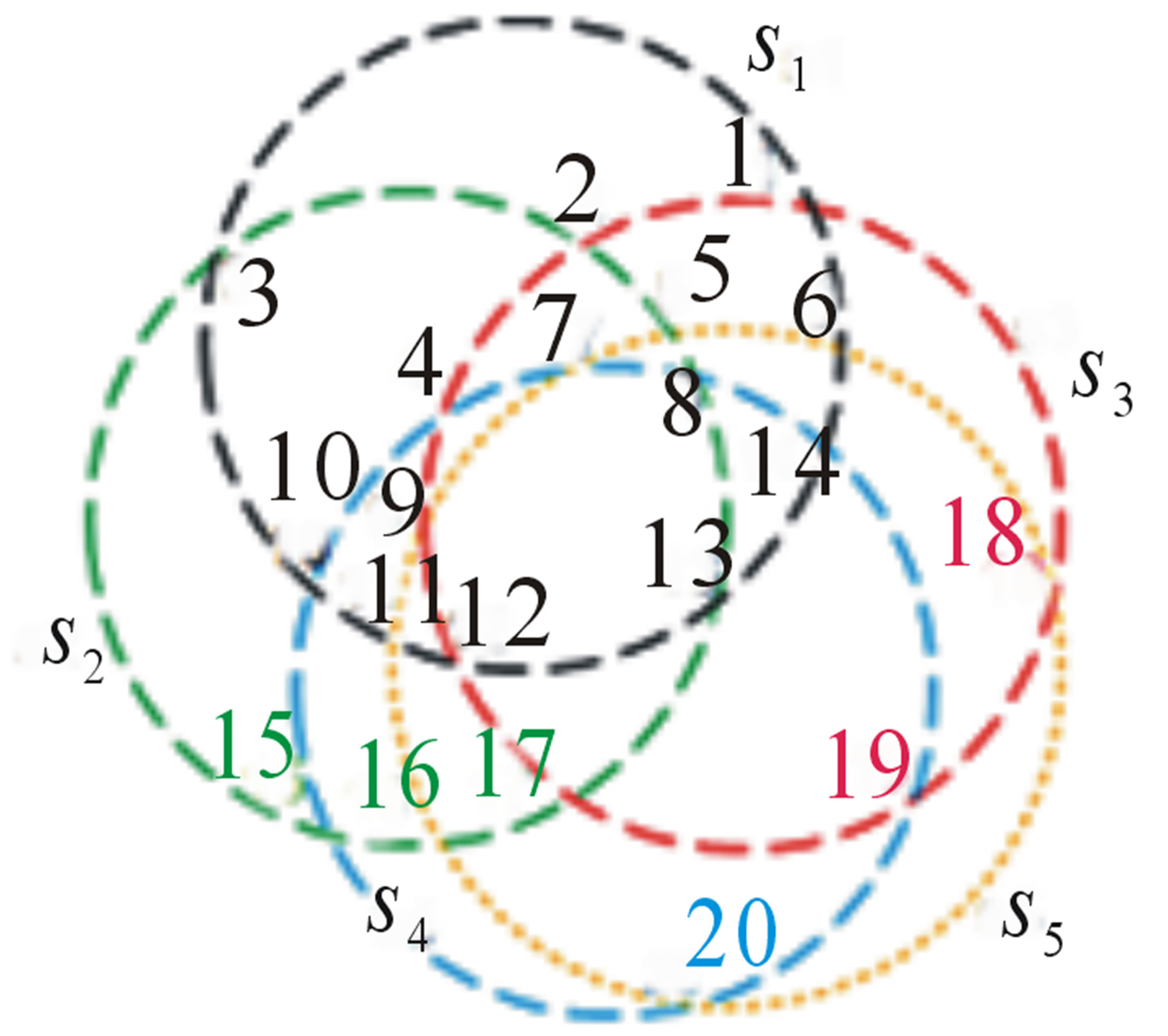
Proof: suppose we have a group of sensors  as shown in Figure 3, we can see that the number of areas inside each sensor’s range is seven. Using Top-down approach from
  to
to , the number of areas for the top sensor
  is seven (red areas namely 1, 2, 3, 4, 5, 6, 7). The number of areas inside the sensor’s range
  are seven, namely (4, 5, 6, 7, 8, 9 10), but the red colored areas, 2, 3, 4, 5, already counted in
 , so there are only 3 blue colored areas inside sensor’s range
 , namely 8, 9, 10. For the sensor
 , it has seven areas inside its sensing range, the 3, 5, 6, 7 are red areas already counted in sensor’s range
 , the area 10 is blue area already counted in sensor’s range
 , thus still two black areas in sensor’s range
 , namely 11, 12. For sensing range of
 , there are seven areas inside it, three are red areas (4, 5, 6), two are blue areas (9, 10), and one area is black (11), so there is still one area only in
  (13). Therefore, the number of areas from top to down is 7 + 3 + 2 + 1 = 13. Generally, counting the sub-areas from top to down, the top sensor contains
 areas, the second sensor inside the group
Figure 2. (a) the number of sub-areas of  (b) the number of sub-areas of
  (c) the number of sub-areas of
  (d) the number of sub-areas of
 .
.
Figure 3. The 13 areas of group .
.
contains  areas, the third sensor contains
  areas… the last sensor contains one area
 . Totally, there are
 of areas. Generally, there count of areas is

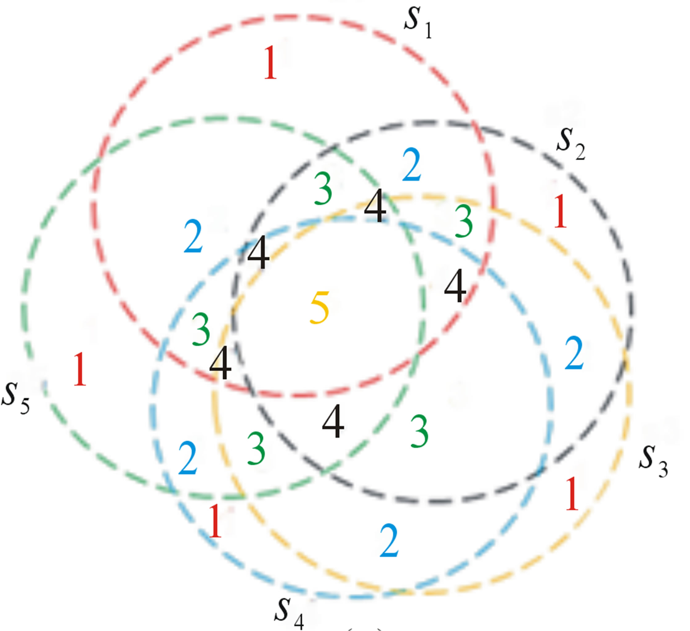
In addition, we can proof theorem 1 by counting the areas of a group basing on the degree of coverage, if an area covered by k sensors then it called k-covered area. For a group  there is only one area is k-covered (the maximum degree of coverage), in the remainder areas, there are k areas are1-covered, k areas are 2-coverd, k areas are 3-coverd… k areas are k-1 covered. Let
  be the number of areas that j-covered inside a group of sensors
 . For example,
  means, there are five areas 1-coverd in
 . In Figure 4" target="_self"> Figure 4(a), the group of sensors
 , the number of 1-coverd areas is five. We can count the sum of areas of sensors group
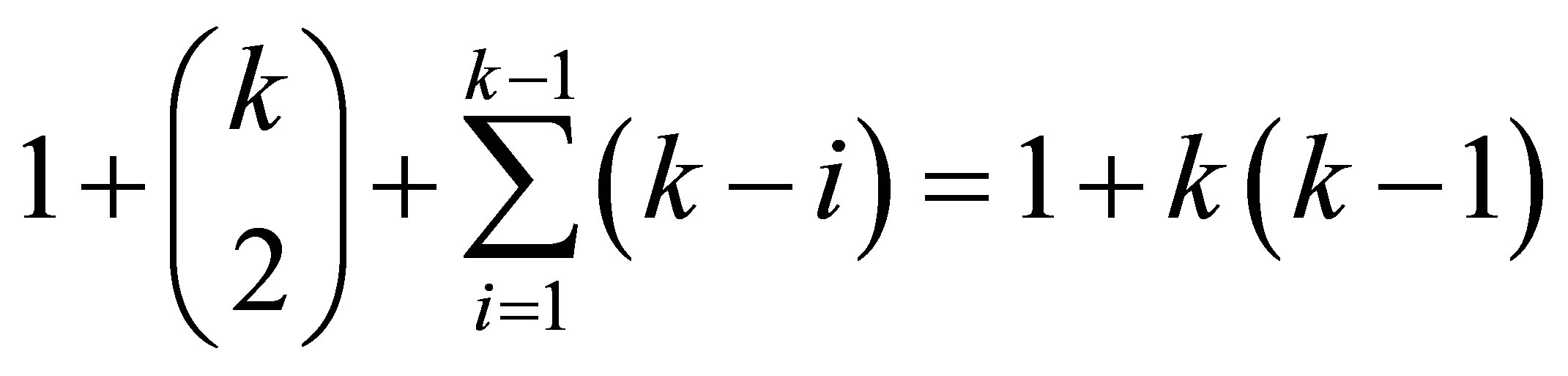
  as below:

Lemma 1: for sensor range belongs to a group , there are only one area k-covered, k area 1-coverd, k areas are 2-coverd, k areas are 3-coverd… and k areas k-1 covered.
Lemma 2: for a group , all sensors have the same characteristics, for example, the number of areas, the degree of coverage for each area, the number of intersection points located on the border of the sensor, and the number of intersection points located inside sensor’s range.
2.2. Counting the Intersection Points of a Sensors Group
Counting the intersection points of k-overlapped sensors is an easy combination problem. Before proving, here we denote to the number of intersection points by , clearly
 ,
,  ,
,  ,
,  ,
,  ,
, … then what is the
 ?
? 
Theorem 2: the number of intersection points of sensors group  is
is
 (2)
(2)
Proof: Assuming that there are k sensors and each sensor has two intersection points with each neighbor sensor, since each sensor has  intersection points with others, applying this method to all sensors, we get the total amount of intersection points as
 . However, while calculating, every single point has been repeatedly counted twice, thus the right answer in regards to the intersection points quantity should be
 .
.
We can use top down approach to calculate the number of intersection points, as shown in the Figure 5(a) .
.  is the top sensor;
  is the bottom sensor of the group. The number of intersection points inside (internal) and on the border of sensing range of the top sensor
  is
is . In the second node
 , there are k-2 of intersection points. In the third node
 , there are k-3 of intersection points. In the fourth node
 , there are k-4 of intersection points, and there is 0 intersection points in the bottom sensor.
Totally the number of intersection points is
Another method to count the intersection points of a group, we can imagine that the number of intersection points as the number of 2-permutation of k sensors, for example, S is a set of overlapped sensors  . The 2-permutation of S is:

 ,
,

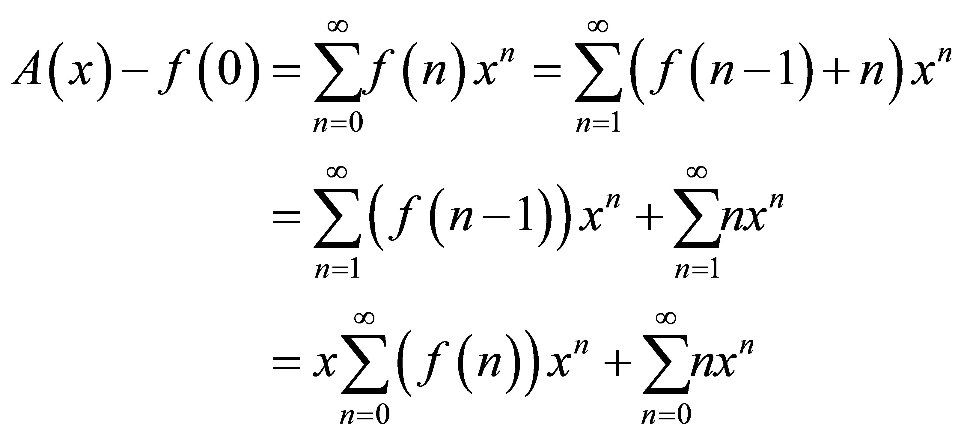
We can use the Recurrence relation to find the number of intersection points of a group of sensors. We can find the recurrence relation of the number of intersection points as below:
 (3)
(3)
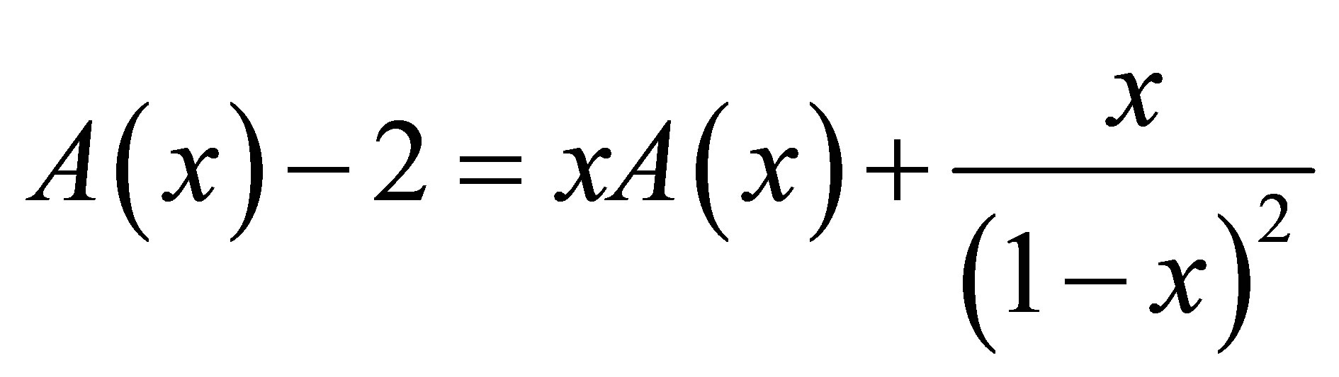
which can be easily solved using generation function [21]. (See the proof of theorem 3), the solution is  , so
, so .
.
2.3. Counting the Number of Intersection Points That Located within the Sensing Rang of a Sensor Associated to a Group (Internal Points and External Points)
In Figure 5(c), we can see that when k = 3 the number of intersection points located in the black sensor are 5, in Figure 5(b) k = 4, the number of intersection points located in the red sensor are 9, when k = 5 the number of intersection points are 14.
Theorem 3: for a group of sensors , the number of intersection points within the sensing range of sensor is
Proof: it is easy to realize that the number of intersection points (internal and external) of the sensor is satisfying the recursive relation:
 (4)
(4)
 (a)
(a) (b)
(b)
Figure 4. (a)  group of sensors, (b)
  group of sensors.
 (a)
(a)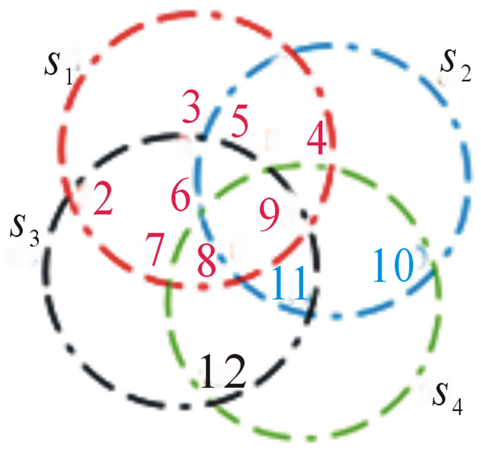 (b)
(b)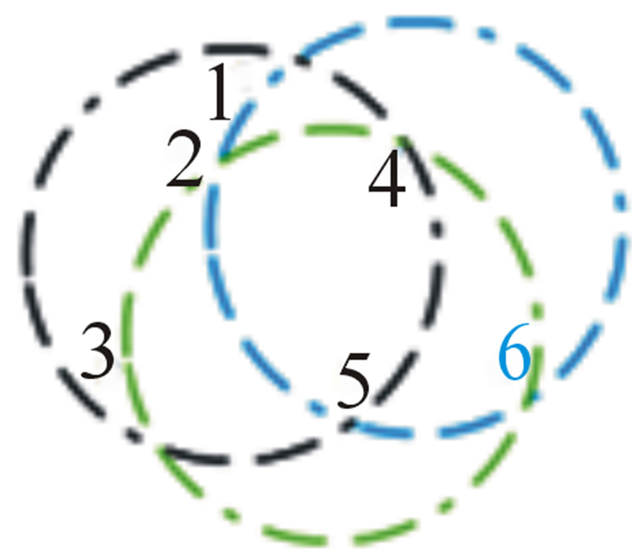 (c)
(c)
Figure 5. (a) Intersection points of group , (b) intersection points of group
 , (c) intersection points of group
 .
.
So finding the solution to this recursive relation is the proof of the theorem.
Suppose the generation function is

In addition, suppose that 
Then

The external intersection points of sensors are the points located on the border of a sensor. However, the internal points are those points located inside the sensors but not on the border.
Lemma 3 (the number of external points): the number of intersection points located on the border of a sensor, which belongs to a group of sensors  is
is  .
.
Proof: from Figure 5, it is easy to realize that the number of intersection points (external) of the sensor is satisfying the recursive relation:

We can solve this relation using generation function as in the proof of theorem 3. Therefore, the solution to this recursive relation is the proof of this theorem
 .
.
Lemma 4 (the number of internal points): the number of intersection points located inside a sensor (not including the points located on the border) is

Proof: from Figure 5, it is easy to realize that the number of intersection points (internal) of the sensor is satisfying the recursive relation:
 (5)
(5)
We can solve this relation using generation function as in the proof of theorem 3. Therefore, the solution to this recursive relation is the proof of this theorem.

From lemma 3, and lemma 4, we get the number of intersection points of a sensor that belongs to a group of sensors  by counting the intersection points located on the border of the sensor (external points) and the intersection points located inside the sensor (internal points).
 (6)
(6)
2.4. Counting the Number of Areas within the Sensing Range of a Sensor That Belongs to a Group 
Theorem 4: The number of areas inside the sensor  that belongs to a group of sensors
  is
is
Proof: it is easy to realize that the number of areas inside the sensor is satisfying the recursive relation:
 (7)
(7)
We can solve this relation using generation function as in the proof of theorem 3. Therefore, the solution to this recursive relation is the proof of this theorem
2.5. Counting the Number of Areas Located within the Sensing Range of a Sensor That Belongs to Multiple Groups
In Figure 1, the network sensors group is:
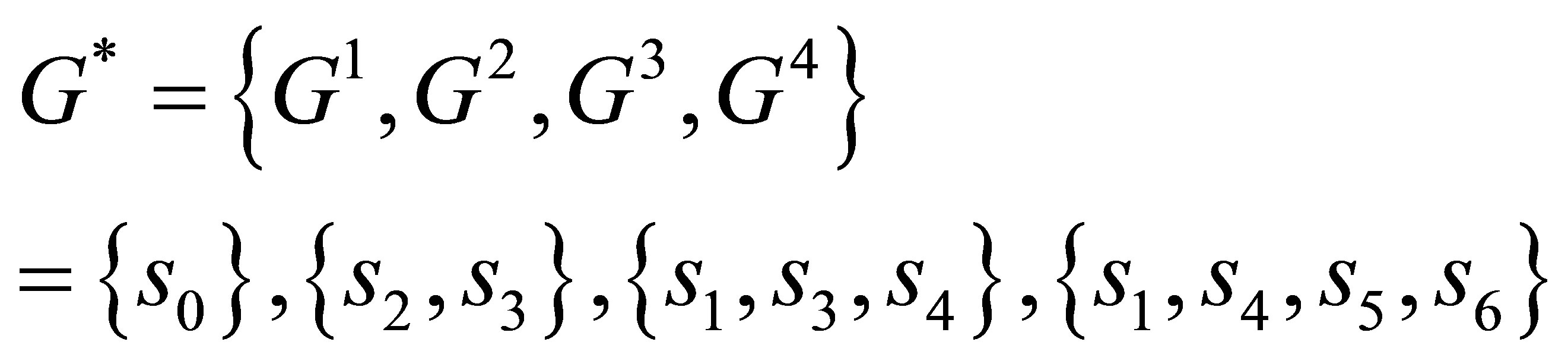
Our goal is to count the number of areas inside the sensor  that associated to multiple groups. The groups to which
  belongs can be defined as following:
Say that  then we can define the mother group of
  as:
as:
 .
.  , where a, b, c are the positive integers numbers that represent the degree of coverage.
As shown in Figure 1 we can define the mother group of sensors ,
,  ,
,  ,
,  ,
,  ,
,  and
and  as below:
Since  only, then the mother group of sensor
  is
is 
Since , then the mother group of sensor
  is
is 
Since , then the mother group of sensor
  is
is 
Since , then the mother group of sensor
  is
is 
Since , then the mother group of sensor
  is
is 
Since , then the mother group of sensor
  is
is 
Since , then the mother group of sensor
  is
is 
It is clearly that the mother group of sensors of the whole network is equal to the union of mother groups of all sensors as shown below:

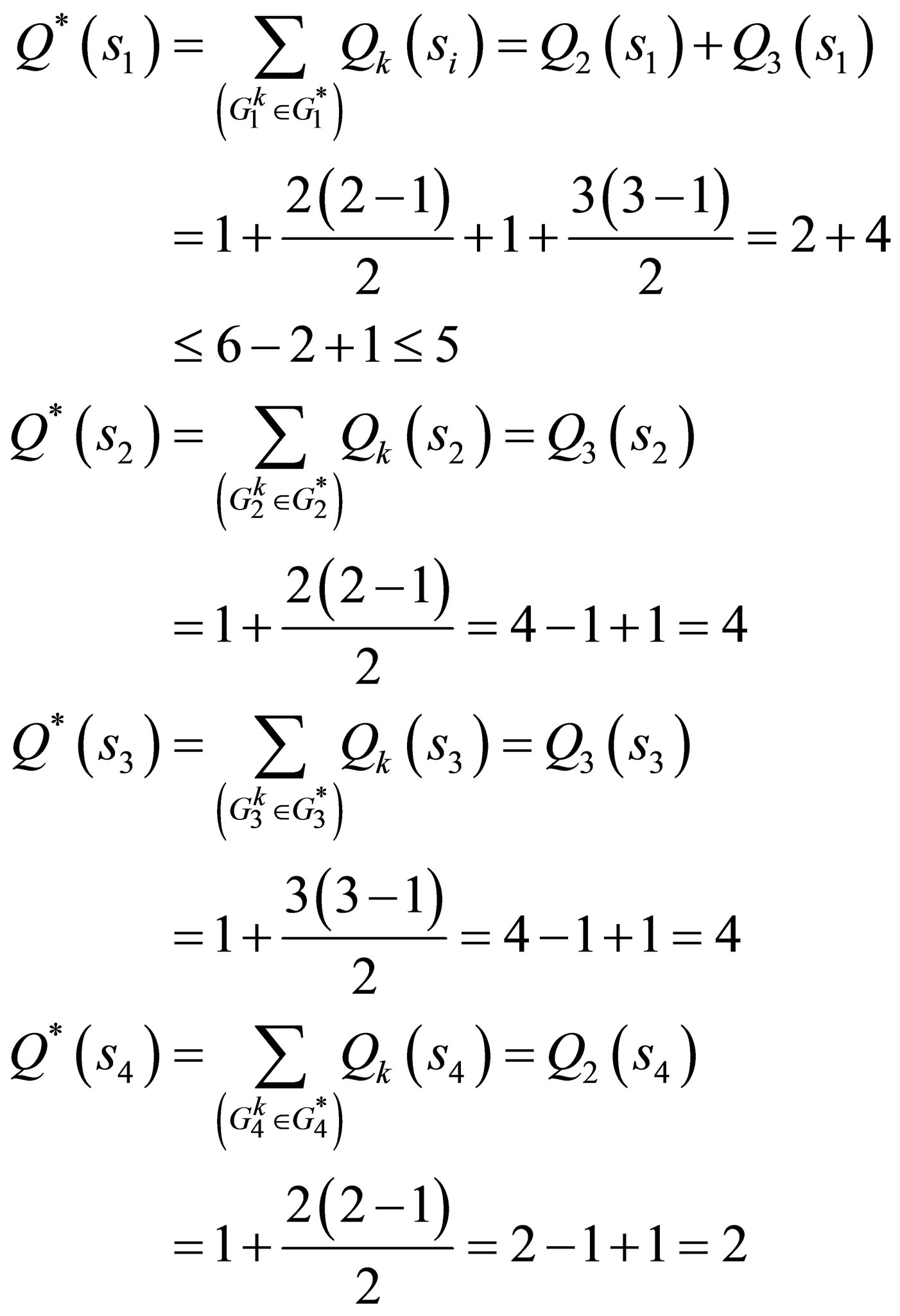
Let us now count the number of areas inside a sensor; these areas are generated by intersection of multiple groups of sensors. For facilitate, let us define  as the number of areas inside a sensor
 , which are generated by overlapping of a group of sensors
 . As explained above, the mother group of
  is
is  , according to theorem the number of areas which created inside
 is
is  (indicated in Figure 6 by numbers 1, 2, 3, 4. The number of areas which are created inside,
  , is
, is .
.
The total number of areas inside a sensor , which, associated to multiple groups is denoted by
 . these areas are created by intersection of sensors belong the mother groups
 .form the first glance, the
  seems like

However, this form is not correct, because  is an element belongs to every sup-group of
  this means that there is one area will be counted
  times. Let us denote the length of mother group by
  which indicates the number of sub-groups inside the mother group of the sensor. So the corrected count of areas inside
 , which belongs to
 , is:
, is:
 (9)
(9)
Below we can count the number of areas of sensors of Figure 7
2.6. Number of Distributed Messages
One of our aims is to find the number of distributed messages that will be generated during communications of sensor  associated to mother group
 . Let us define the number of messages by
 .For ease, let
  be the order of
 .
. Indicates the number of sensors that belong to every sub-group inside the mother group
 , but not including
 , with no repetition, (some sensors might belong to more than one sub-group). For example Figure 1, the order of
  is
is ; the order of
 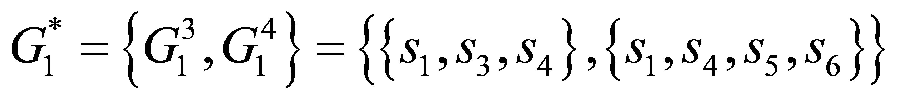 is
is
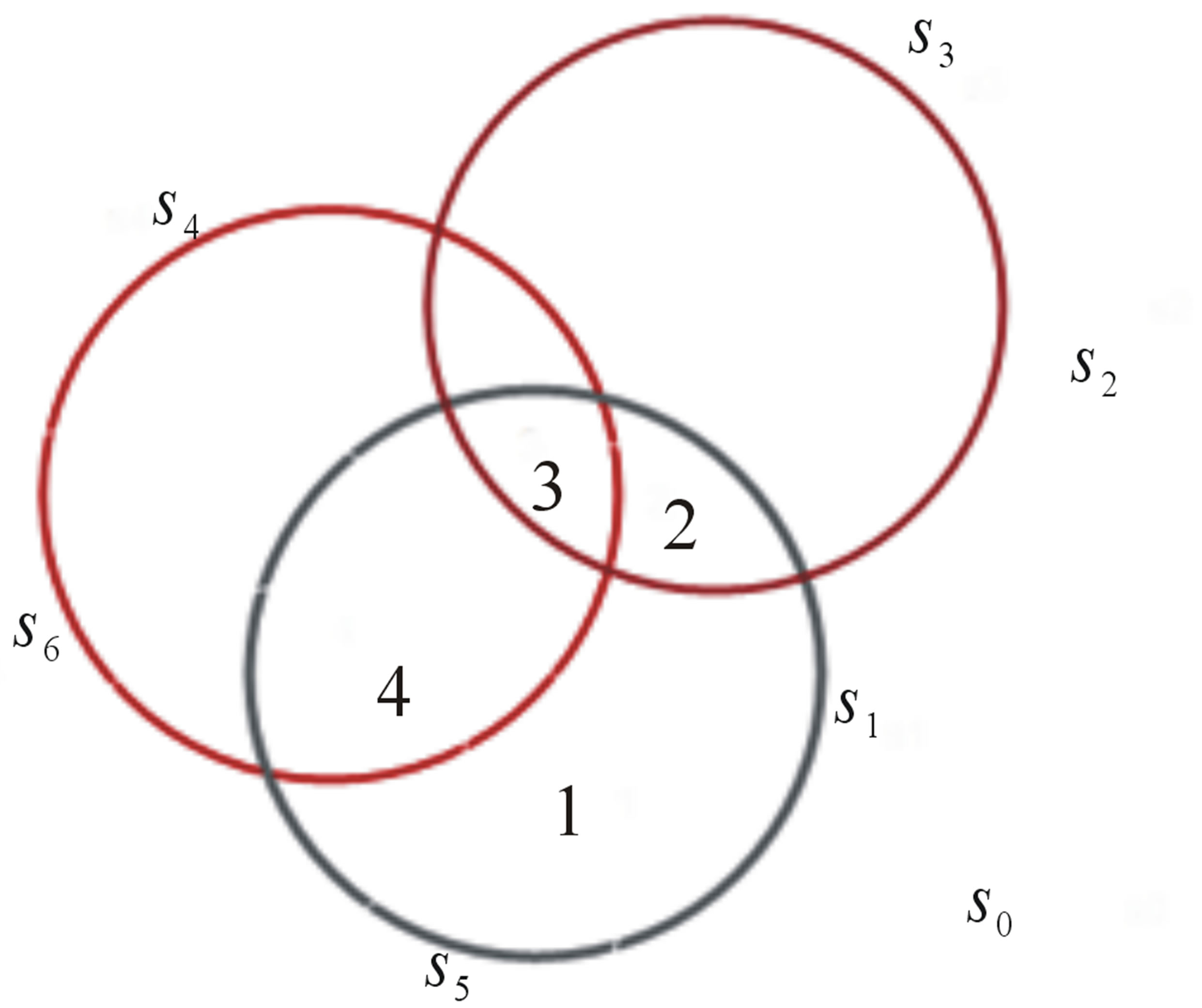
Figure 6. The number of areas inside sensor  by group of sensors
 .
.

Figure 7. Example of groups of sensors.
To generalize this idea, we can write the equation further. We have  associated to the mother group
  , the order of mother group of
  is as the equation below
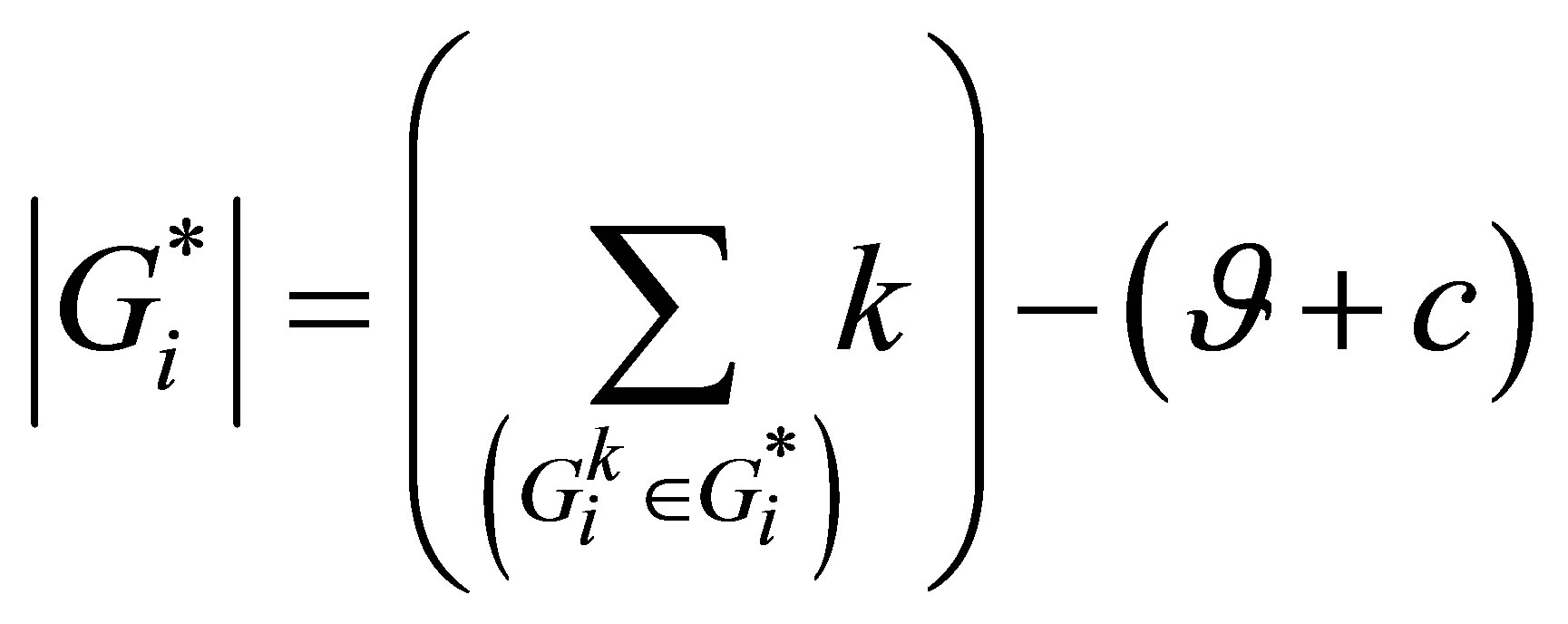
Here the integer number  is the count of subgroups of
 . In addition, c is the repetition.
It is clear that  since the degree of sub-group
  is one and the there is only one sub-group. Applying this calculation to mother group of sensor
 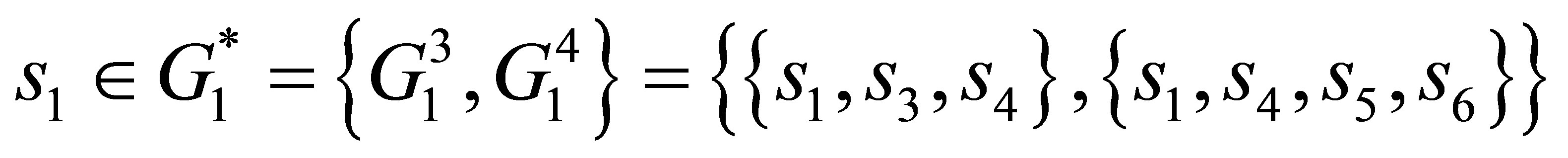 , the order
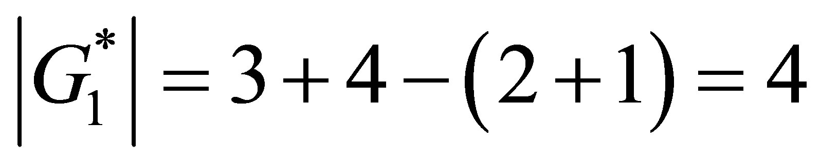 .
.
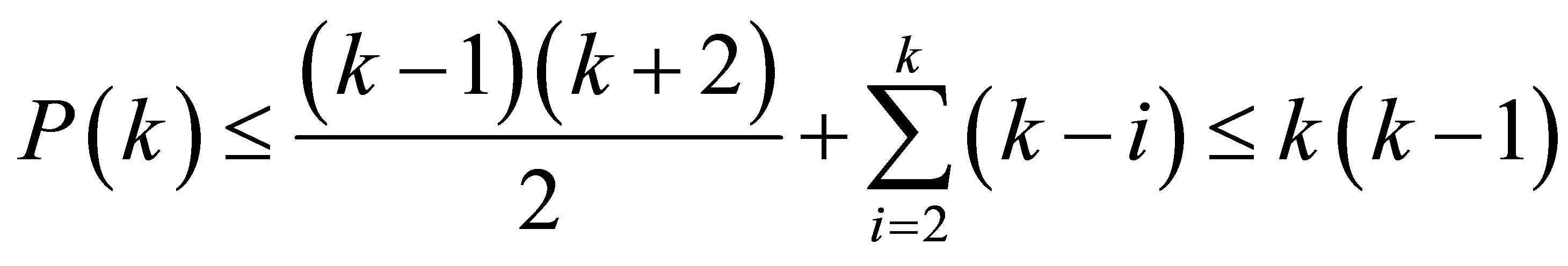
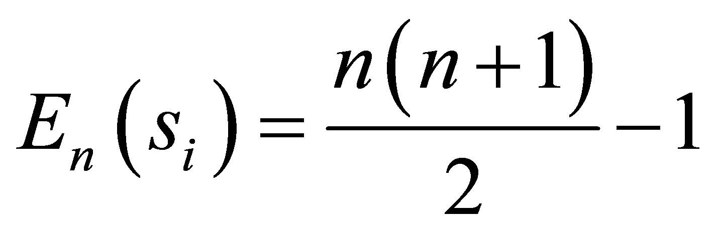
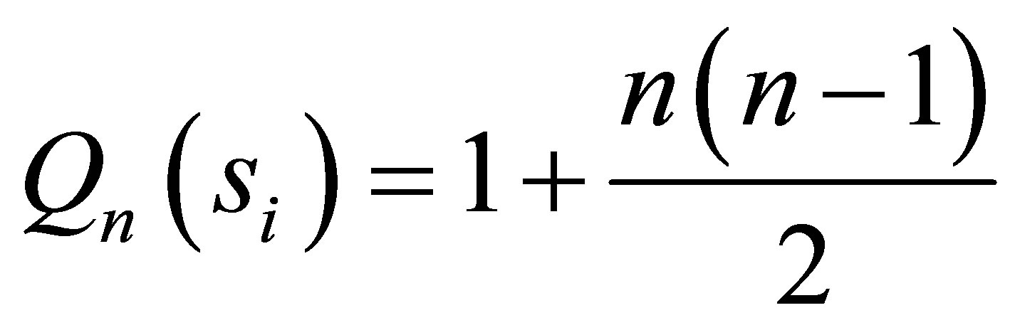
Theorem 4: The number of distributed messages sent form , associated to a mother group
 , is
, is 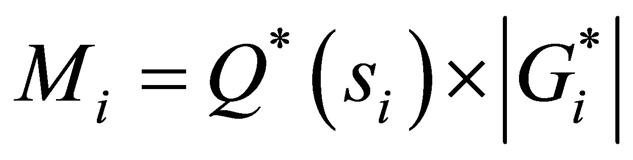
Proof: The number of messages depends on the degree of overlapped sensors. The more the degrees of coverage are, the more the areas will be generated. Therefore, the more messages will be generated. When a target moves within the range of a sensor , it will send notification messages to all neighbors but certainly not to itself. Since the sensor contains a certain number of intersection areas and a certain number of sensors cover these areas, the sensor will send a notification message to all the sensors that cover the same area.
  is the number of areas inside
  which belongs to
 , and
, and  is the order of
 , then
 .
.
The number of messages of the network in Figure 1

3. Conclusion
We had introduced a new method of organizing the sensors of WSN into groups, which would be easy to manage and communicate. This new idea could be applied in coverage algorithms in order to control one node and one target at any given moment, and it could be used to speed up the routing algorithms as well.
4. Acknowledgements
The authors would like to acknowledge The National Natural Science Foundation of China, the National Science Technology Major Project and the China Scholarship Councilfor their supports.
REFERENCES
- http://en.wikipedia.org/wiki/Wireless_sensor_network
- C.-Y. Chong and S. P. Kumar, “Sensor Networks: Evolution, Opportunities, and Challenges,” Proceedings of the IEEE, Vol. 91, No. 8, 2003, pp. 1247-1256. http://dx.doi.org/10.1109/JPROC.2003.814918
- E. Zanaj, M. Baldi and F. Chiaraluce, “Efficiency of the Gossip Algorithm for Wireless Sensor Networks,” Proceedings of the 15th International Conference on Software, Telecommunications and Computer Networks (SoftCOM), Split-Dubrovnik, Croatia, September 2007.
- “Mems and Nanotechnology.” http://www.memsnet.org/
- I. F. Akyildiz, W. Su, Y. Sankarasubramaniam and E. Cayirci, “Wireless Sensor Networks: A Survey,” Computer Networks, Vol. 38, No. 4, 2002, pp. 393-422. http://dx.doi.org/10.1016/S1389-1286(01)00302-4
- D. Estrin, R. Govindan, J. S. Heidemann and S. Kumar, “Next Century Challenges: Scalable Coordination in Sensor Networks,” Proceedings of ACM MobiCom’99, Washington, August 1999.
- J. M. Kahn, R. H. Katz and K. S. J. Pister, “Next Century Challenges: Mobile Networking for “Smart Dust,” Proceedings of ACM MobiCom’99, August 1999.
- A. Mainwaring, J. Polastre, R. Szewczyk and D. Culler, “Wireless Sensor Networks for Habitat Monitoring,” First ACM International Workshop on Wireless Workshop in Wireless Sensor Networks and Applications (WSNA 2002), August 2002. http://dx.doi.org/10.1145/570738.570751
- S. C.-H. Huang, S. Y. Chang, H.-C. Wu and P.-J. Wan, “Analysis and Design of Novel Randomized Broadcast Algorithm for Scalable Wireless Networks in the Interference Channels,” IEEE Transactions on Wireless Communications, Vol. 9, No. 7, 2010, pp. 2206-2215. http://dx.doi.org/10.1109/TWC.2010.07.081579
- H. H. Zhang and J. C. Hou, “Maximising α-Lifetime for Wireless Sensor Networks,” 2007.
- M. Cardei and D. Z. Du, “Improving Wireless Sensor Network Lifetime through Power Aware Organization,” Wireless Networks, Vol. 11, No. 3, 2005, pp. 333-340. http://dx.doi.org/10.1007/s11276-005-6615-6
- S. Poduri and G. Sukhatme, “Constrained Coverage for Mobile Sensor Networks,” IEEE International Conference on Robotics and Automation, New Orleans, 26 April- 1 May 2004, pp. 165-172.
- A. Chen, S. Kumar and T.-H. Lai, “Designing Localized Algorithms for BarrierCoverage,” MOBICOM. ACM, September 2007.
- X. Bai, Z. Yun, D. Xuan, T. Lai and W. Jia, “Optimal Patterns for Four-Connectivity and Full Coverage in Wireless Sensor Networks,” IEEE Transactions on Mobile Computing, 2008.
- J. Wu and S. Yang, “Coverage and Connectivity in Sensor Networks with Adjustable Ranges,” International Workshop on Mobile and Wireless Networking (MWN), August 2004.
- M. Cardei, J. Wu, N. Lu and M. O. Pervaiz, “Maximum Network Lifetime with Adjustable Range,” IEEE International Conference on Wireless and Mobile Computing, Networking and Communications (WiMob’05), August 2005.
- M. Cardei, M. T. Thai, Y. Li and W. Wu, “Energy-Efficient Target Coverage in Wireless Sensor Networks,” Proceedings of IEEE Infocom, 2005.
- M. Cardei and D.-Z. Du, “Improving Wireless Sensor Network Lifetime through Power Aware Organization,” Vol. 11, No. 3, 2005, pp. 333-340.
- J. K. Hart and K. Martinez, “Environmental Sensor Networks: A Revolution in the Earth System Science?” EarthScience Reviews, Vol. 78, 2006, pp. 177-191. http://dx.doi.org/10.1016/j.earscirev.2006.05.001
- Y. Ma, M. Richards, M. Ghanem, Y. Guo and J. Hassard, “Air Pollution Monitoring and Mining Based on Sensor Grid in London,” Sensors, Vol. 8, No. 6, 2008, p. 3601. http://dx.doi.org/10.3390/s8063601
- E. Kreyszig, “Advanced Engineering Mathematics,” John Wiley & Sons, INC, 1999.
Distributed messages of network shown in Figure 1.

NOTES
*This paper is supported by The National Natural Science Foundation of China (NO.61272472, 61232018, 61202404) and the National Science Technology Major Project (NO. 2012ZX10004301-609).