Journal of Sensor Technology
Vol.2 No.1(2012), Article ID:17934,15 pages DOI:10.4236/jst.2012.21005
Multidimensional Median Filters for Finding Bumps in Chemical Sensor Datasets
1Department of Biostatistics, Roswell Park Cancer Institute, SUNY University at Buffalo, Buffalo, USA
2Department of Mathematics and Statistics, Georgetown University, Washington DC, USA
3Department of Statistics, Carnegie Mellon University, Pittsburgh, USA
Email: jcm38@buffalo.edu
Received October 14, 2011; revised November 14, 2011; accepted December 6, 2011
Keywords: Bump Hunting; Image Analysis; Spatial Smoothing; Feature Detection; Mathematical Morphology
ABSTRACT
Feature detection in chemical sensors images falls under the general topic of mathematical morphology, where the goal is to detect “image objects” e.g. peaks or spots in an image. Here, we propose a novel method for object detection that can be generalized for a k-dimensional object obtained from an analogous higher-dimensional technology source. Our method is based on the smoothing decomposition, Data = Smooth + Rough, where the “rough” (i.e. residual) object from a k-dimensional cross-shaped smoother provides information for object detection. We demonstrate properties of this procedure with chemical sensor applications from various biological fields, including genetic and proteomic data analysis.
1. Introduction
Numerous chemical sensor platforms and technologies require image analysis techniques to isolate the signal from the associated noise in the sensor. In a one-dimensional chemical sensor setting, for example, several technologies produce spectra where scientists can gain information from associated peaks, or grayscale images where the features appear as streaks or lines. Meanwhile, in a two-dimensional setting, associated technologies produce images whose features are spots. Such image analyses usually involve methods where the goal is to identify and quantify the size of an image feature or object, i.e. feature detection and quantification.
Feature detection in multi-dimensional images is an area of great interest in a variety of applications, ranging from astronomy to proteomics [1-7]. Proposed methods employ image segmentation techniques such as watershed methods, thresholding operators, and wavelet reconstruction methods to locate the features contained in a one-dimensional or two-dimensional image. Further, feature detection has a growing body of research in larger high-dimensional datasets, as well; see, for example, [8, 9]. The algorithms and methods proposed, however, usually apply solely to the application and technology of interest and may not be applicable to images of other forms or varying dimensionality.
Determining the locations and boundaries associated with various chemical sensor features has been a problem considered by computer scientists and engineers (under the guise of image analysis), as well as mathematicians and statisticians (via mathematical morphology). Mathematical morphology (MM) is the science of analyzing and processing geometric structures (e.g. local maxima) in digital images via various processing techniques (e.g. local maxima) in digital images via various processing techniques [10-15]. Examples of common MM functions include opening, closing, thinning, binning, thresholding, and watershed methods, and have been employed in numerous applications including pedestrian detection [16], tumor mass detection [17], and facial feature detection [18,19]. A key component in MM lies in the choice of structuring element, i.e. the shape used to interrogate the image; its two main descriptive characteristics are its shape and size. In digital images, the structuring element scans the image and alters the pixels in its window content using basic operators similar to Minkowski addition. Since the goal is commonly to smooth images by removing the statistical noise, the usual practice is to choose a window which is (hyper-) cubical or (hyper-) spherical. Since our goal is feature detection rather than data smoothing, we instead propose a MM technique with a “cross” shaped structuring element in conjunction with residual analysis to aid in bump finding in chemical sensoring images. We have found that, by choosing the window to be (hyper-) crossical (i.e. shaped like a multi-dimensional cross), the resulting residual image also contains crosses whose centers identify the locations of local maxima.
This paper combines aspects of feature detection, data smoothing, and residual analysis to develop a new bump detection method for not only oneor two-dimensional images, but k-dimensional images for any . Thus, not only is this method straightforward, but it can also be applied universally to higher-dimensional images, providing researchers with a detection and quantification method for any chemical sensor technology whose features of interest are bumps.
2. Theoretical Model
In our method, a specialized median (referred to hereafter as an s-median) smoother is developed, where the s-median determines the median associated with the intensity values that lie spatially in the cross-shaped structuring element. Consider a k-dimensional (kD) image represented by , where x is a point location in the Cartesian coordinate system. We let
  denote the kD smoothed image obtained by using an s-median operator with “arms” of length
  on
on ; window size examples are provided in Figure 1.
 , for example, refers to the smoothed image that results from applying the the 5- pixel cross (see Figure 1(a)) s-median structuring element across
 . In this case, the center pixel within any
  window in
  is replaced with the associated median value from the 5-pixel cross. Similarly, applying a 9-pixel cross s-median (as shown in Figure 1(b)) across
  produces
 .
.
After applying this s-median throughout the raw image, we examine the associated residual image,  , to obtain information regarding bump detection and quantification. The
  image contains k-dimensional cross features, where associated image local maxima identify the associated bump center, and local minima outline the shape of the bump. We can use this information, for example, to identify peaks and their associated area in one-dimensional applications involving spectral data, or spot detection and quantification in two-dimensional images. Sections 2.1 and 2.2 introduce the theoretical underpinnings for our method and demonstrate the procedure for continuous and discrete functions, while Section 2.3 extends these ideas to study the behavior of the smedian operator in the presence of noise.
2.1. Computation on Continuous Functions
This section develops the theoretical underpinnings for  and, subsequently,
  in the context of continuous functions. We derive
  for 1D and 2D theoretical models by characterizing the the median operator
 (a) (b)
Figure 1. Examples of window shapes in 2D: Window shape, often called the structuring element in morphology, refers to the pixels used to compute the median for smoothing. The window shapes are shaded in grey. (a) A 3 × 3 s-median cross window consisting of five pixels. This s-median replaces the intensity in pixel location “5” with the median intensity of the grey pixels (i.e. in locations 2, 4, 5, 6, 8); (b) A 5 × 5 s-median cross window consisting of nine pixels. The s-median image in pixel location “13” is obtained by computing the median intensity of the grey pixels (locations 3, 8, 11, 12, 13, 14, 15, 18, 23).
via the function mapping between input and output values.
2.1.1. One-Dimensional Continuous Functions
Let  and
and  denote the cumulative density function (cdf) and probability density function (pdf), respectively, for the a random variable
  evaluated at the point
 ; analogously, we denote the cdf and pdf for a random variable
  at point
 . Let
. Let  be a function that maps from the support set
  (for the random variable
 ) to the support set
  (for the random variable Y). For our applications,
  is obtained from an optical device such as a charge-coupled device camera or laser scanner. Our goal is to obtain an expression for
  [and thus
 ] which then determines the median of
 ,
,  , i.e.
  satisfies
  . Note that, in our notation for one dimension,
  at a given location, x. Thus, for simplicity, we will denote
  as
as  (or
(or ) with the implicit understanding that
  (or
(or ) is also a function of k and c.
2.1.2. Monotone Case
Consider the case where  is strictly monotone on the interval
 . Then, for
  increasing,
while, for  decreasing,

Strict monotonicity in  implies its invertibility for any
 , i.e.
 ; in particular, by definition of
 , we have
 . Hence, in the monotone case,
  , where
  denotes the median associated with the random variable
 , and “
 ” denotes statistical equivalence as defined in [20], p. 36. Thus, the median for
  is equivalent to the function evaluated at the median for
 ; in short,
 .
.
2.1.3. Piecewise Monotone Case
For the piecewise monotone situation, we define
 as an open interval
  with
with
 . Let
. Let 
 , be the smallest collection of disjoint open intervals such that
  is strictly monotone on each
 . By definition,
  is strictly monotonically increasing on
  if, for any two values
  such that
 ,
,  holds. Analogously,
  is strictly monotonically decreasing if
  for
for  such that
 . Note that continuity may not be enough for the
  to be countable, where we define countability as in [21]. Further, we assume strict monotonicity in the function,
 . We define the interval,
where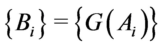 . While the sequence
  partitions
 ,
,  does not necessarily partition
 ; e.g., see Figure 2, where
  and
and .
.
Let , i.e. the
  th decomposition of
 , and
, and  defines the indicator function of
  by
by  (0) if
  is (not) in the interval
 . By definition,
  is strictly monotone. Thus, for
 , we have
 , implying that any function
  can be decomposed into the sum of its strictly monotone components,
 . Accordingly, we see that
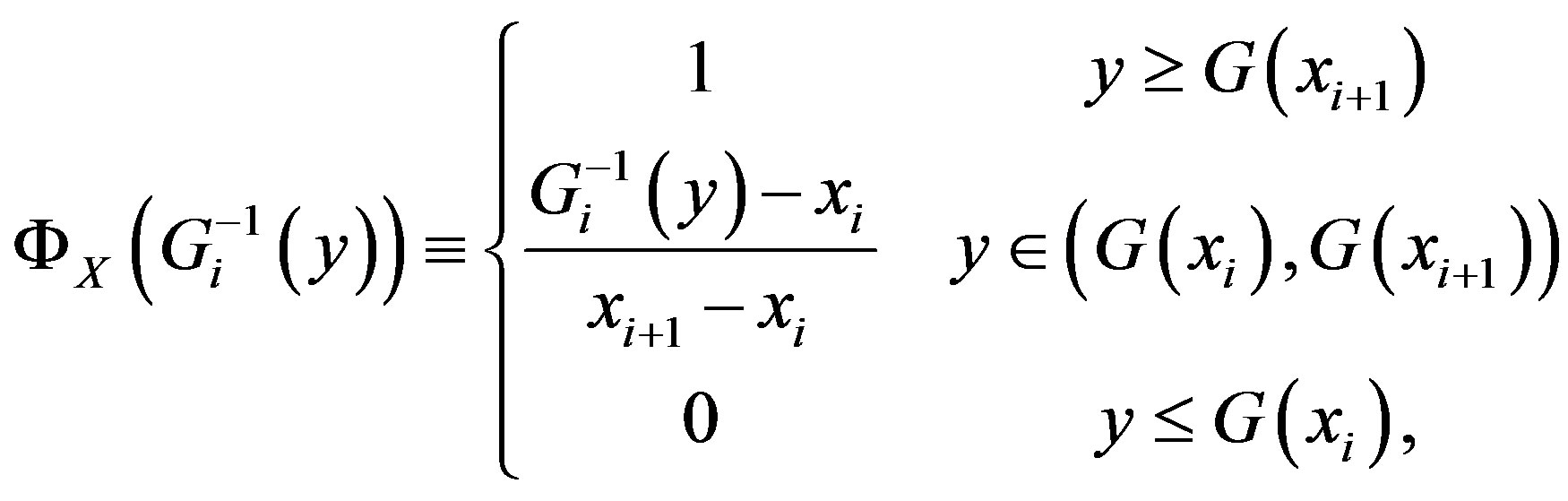
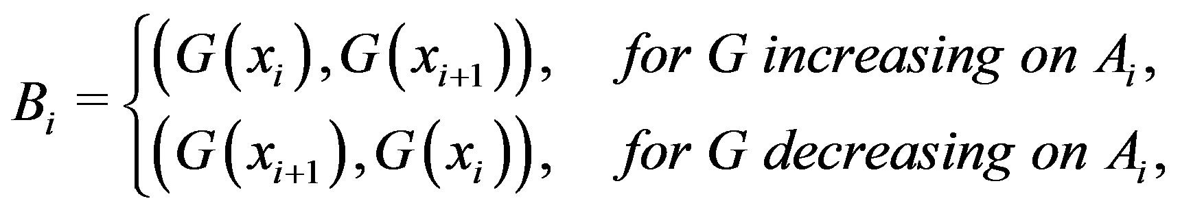
 , where, for
increasing on ,
,
 x
x
Figure 2. Partition: G(x) = x3 – x, where . The dashed horizontal lines denote the {Ai} partition of the x axis, while the dashed vertical lines denote the {Bi} intervals on the y axis.
and, for  decreasing on
 ,
,

For all but the most simple functions, there is no closed form solution by which to define . Nevertheless, the above equations will allow for the calculation of
  and thus
  using computational methods.
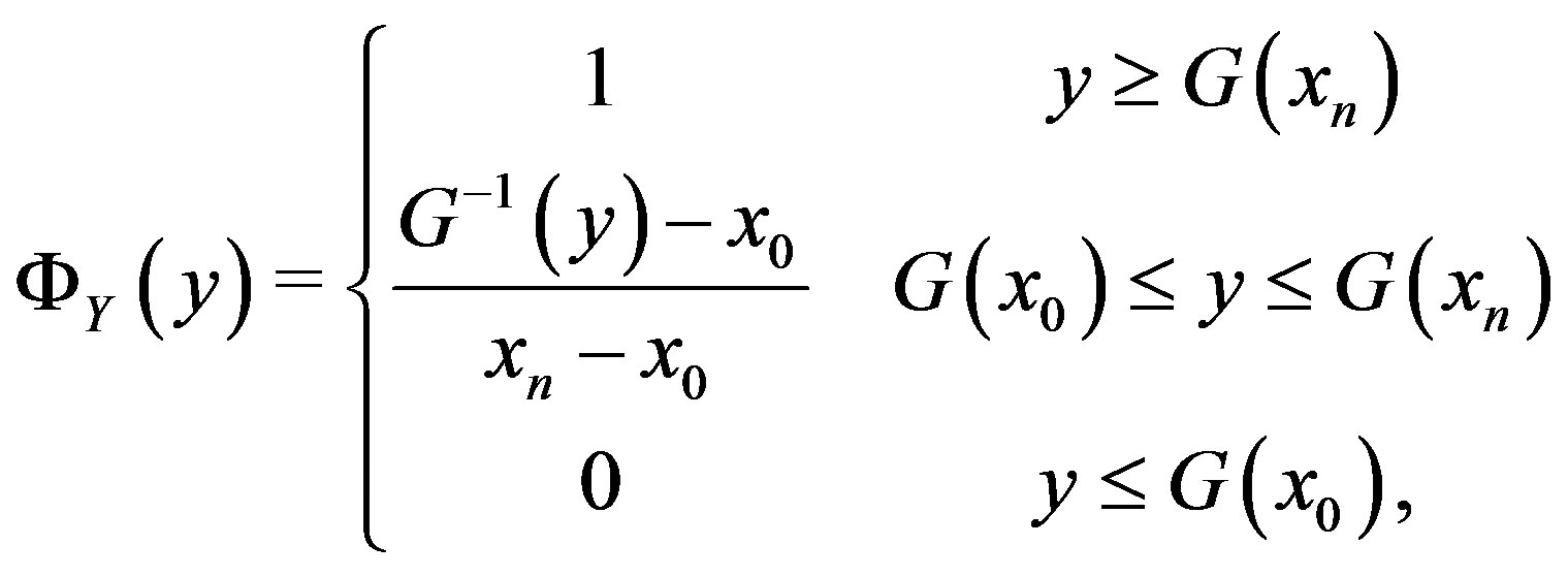
2.1.4. Two-Dimensional Continuous Functions
In the 2D continuous case, we introduce the function  where the goal is to obtain an expression for
 . From standard probability theory such as in
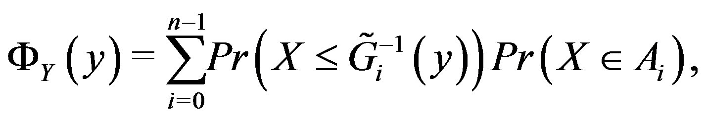
[22], we have , where
 and
and  is the joint pdf for
  and
and . Note that this is the general case for obtaining the cdf of
  in terms of
  and
and . For our specialized median, however, our sample space for
  and
and  must be defined in terms of another parameter, say
 , where
  controls the width of the smoothing window in each dimension. Figure 3 illustrates an example sample space over which to compute
 . Since it is difficult to generalize
 , we cannot generalize this situation to provide an explicit calculation for the median of
 . Nevertheless, computational

Figure 3. 2D continuous sample space: The sample space for the random variables in the 2D continuous setting. This sample space allows us to compute the cdf for Z and thus the specialized median. The sample space is defined in terms of the parameter W.
methods can be used to compute MZ and thus .
.
2.2. Computation on Discrete Functions
Let  denote a “discrete” function, i.e. a function with discrete/countable realizations from the continuous function
 . By definition,
  is a function that maps from the support set
  (of the discrete random variable X) to the support set
  (for the discrete random variable Y). This section considers computational results associated with
  and its impact on the s-median.
2.2.1. One-Dimensional Discrete Functions
Let  and
and  denote the discrete cdf and probability mass function (pmf), respectively, for the arbitrary random variable
  evaluated at the point
 . Let
. Let  be as defined above. The calculation of the s-median proceeds by assuming
  Discrete Uniform(
 ) as defined in [23], and then computing
  based on the function,
 . Thus, the machinery developed in Section 2.1 can be applied to compute
 .
.
We can analogously represent  using discrete random variables
  and
and  as we did for the continuous case, namely
where  indicates probability. If we assume that X~ Discrete Uniform(
 ), then

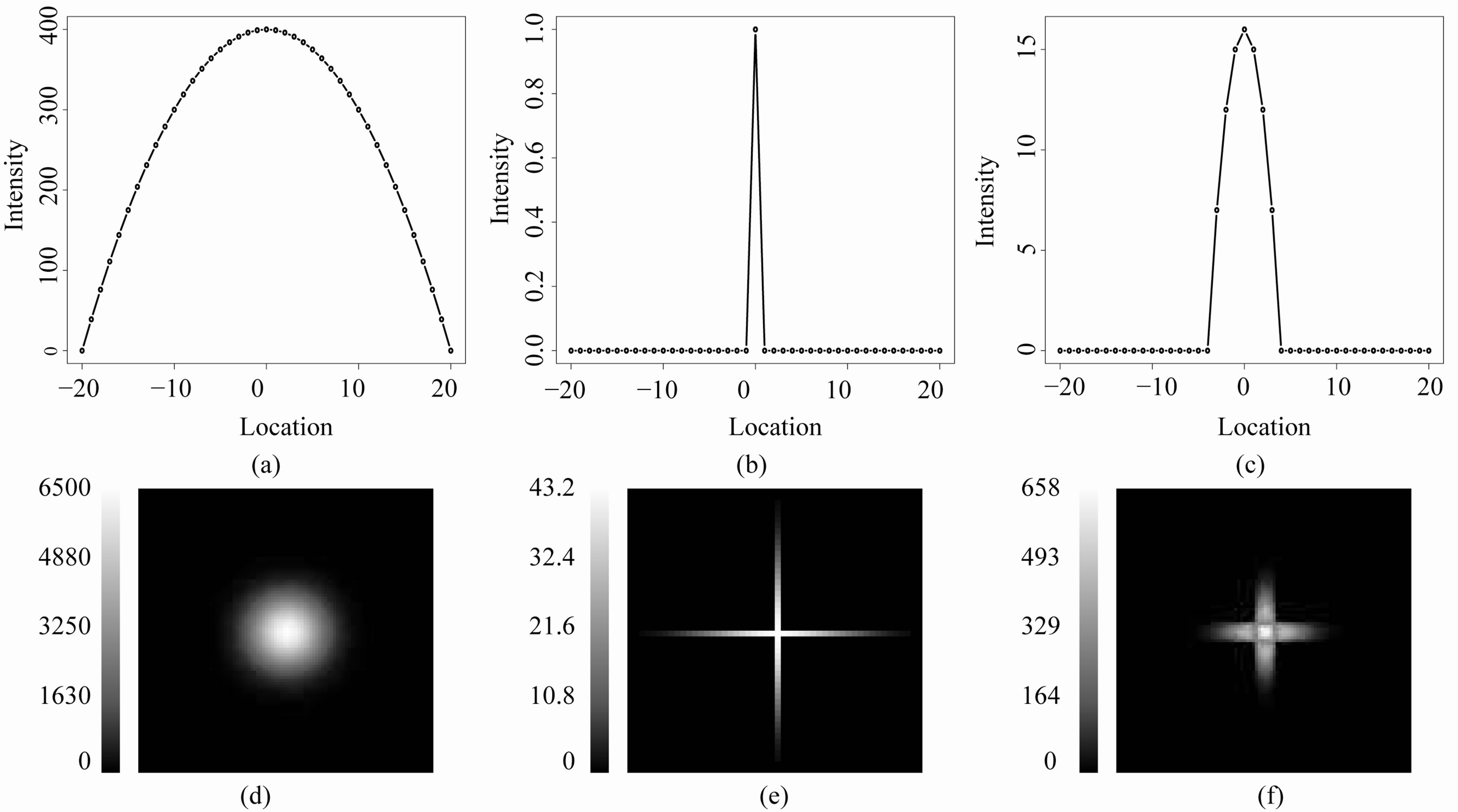
Figure 4. Rk,c for an image I of a single mountain: (a) An image of a 1D mountain generated by I1(x) = –x2 + 400, where x consists of the integers between –20 and 20 (i.e. 41 points); (b) R1,1, i.e. the residual image associated with I1 when applying a smoothing window of three points (c = 1). All of the residuals equal 0 except for the residual intensity at the center of the mountain; (c) R1,7, i.e. the residual image associated with I1 when applying a smoothing window of 15 points (c = 7). The residuals are greater than 0 at the location of the top of the mountain and several adjacent locations; (d) A 100 × 100 pixel image of a two-dimensional mountain generated by ; (e) R2,2, i.e. the residual image associated with I2 using a 5 × 5 s-median where the smoothing window consists of nine pixels (c = 2). The characteristic “cross” is clearly present in this image; (f) R2,7, i.e. the residual image associated with I2 using a 15 × 15 s-median where the smoothing window contains 29 pixels (c = 7). Here, the cross is wider than that appearing in R2;2, but the arms are not as long.
and  with
with  and
and 
denoting the ceiling and floor functions, respectively.
For the special case of a strict monotone discrete function  on the full interval
 ,
,

 does not depend on the direction of monotonicity for
 . Figures 4(a)-(c) show the images from our technique applied to a simple one-dimensional discrete piecewise monotone function.
2.2.2. Two-Dimensional Discrete Functions
For the 2D discrete case, we define the sample space with the following definition.
Definition 2.1 Let  be a discrete uniform on
 ,
,  be a discrete uniform on
 , and (x*, y*) be a fixed point such that x* and y*
 , respectively. Then let
  be of the form,
Figure 5 illustrates the associated sample space. With this definition, the derivation of the s-median for  follows analogously to the 2D continuous case (which is analogous to the 1D case).
Let  define a mapping from the support sets
  and
and , of the random variables X and Y respectively, to the support set
 , for the random variable Z. We define the functions,
  and
and
 , such that
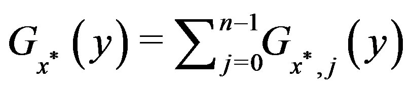 ,
,
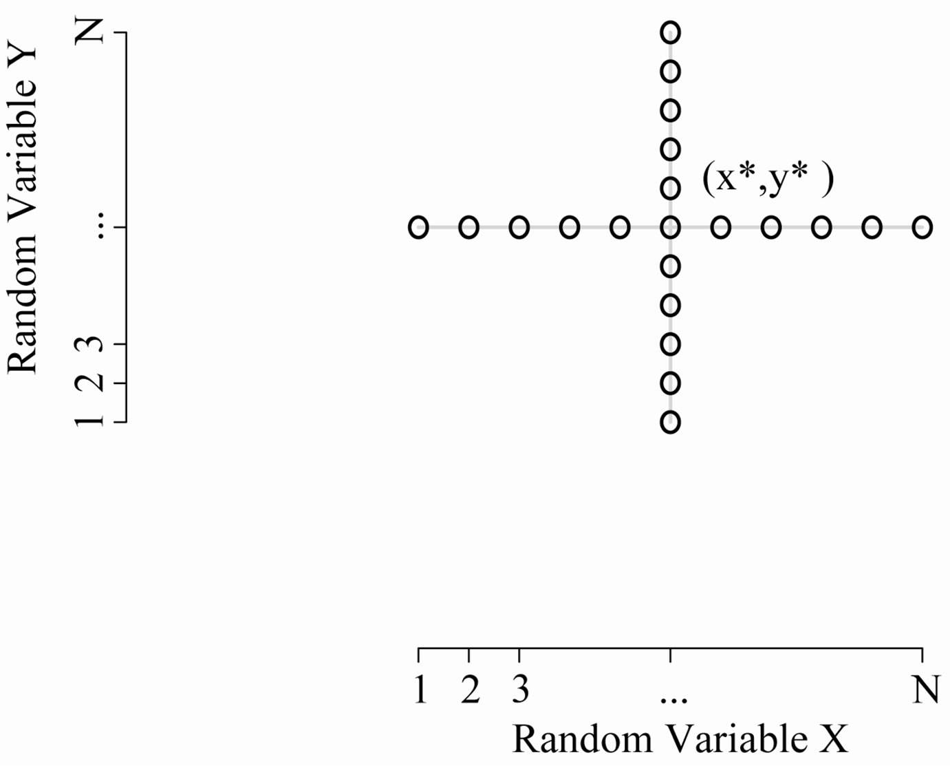
Figure 5. 2D discrete sample space: The discrete uniform random variables in the 2D setting. The center point is at the coordinate, (x*; y*).
and , where
  is the the smallest set of disjoint open intervals such that
  is strictly monotone on each
 ,
, ; and
; and  is the smallest set of disjoint open intervals such that
  is strictly monotone on each
 ,
, . In this setting,
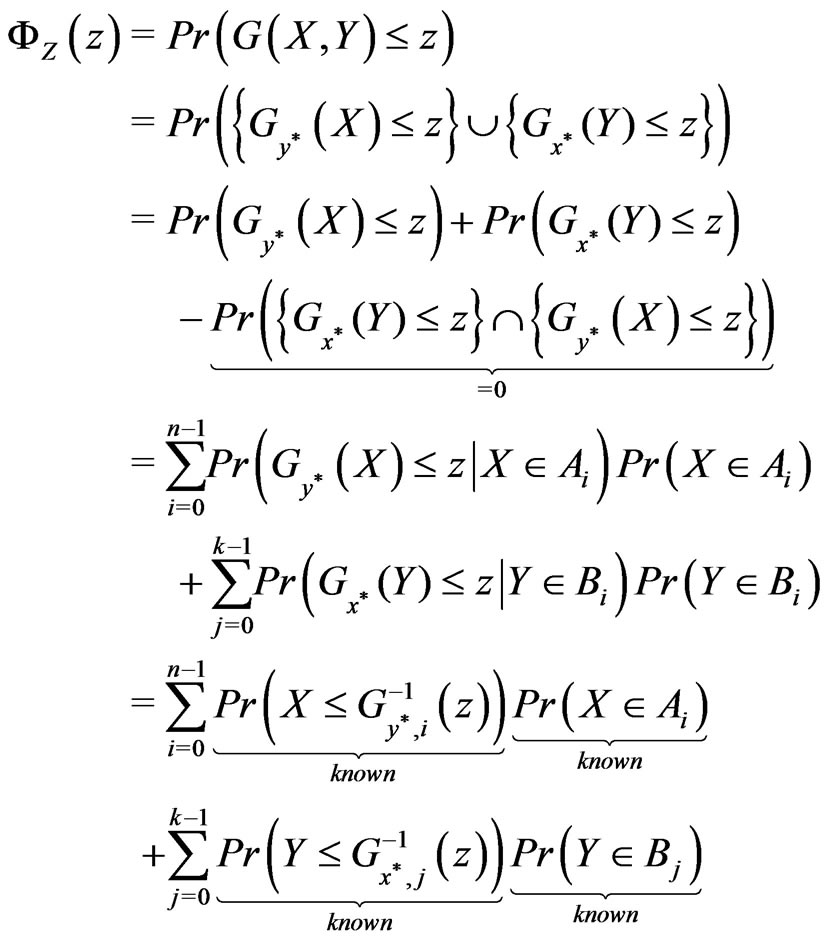
defines the cdf of  . Nicely, all of the above quantities can be computed since we specified the distributions for
  and
and . Note the zero quantity in the third line is due to the intersection of the sets containing only the single point
 . The
. The  and
and  depend on the length of
  and
and , respectively.
Similar to the 2D discrete setting, there is usually no closed form solution for  and thus
 , but the solution can be determined numerically. Figures 4(d)-(f) show the images from our technique applied to a simple two-dimensional discrete piecewise monotone function.
2.2.3. Extension to Larger Dimensions
In this manuscript, we directly show the calculations for one and two dimensions. However, our method can be extended to higher dimensions ( ) as demonstrated in [24].
2.3. Gaussian Noise Setting
In this section, we examine the properties of our procedure in light of Gaussian noise. In the 1D noise-free setting for image , it can be shown (with our proposed methods) that
  for any
  when
when  is the location of the absolute maximum, and
  when the sequence contained in each dimension of the smoothing window is monotone. Further, under certain circumstances associated with 1D images,
  when
when  is the location of a local minimum in our image; see [24] for details. The following examples, however, explore an
  image when noise is introduced in the raw image,
 . As expected, it will make spot detection in
  more difficult where the signal-to-noise will be important.
Consider adding independent and identically distributed (i.i.d.) Gaussian noise to the 1D monotonic sequence , where
 . Let
. Let , where
  denotes the true signal at location
 ,
,  equals the step size at
  in the monotonic sequence such that
 , and
, and  denotes normally distributed noise of mean zero and standard deviation
 . We fix
  for our examples such that the signal-to-noise ratio (
 ) remains constant within each simulation.
We examine the case when  at an arbitrary location
  since, as shown in [24], this may indicate a strictly increasing or decreasing sequence. In certain settings, a closed-form solution exists to compute the probability that the
  image is zero (
 ) over a monotone sequence with i.i.d. noise. In most cases, however, it is not possible to compute a closed-form solution for
 ; for notational simplicity, we use
  rather than
 . Figure 6 shows the empirical estimate for
  over a monotone sequence for different values of
  in the 1D situation. Note that the
  -axis is the ratio of stepsize to standard deviation of the noise, and that each curve begins at 1/(2c + 1) and asymptotes at 1. The signal-to-noise ratio,
  , is the critical value in evaluating how
  operates in a noisy environment. If the step size is 0, then each point in the window is equally likely to be the median, hence
 for any
  when
when . As the step size increases relative to the standard deviation of the noise, naturally for any
 , we expect the probability to converge to one. Hence, for noise-free monotone images,
  for all
 .
.
In the presence of noise, however, the monotone signal becomes contaminated such that  decreases as
  increases. Intuitively, as
  increases, the number of points in the smoothing window increases hence there are more “opportunities” for other points to be the median, thus making the residual nonzero at that location.
Given the local maximum at  in a noise-free 1D spot (mountain),
 . In the presence of noise, we can estimate (via simulation) the probability that the 1D residual image intensity value at the local maximum location is positive; i.e., we can estimate
  when
when  and
and

Figure 7(a) shows the estimated  at
at
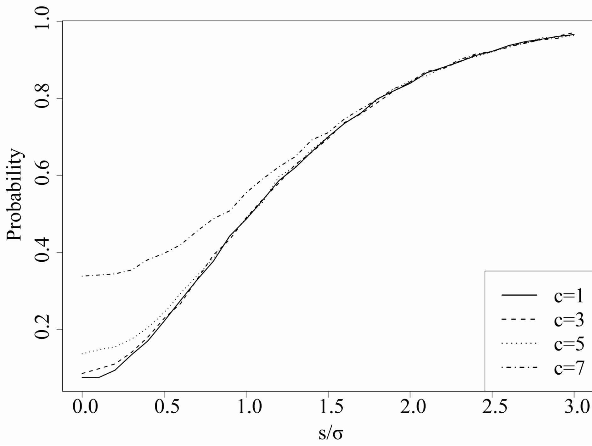
Figure 6. Estimated probability of R = 0: For different values of c (which indicate the size of the cross smoother), the y axis is the estimated probability that the R image is zero over a monotone signal of step size s contaminated with i.i.d. normally distributed noise with standard deviation 3/4. The x axis is the signal-to-noise ratio.

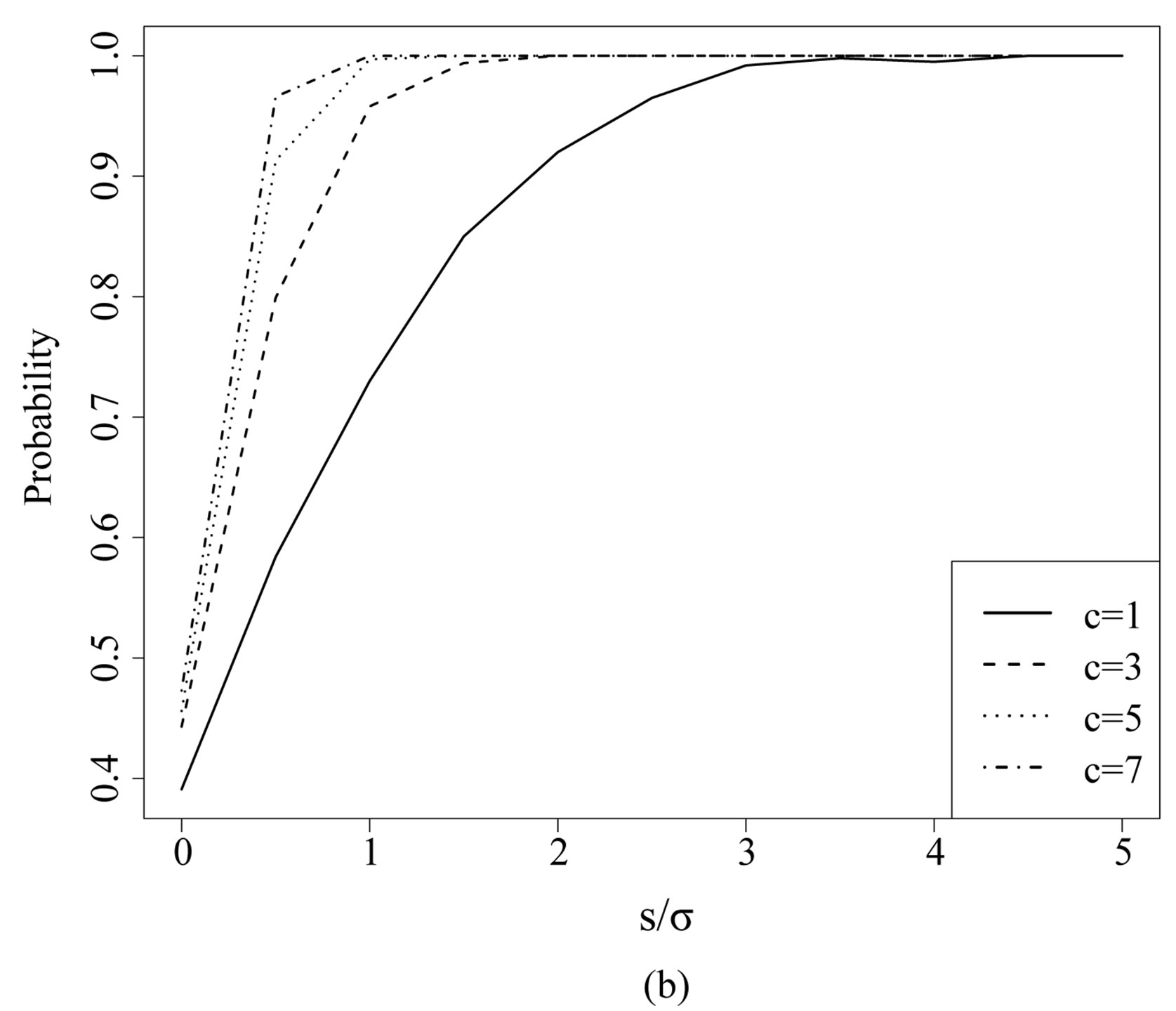
Figure 7. Estimated probability of R > 0 at a local maximum in 1D and 2D: (a) Pr(R1,c(p)) > 0, where p is the location of the absolute maximum in a 1D image; (b) Pr(R2; c(p1; p2)) > 0 for a 2D image, where (p1; p2) represents the location of the absolute maximum in the 2D image.
the absolute maximum location  as a function of
  for different values of
  in a 1D image. Analogously, Figure 7(b) shows
  for a maximum location
  when
when  is a 2D image. For all
 , the simulation results show that
  monotonically as the signal-tonoise ratio increases,
 . Further, as shown in Figures 7(a)-(b), as
  increases, the rate in which
  converges to 1 also increases, k = 1, 2.
To further illustrate the importance of the size of the smoothing window in detecting spots, Figures 8(a)-(b) shows a set of four Gaussian spots with different standard deviations. Figure 8(c) shows the  image resulting from the smoother being applied to Figure 8(a). Now, we add noise to the Gaussian spots shown in Figures 8(a)-(b) where the random (i.i.d) noise added at each pixel is distributed according to a Normal distribution with mean 0 and standard deviation 5, 15, or 50. Figures 9(a), (b), and (c) display the residual image when the smoother is applied to the Gaussian spots containing noise with standard deviations of 5, 15, or 50, respectively. With a fixed smoothing window, as the standard deviation of the noise increases, the ability to discern the cross decreases. Specifically at a standard deviation of 50, the crosses are nearly indistinguishable from noise for the top two mountains. Recall that, with the noise-free single mountain example, we clearly detected a cross in the rough operator image at the mountain’s maximum. Further, the size of the observed cross was directly related to the operating window. As the window size increased, the size of the cross increased as well. Consider adding noise to the mountain in Figure 4(d). Figure 10(a) shows a single mountain with i.i.d. N(0,
 ) noise added to the intensity at each pixel in Figure 4(d). Figures 10(b)-(c) show the associated
  images for a
  cross and a
  cross, respectively. There are several interesting features to note in this example. We see the respective crosses associated with the smoothing window; however, when using the
  arm, it is much harder to distinguish the cross from the remaining picture. With the
  arm, the cross is more apparent, mainly due to the cross being wider than in Figure 10(b).
To confirm that large values of c more effectively find spots, Figures 11(a)-(c) show a sequence of three spots in order of increasing size with  noise. Figures 11(d)-(f) are the R2,2 images corresponding to Figures 11(a)-(c), respectively. Figures 11(g)-(i) are the
  images corresponding to Figures 11(a)-(c). Figure 11 demonstrates two important results: (1) it is easier to

Figure 8. Bump hunting: (a) A 200 pixel × 200 pixel image consisting of four Gaussian spots with different locations and scales; (b) The associated perspective plot; (c) The “rough” residual image (R2,4 image) after running a specialized median smoother (s-median), S2,4. Crosses are present at the locations of their respective spot centers associated with the spots shown in (a).

Figure 9. Spot finding as noise increases: (a) R2,9 image associated with Figure 8, where i.i.d. normally distributed noise with mean 0 and standard deviation 5 (i.e. N(0, σ = 5)) was added to each pixel in Figure 8; (b) R2,9 image when the noise in Figure 8 is N(0, σ = 15); (c) R2,9 image when the noise in Figure 8 is N(0, σ = 50). As the standard deviation of the noise increases, the ability to detect the cross at each spot decreases.
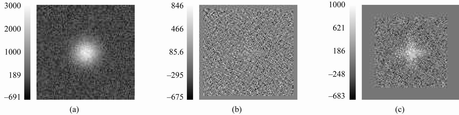
Figure 10. Mountains with noise added: (a) A 100 × 100 image of a 2D mountain where noise is normally distributed with 0 mean and standard deviation, 200; (b) The associated R2,9 image; the characteristic “cross” is difficult to discern by eye; (c) The R2,27 image; the characteristic “cross” is also difficult to detect because of the noise, however it is more detectable than the cross in (b).

Figure 11. Choice of smoothing operator: A series of Gaussian mountains of increasing size and N(0; σ = 48) noise are shown in (a), (b) and (c). The residual images R2,2 from applying an S2,2 operator to (a), (b), and (c) are shown in (d), (e), and (f), respectively. The residual images R2,3 from applying an S2,3 operator to (a), (b), and (c) are shown in (g), (h), and (i), respectively. The spots are more easily detected using the S2,3 operator (row 3) rather than the S2,2 operator (row 2).
detect larger spots in the presence of noise, and (2) in the presence of noise, larger values of c are more effective for detecting spots.
Collectively, Figures 6-11 illustrate the tradeoff that must be considered when determining the arm size for the s-median smoother. We see that large values of  are more likely to yield positive residuals at the maximum in the I image; however, the residuals associated with large values of c are also more likely to be nonzero in the presence of noise over monotonic regions. In other words, for spot finding, large values of c improve spot detection in noisy images, however, it may cause two distinct spots to merge into one spot in the presence of noise. A balance between these two issues will be critical in choosing the optimal c value(s) for peak or spot finding (see Section 3.4).
3. Results and Discussion
In this section, we present the results from applying our method to biologically motivated chemical sensor array data, including mass spectrometry, gel electrophoresis, and spotted microarray data. In mass spectrometry, the relevant data are represented as spectra where the associated peaks in the intensity plots represent proteins (or peptides) present in a sample. Obtaining the location and intensity of these peaks aides in identifying sample proteins for further study consideration. Gel electrophoresis data are represented in the form of 2D images comprised of protein spots. Again, investigators are interested in detecting these features in order to isolate their location in the image and potentially extract the associated protein sample for further analysis. Finally, spotted microarray data are represented as two-dimensional images of spots in a 2D matrix structure. Feature detection is key in order for the genetic data to be properly summarized and thus for these technologies to have utility in diagnosing disease or assessing putative biomarkers.
The code to perform our method is written using FIASCO, a collection of statistical software created in the Department of Statistics at Carnegie Mellon University that was originally designed to analyze functional magnetic resonance imaging (fMRI) data. The computer code used for this work are available upon request from the corresponding author. In the following, we demonstrate our spot detection technique on the various example sets noted above.
3.1. Mass Spectrometry
Matrix-assisted laser desorption ionization time-of-flight (MALDI-TOF) mass spectrometry is a technology that can be used to profile protein markers from tissue or bodily fluids, such as serum or plasma in order to compare biological samples from different patients or different conditions. The output from a MALDI-TOF experiment consists of a measured intensity for each massto-charge ratio (m/z) value; see Figure 12(a). The sets of expressed proteins are identified within each spectrum in order to ultimately determine differentially expressed proteins between conditions or samples. See [25] for further details describing the MALDI-TOF technology.
Our s-median derived  image can be used to detect peaks in MALDI-TOF images and thus locate peptides present in the sample. The spectrum for each sample consists of a single vector, I, thus applying the s-median is equivalent to applying a running median to the I image. This dataset in question was obtained from the Proteomics Core Laboratory at Roswell Park Cancer Institute. We use this real data to examine the results of applying the s-median to a MALDI-TOF spectrum. In this example, we set this dataset’s bandwidth (i.e. the value of
  in
in ) to 500 data points, which corresponds to approximately a 95 m/z bandwidth. Figure 12(b) shows the resulting s-median image using the chosen bandwidth; Figure 12(c) shows the associated
  image. From examining the R image, we note that the spikes in the original spectrum are preserved, thus aiding in the identification of the peak location. Further, the “negative peaks” in the residual image near the large spike serve to quantify the peak size in a MALDI-TOF image.
3.2. Gel Electrophoresis
Another application of this spot detection technique is on images obtained from two-dimensional difference gel electrophoresis (2D-DIGE) experiments such as those

Figure 12. Mass spectrometry: (a) MALDI spectrum based on a tumor sample; (b) S image based on a smoothing window of 95 m/z; (c) Associated R image that contains spikes at each local maximum in the original image I.
described in [26]. The ability to detect spots is crucial since missingness in this technology affects downstream analysis of detecting differential expression [27].
For our 2D-DIGE examples, we will focus on images representing portions of the 2D gels examining morphogenesis in Drosophila obtained from the Minden laboratory at Carnegie Mellon University [28,29]. These images are obtained from a charge-coupled device (CCD) camera and the protein spots in these images allow the researchers to obtain a protein expression signature of the sample under a given condition or given time point. The images under study have been normalized according to the model described in [26]. The full images are 1024  and densely populated with protein spots, making it difficult to observe individual protein spots in detail. We therefore focus on a
 sub-image to better understand the impact of applying the s-median.
Figure 13(a) shows the protein gel sub-image selected for illustration,  , with the associated perspective plot shown in Figure 13(b). Figure 13(c) displays the associated residual image,
 . From Figure 13(c), we can see the crosses associated with the protein spots shown in Figure 13(a). As well, we also see that each protein spot is outlined in black since, in the noise-free case, the
  image is negative at local minima in an image. Thus, we use the black outline as a boundary identification tool to determine spot size in order to more accurately determine summary information and excise the protein sample(s) of interest from the gel. In 2D-DIGE experiments, after quantification of the protein spots under different channels or conditions, similar to gene microarrays, the spot ratios are computed and compared to assess the degree of differential expression.
3.3. Spotted Microarrays
Genetic microarrays are a popular analysis tool to study genetic changes associated with diseases such as breast cancer [30]. The laser scanner images obtained from a microarray experiment consists of a series of spots indicating the measured fluorescence of a probe (or “gene”) deposited at that location. See [31] for a detailed description of the microarray technology, and [32] for an overview of the methods used for microarray analysis. Pin-based spotted microarrays have the probe material deposited on the glass slide via a microscopic pin tip. In the pin-tip based microarray technology, image analysis software is required to summarize the signal for a given spot on a chip. In this situation, we can examine the R image obtained from a pin microarray image for proper identification of spot locations and spots sizes to aid in spot quantitation and data summarization. Note that this technology can be extended to study proteins as in [33] and other biologically active molecules where antibodies can be developed and spotted to the chip and used as capture molecules. Thus, this technology has widespread potential as a chemical sensor panel to monitor biological activity (e.g., see [34-36]).
Figure 14(a) shows an example of a microarray image obtained from a cell cycle yeast experiment [37]. Similar to the gel electrophoresis example, Figure 14(b) examines a subsection of the microarray chip shown in Figure 14(a). Figure 14(c) shows the associated residual image ( ) obtained from applying an s-median to Figure 14(b). A closer inspection of Figure 14(c) reveals a black spot within the center of each microarray probe. This is an interesting phenomenon attributed to the manufacturing of the microarray. Occasionally, the impact of the pin onto the microarray chip displaces the probe material and causes a “doughnut” shape probe hybridization profile. The hybridization spot has a “hole” in the middle since there was little or no probe material deposited to hybridize. This effect is not obvious in Figure 14(b) but is clearly distinguished in Figure 14(c)- (d). This kind of information can be used to improve the estimation of spot intensity in the microarray image. The spot intensity estimates are used as input for downstream processing, ultimately, yielding the expression value for each probe representing the amount of hybridized genetic material.
3.4. Discussion
The classic equation,  , is well known to statisticians studying regression techniques or smoothing methods for datasets. In this manuscript, we demonstrate an application of this equation, resulting in a new operator where the residual image derived from a novel smoother can be used to locate spots or mountains in an image. This method combines the residual operator from statistics with the structuring element (cross-shaped window) in the field of mathematical morphology. Major advantages of our method include fast running time, broad application to many image types, and universal spot detection regardless of scale. That is, irrespective of a spot’s size and height, its location will be detected via our method. This aspect alleviates the need to alter or change the grey scales in an image when searching for spots of varying intensities.
As demonstrated, this method uses the s-median operator to smooth images. Other window operators can be considered, however they result in different residual image implications. For example, if a mean cross (i.e. “smean”) smoother is used on the Gaussian mountain in Figure 15(a) rather than a median smoother, the residual image does not reveal the shape of the mountain; see, e.g., Figure 15(b). Further, the shape of the smoothing window is also a critical component of consideration. Figure 15(c) displays the results when a median smoother with a

Figure 13. 2D-DIGE images: (a) Subset of 2D-DIGE image. This 50 pixel × 50 pixel image is a subimage of the Drosophilia proteome gel, normalized according to the model in [26]; (b) The associated perspective plot for the data in (a); (c) The associated R2,6 image. There are several “crosses” apparent, which indicate protein spots in the image. There is also a “speckled” black and white noise pattern present in the image with a black outline around several of the spots.

Figure 14. Gene microarray: (a) Full image of a microarray chip containing roughly 4000 spots; (b) Microarray subimage showing roughly 25 spots; (c) R2,4 image resulting from the s-median smoother applied to (b). Note the black pixels at the center of each spot indicate local minima. Common phenomena of pin microarray images are local minima due to the lack of probe material caused by the pin containing the probe material impacting against the glass slide. This impact causes a “donut” pattern in the perspective plot of the microarray image. This donut pattern is clearly recognized in (c); (d) A perspective plot of the data shown in (c) further detailing the donut pattern.

Figure 15. Other measures: The results from different variations on the s-median. (a) A Gaussian spot image, I, of dimension 50 × 50; (b) The R2,2 image obtained from using an s-mean rather than s-median on the image in (a); (c) Associated residual image obtained from (a) using an s-median, where the window sequence is a 5 pixel × 5 pixel box shape containing all 25 pixels.
grid or “box” shaped window sequence is used. Here, we now obtain a residual image that looks like a starburst instead of a cross. As a result, the spot center is now potentially more difficult to identify. The shape of the smoothing window (cross vs. box) and the summary statistic used (median versus mean) thus affect the R image and the ability to detect the mountains in an image.
The issue of rotation invariance is an important concept within mathematical morphology operators used in image detection. Rotation invariance implies that the resultant image does not change when arbitrary rotations are applied to its input argument. In general, our spot finding method is rotation invariant for the Gaussian spots with zero correlation (e.g., spots of the type shown in Figure 8). Interestingly, if we induce any nonzero correlation in the spot, the spot finding method is no longer rotation invariant. Figure 16(a) displays a bivariate normal density with a correlation of 0.50 between the two variables. Figure 16(b) is the residual image from our proposed method. Meanwhile, Figure 16(c) is the result when employing a rotated version (45 degrees) of the structuring element used in Figure 16(b). Similarly, Figure 16(d) is the rotated version (90 degree) of Figure 16(a) with the corresponding  images shown in Figures 16(e)-(f). Our proposed spot finding method is not rotation invariant since the images in Figure 16(b) and Figure 16(e) are clearly different. Although our proposed method is not rotation invariant, it is possible to rotate our structuring element (cross) to align with the major and minor axes of a correlated spot as in Figures 16(c) and (f). Both versions of the residual images clearly show a cross shape and provide utility in terms of locating the spots in the image. Future work will further explore the characteristics of the cross in each residual image in order to detect spots in correlated images. Note, however, in our biological applications (e.g. 2D-DIGE), it is reasonable to assume that there is negligible correlation within a spot. For example in a DIGE image, the spots are created by electrophoresis in two dimensions where the electrophoresis for each dimension is performed separately. Similarly in pin-based microarray images, it is reasonable to assume that there is negligible correlation within a given spot.
When using the s-median operator for spot finding, the major consideration is the arm-length size  associated with the smoothing window, or alternatively the number of pixels included in the smoothing window (structuring element). The s-median smoother naturally removes noise from
 , hence the size of the smoothing window essentially decides the amount of smoothing to apply to the dataset. From Figures 11 and 17, the choice of
  is critical, since choosing
  too large will oversmooth the image and blend spots together, while choosing
  too small will undersmooth the image and cause spurious spots due to noise to appear as real spots. Since the choice of
  is essentially choosing a smoothing parameter, there are several available methods to consider when choosing an optimal value for c. The general method for choosing smoothing parameters is based on cross validation algorithms described in [22].
The optimal choice of c is related to the larger statistical subject of bias-variance tradeoff. Choosing c too small leads to a largely variable residual image (missing small spots), while choosing c too large leads to a residual image with a large bias term (too many spurious spots). Similarly, the optimal choice of c is related to several other problems in statistics, the optimal choice of bandwidth in kernel density estimation [38], and the amount of times to smooth a dataset [39]. Various strategies that estimate error quantities (risk) can determine “optimal” smoothing strategies, while other procedures determine smoothing parameters from examining figures such as mode trees [40] or estimates of the mean squared error [41]. To improve the ability of our MM operator in the presence of noise, we have explored applying standard image smoothing techniques to the image prior to applying the MM filter. Future work will examine the utility of applying “pre-smoothers” to images before applying MM operators. In addition to examining pre-smoothers, we will also examine data driven cross validation schemes for choosing an optimal value of c for specific image applications. In the same way we use presmoothers to smooth the image prior to analysis, we will also explore smoothing the resulting residual image.
A major concern in proposing image analysis software algorithms involves performing the comparisons among competing methods. Unfortunately, due to the cost of these technologies and the lack of a gold standard for measuring the signal of the chemical sensor, it is difficult to design statistically appropriate benchmarks or quality control studies to assess these image analysis techniques for a given chemical sensor. Although it is relatively simple to simulate “bumps” or mountains in an image, the difficulty arises in deciding the type of noise to impose upon the simulated images. In the presence of most noise distributions, the success of our proposed method will be dependent on the choice of smoothing parameter, c. It is outside the scope of this manuscript to perform a thorough comparison of competing spot finding algorithms against a set of noise distributions. For future work, we propose performing comparisons such as those in [42, 43] to establish conditions in simulated and real datasets where our methods are superior to competing methods. The main goal of this manuscript is to establish a new method for spot finding in images and demonstrate its performance on a variety of different biological images derived from chemical sensors.

Figure 16. Rotational invariance: (a) A scaled bivariate normal density with a correlation of 0.50; (b) The resulting residual image using a R2,4 operator; (c) The resulting residual image when the structuring element in the residual operator used in (b) is rotated 45 degrees to align with the major axis of the spot in (a); (d) a 90 degree rotation of the spot in (a), i.e. a spot with a correlation of –0.50; (e) The residual image using a R2,4 operator. The resulting residual image when the structuring element used in (e) is rotated 45 degrees.
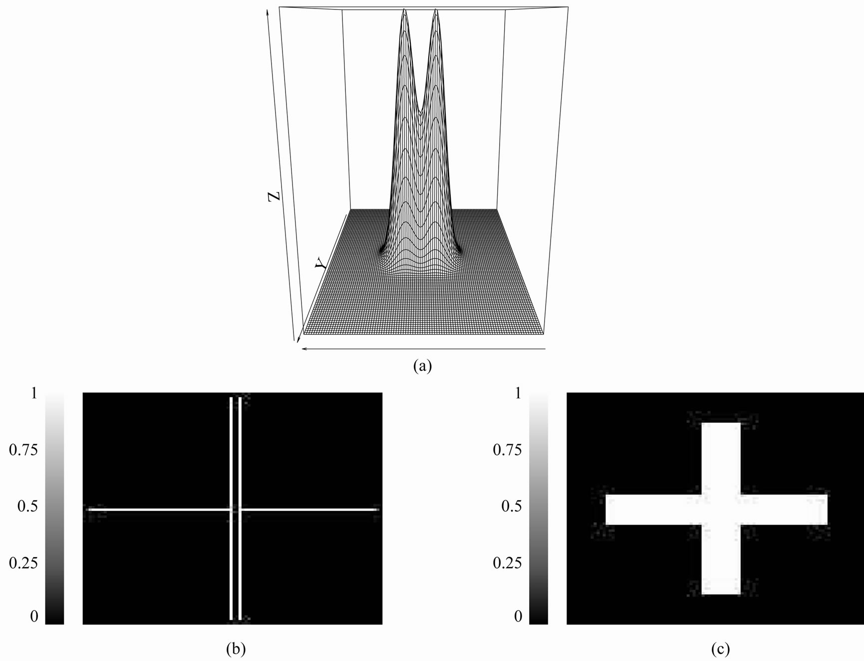
Figure 17. Two nearby mountains: (a) Perspective plot showing two relatively close mountains; (b) The R2,5 operator image associated with the image in (a). The two crosses indicate the presence of two relative maxima in the image; (c) The R2,27 image obtained from the image in (a). In this situation, the two mountains are “blurred” into one cross.
4. Conclusion
This manuscript develops a new method for spot finding and illustrates the technique’s great utility and applicability within several chemical sensor datasets such as mass spectrometry spectra, gel electrophoresis images, and microarray images. This method can be easily extended to mountains in k dimensions and can be extended to further quantify the amount of signal present in other emerging chemical sensors with Gaussian profiles.
5. Acknowledgements
The authors are grateful to the Roswell Park Cancer Institute Proteomics laboratory and the Minden laboratory at Carnegie Mellon University for generously providing their data to illustrate our method. We also thank the reviewers of this manuscript for their valuable feedback and insights.
REFERENCES
- D. Agard, R. Steinberg, and R. Stroud, “Quantitative Analysis of Electrophoretograms: A Mathematical Approach to Super-Resolution,” Analytical Biochemistry, Vol. 111, No. 2, 1981, pp. 257-268. doi:10.1016/0003-2697(81)90562-5
- E. Bertin and S. Arnouts, “Sextractor: Software for Source Extraction,” Astronomy and Astrophysics, Vol. 14, No. 4, 1996.
- T. Lindeberg, “Feature Detection with Automatic Scale Selection,” International Journal of Computer Vision, Vol. 30, No. 2, 1998, pp. 79-116. doi:10.1023/A:1008045108935
- K. Coombes, H. Fritsche Jr., C. Clarke, J. Chen, K. Baggerly, J. Morris, L. Xiao, M. Hung and H. Kuerer, “Quality Control and Peak Finding for Proteomics Data Collected from Nipple Aspirate Fluid by Surface-Enhanced Laser Desorption and Ionization,” Clinical Chemistry, Vol. 49, No. 10, 2003, pp. 1615-1623. doi:10.1373/49.10.1615
- P. Cutler, G. Heald, I. R. White and J. Ruan, “A Novel Approach to Spot Detection for Two-Dimensional Gel Electrohporesis Images Using Pixel Value Collection,” Proteomics, Vol. 3, No. 4, 2003, pp. 392-401. doi:10.1002/pmic.200390054
- D. S. Lalush, “Effects of Spot and Background Defects on Quantitative Data from Spotted Microarrays,” Proceedings of the 25th Annual International Conference of the IEEE, Vol. 4, 2003, pp. 3563-3566.
- K. Coombes, S. Tsavachidis, J. Morris, K. Baggerly, M. Hung and H. Kuerer, “Improved Peak Detection and Quantification of Mass Spectrometry Data Acquired from Surface-Enhanced Laser Desorption and Ionization by Denoising Spectra with the Undecimated Discrete Wavelet Transform,” Proteomics, Vol. 5, No. 16, 2005, pp. 4107-4117. doi:10.1002/pmic.200401261
- A. Jain and D. Zongker, “Feature Selection: Evaluation, Application, and Small Sample Performance,” IEEE Transactions on Pattern Analysis and Machine Intelligence, Vol. 19, No. 2, 1997, pp. 153-158. doi:10.1109/34.574797
- B. Guo, R. Damper, S. Gunn and J. Nelson, “A Fast Separability-Based Feature-Selection Method for HighDimensional Remotely Sensed Image Classification,” Pattern Recognition, Vol. 41, No. 5, 2008, pp. 1653-1662. doi:10.1016/j.patcog.2007.11.007
- J. Serra, “Image Analysis and Mathematical Morphology 1982,” Academic Press, New York, 1986, pp. 370-382.
- P. Maragos, “Tutorial on Advances in Morphological Image Processing and Analysis,” Optical Engineering, Vol. 26, No. 7, 1987, pp. 623-632.
- P. Maragos and R. Schafer, “Morphological Filters Part I: Their Set-Theoretic Analysis and Relations to Linear Shift-Invariant Filters,” IEEE Transactions on Acoustics, Speech and Signal Processing, Vol. 35, No. 8, 1987, pp. 1153-1169.
- P. Maragos and R. Schafer, “Morphological Filters Part II: Their Relations to Median, Order-Statistic, and Stack Filters,” IEEE Transactions on Acoustics, Speech and Signal Processing, Vol. 35, No. 8, 1987, pp. 1170-1184. doi:10.1109/TASSP.1987.1165254
- P. Maragos, R. Schafer and M. Butt, “Mathematical Morphology and Its Applications to Image and Signal Processing,” Springer, New York, 1996. doi:10.1007/978-1-4613-0469-2
- P. Soille, “Morphological Image Analysis: Principles and Applications,” Springer-Verlag, New York, 2003.
- D. Gavrila, J. Giebel, M. Perception, D. Res and G. Ulm, “Shape-Based Pedestrian Detection and Tracking,” IEEE Intelligent Vehicle Symposium, Vol. 1, 2002, pp. 8-14.
- L. Tarassenko, P. Hayton, N. Cerneaz and M. Brady, “Novelty Detection for the Identification of Masses in Mammograms,” Fourth International Conference on Artificial Neural Networks, Cambridge, 26-28 June 1995, pp. 442-447.
- E. Saber and A. Murat Tekalp, “Frontalview Facedetection and Facial Feature Extraction Using Color, Shape and Symmetry Based Cost Functions,” Pattern Recognition Letters, Vol. 19, No. 8, 1998, pp. 669-680. doi:10.1016/S0167-8655(98)00044-0
- Y. Wang, C. Chua and Y. Ho, “Facial Feature Detection and Face Recognition from 2D and 3D Images,” Pattern Recognition Letters, Vol. 23, No. 10, 2002, pp. 1191- 1202. doi:10.1016/S0167-8655(02)00066-1
- E. Lehmann and G. Casella, “Theory of Point Estimation,” Springer, New York, 1998.
- T. Apostol and I. Makai, “Mathematical Analysis,” Addison-Wesley, Reading, 1974.
- L. Wasserman, “All of Statistics: A Concise Course in Statistical Inference,” Springer, New York, 2004.
- G. Casella and R. L. Berger, “Statistical Inference,” Duxbury Press, Belmont, 1990.
- J. Miecznikowski, K. Sellers and W. Eddy, “Multidemensional Median Filters for Finding Bumps,” Technical Report 907, SUNY University at Buffalo, Buffalo, 2009.
- M. Karas, U. Bahr, A. Ingendoh, E. Nordhoff, B. Stahl, K. Strupat and F. Hillenkamp, “Principles and Applications of Matrix-Assisted UV-Laser Desorption/Ionization Mass Spectrometry,” Analytica Chimica Acta, Vol. 241, No. 2, 1990, pp. 175-185. doi:10.1016/S0003-2670(00)83645-4
- K. Sellers, J. Miecznikowski, S. Viswanathan, J. Minden and W. Eddy, “Lights, Camera, Action: Quantitative Analysis of Systematic Variation in Two-Dimensional Difference Gel Electrophoresis,” Electrophoresis, Vol. 28, No. 18, 2007, pp. 3324-3332. doi:10.1002/elps.200600793
- J. Miecznikowski, S. Damodaran, K. Sellers, D. Coling, R. Salvi and R. Rabin, “A Comparison of Imputation Procedures and Statistical Tests for the Analysis of TwoDimensional Electrophoresis Data,” Proteome Science, Vol. 9, No. 14, 2011, p. 66.
- J. Mergliano and J. Minden, “Caspase-Independent Cell Engulfment Mirrors Cell Death Pattern in Drosophila Embryos,” Development, Vol. 130, No. 23, 2003, pp. 5779- 5789. doi:10.1242/dev.00824
- L. Gong, M. Puri, M. Unlu, M. Young, K. Robertson, S. Viswanathan, A. Krishnaswamy, S. Dowd and J. Minden, “Drosophila Ventral Furrow Morphogenesis: A Proteomic Analysis,” Development, Vol. 131, No. 3, 2004, pp. 643-656. doi:10.1242/dev.00955
- J. Miecznikowski, D. Wang, S. Liu, L. Sucheston and D. Gold, “Comparative Survival Analysis of Breast Cancer Microarray Studies Identifies Important Prognostic Genetic Pathways,” BMC Cancer, Vol. 10, No. 1, 2010, p. 573. doi:10.1186/1471-2407-10-573
- M. Schena, D. Shalon, R. Davis and P. Brown, “Quantitative Monitoring of Gene Expression Patterns with a Complementary DNA Microarray,” Science, Vol. 270, No. 5235, 1995, pp. 467-470. doi:10.1126/science.270.5235.467
- R. Gentleman, “Bioinformatics and Computational Biology Solutions Using R and Bioconductor,” Springer, New York, 2005. doi:10.1007/0-387-29362-0
- C. Schröder, A. Jacob, S. Tonack, T. Radon, M. Sill, M. Zucknick, S. Rüffer, E. Costello, J. Neoptolemos, T. Crnogorac-Jurcevic, et al., “Dual-Color Proteomic Profiling of Complex Samples with a Microarray of 810 Cancer-Related Antibodies,” Molecular & Cellular Proteomics, Vol. 9, No. 6, 2010, pp. 1271-1280. doi:10.1074/mcp.M900419-MCP200
- M. Eisen, P. Spellman, P. Brown and D. Botstein, “Cluster Analysis and Display of Genomewide Expression Patterns,” Proceedings of the National Academy of Sciences, Vol. 95, No. 25, 1998, pp. 14863-14868. doi:10.1073/pnas.95.25.14863
- A. Alizadeh, M. Eisen, R. Davis, C. Ma, I. Lossos, A. Rosenwald, J. Boldrick, H. Sabet, T. Tran, X. Yu, et al., “Distinct Types of Diffuse Large b-Cell Lymphoma Identified by Gene Expression Profiling,” Nature, Vol. 403, No. 6769, 2000, pp. 503-511. doi:10.1038/35000501
- J. Khan, J. Wei, M. Ringnér, L. Saal, M. Ladanyi, F. Westermann, F. Berthold, M. Schwab, C. Antonescu, C. Peterson, et al., “Classification and Diagnostic Prediction of Cancers Using Gene Expression Profiling and Artificial Neural Networks,” Nature Medicine, Vol. 7, No. 6, 2001, pp. 673-679. doi:10.1038/89044
- G. Fink, P. Spellman, G. Sherlock, M. Zhang, V. Iyer, K. Anders, M. Eisen, P. Brown, D. Botstein and B. Futcher, “Comprehensive Identification of Cell Cycle-Regulated Genes of the Yeast Saccharomyces Cerevisiae by Microarray Hybridization,” Molecular Biology of the Cell, Vol. 9, No. 12, 1998, pp. 3273-3297.
- B. Silverman, “Density Estimation for Statistics and Data Analysis,” Chapman & Hall/CRC, 1986.
- J. Tukey, “Exploratory Data Analysis,” Addison-Wesley, New York, 1977.
- M. Minnotte and D. Scott, “The Mode Tree: A Tool for Visualization of Nonparametric Density Features,” Journal of Computational and Graphical Statistics, Vol. 2, No. 1, 1993, pp. 51-68. doi:10.2307/1390955
- J. Miecznikowski, D. Wang and A. Hutson, “Bootstrap Mise Estimators to Obtain Bandwidth for Kernel Density Estimation,” Communications in Statistics Simulation and Computation, Vol. 39, No. 7, 2010, pp. 1455-1469. doi:10.1080/03610918.2010.500108
- Y. Kang, T. Techanukul, A. Mantalaris and J. Nagy, “Comparison of Three Commercially Available DIGE Analysis Software Packages: Minimal User Intervention in Gel-Based Proteomics,” Journal of Proteome Research, Vol. 8, No. 2, 2009, pp. 1077-1084. doi:10.1021/pr800588f
- Y. Chao, H. Zengyou and Y. Weichuan, “Comparison of Public Peak Detection Algorithms for Maldi Mass Spectrometry Data Analysis,” BMC Bioinformatics, Vol. 10, No. 4, 2009.