Journal of Transportation Technologies
Vol.08 No.03(2018), Article ID:86077,23 pages
10.4236/jtts.2018.83012
Resource Efficient Hardware Implementation for Real-Time Traffic Sign Recognition
Huai-Mao Weng, Ching-Te Chiu
Department of Electrical Engineering, National Tsing-Hua University, Taiwan

Copyright © 2018 by authors and Scientific Research Publishing Inc.
This work is licensed under the Creative Commons Attribution International License (CC BY 4.0).
http://creativecommons.org/licenses/by/4.0/


Received: May 22, 2018; Accepted: July 17, 2018; Published: July 20, 2018
ABSTRACT
Traffic sign recognition (TSR, or Road Sign Recognition, RSR) is one of the Advanced Driver Assistance System (ADAS) devices in modern cars. To concern the most important issues, which are real-time and resource efficiency, we propose a high efficiency hardware implementation for TSR. We divide the TSR procedure into two stages, detection and recognition. In the detection stage, under the assumption that most German traffic signs have red or blue colors with circle, triangle or rectangle shapes, we use Normalized RGB color transform and Single-Pass Connected Component Labeling (CCL) to find the potential traffic signs efficiently. For Single-Pass CCL, our contribution is to eliminate the “merge-stack” operations by recording connected relations of region in the scan phase and updating the labels in the iterating phase. In the recognition stage, the Histogram of Oriented Gradient (HOG) is used to generate the descriptor of the signs, and we classify the signs with Support Vector Machine (SVM). In the HOG module, we analyze the required minimum bits under different recognition rate. The proposed method achieves 96.61% detection rate and 90.85% recognition rate while testing with the GTSDB dataset. Our hardware implementation reduces the storage of CCL and simplifies the HOG computation. Main CCL storage size is reduced by 20% comparing to the most advanced design under typical condition. By using TSMC 90 nm technology, the proposed design operates at 105 MHz clock rate and processes in 135 fps with the image size of 1360 × 800. The chip size is about 1 mm2 and the power consumption is close to 8 mW. Therefore, this work is resource efficient and achieves real-time requirement.
Keywords:
Traffic Sign Recognition, Advanced Driver Assistance System, Real-Time Processing, Color Segmentation, Connected Component Analysis, Histogram of Oriented Gradient, Support Vector Machine, German Traffic Sign Detection Benchmark, CMOS, ASIC, VLSI

1. Introduction
Driver Assistance System (ADAS) is a common device in modern cars. ADAS is designed to enhance car safety and driving comfort. ADAS often includes automotive navigation, autonomous cruise control, collision avoidance, lane departure warning, and so on. The Traffic Sign Recognition (TSR, or Road Sign Recognition, RSR) can help driver notice the fast passed signs, thus avoiding traffic violations or accidents. The TSR must be fast enough to react to the changing traffic conditions. The recognition rate of TSR should be high enough to detect most signs and prevent false information. The method should be fast as well as easy to implement with hardware, which is able to process in real-time. Besides, a well-designed hardware implementation should be energy saving as well as low cost, which means resource efficiency.
There are many researches for TSR proposed. Mammeri et al. [1] classify the most traffic sign recognition methods into three categories, which are image-processing (traditional computer-vision) based, machine learning based and hybrid method. The image-processing based methods use various ComputerVision techniques to find traffic signs in the source image. Gomez-Moreno et al. [2] make a comparison of several color segmentation methods for TSR, and shows that the RGB Normalized method performs the best result. Khan et al. [3] use the Gabor filter and the K-mean clustering to segment the signs. Ming Liang et al. [4] perform a SVM-based color transform. Liang et al. [4] use the template matching method with templates of different orientations. The shape analysis proposed by Khan et al. [3] verifies the basic polygon properties of the signs. Gonzalez et al. [5] propose a VISUALISE system, which implements the constrained Hough transform to extract the edge of signs in the luminance image. Most image-processing based methods are simple to implement and the computing speed is fast. However, the recognition rate is relatively low.
The machine learning (ML) based method has been used in the traffic sign recognition recently. The descriptor and classifier method is one of the ML techniques. Overett et al. [6] propose a LiteHOG+ descriptor that extended the HOG feature [7] by a centre-surround statistics, and classify with a cascade FDA classifier. Seo et al. [8] present a color-based feature with AdaBoost classifier to detect the signs. Besides, they construct a log-polar transform and the SVM method to classify the signs. Another common ML technique is the artificial neural network. Zhang et al. [9] propose the probabilistic neural network to recognize traffic signs. Jin et al. [10] construct the convolutional neural networks and train with a hinge loss stochastic gradient descent method. The ML based method achieves high recognition rate. However, the massive computational complexity makes it difficult to process in real-time with appropriate computing resources.
The hybrid method divides the TSR procedure into two stages, detection and recognition. The detection stage use the image-processing based method to detect the potential signs in the source image. The recognition stage uses the machine learning based method to recognize the detected signs. Thus, the hybrid method takes both advantages of fast computation and high recognition rate. There are various techniques in the detection stage. A specialized color transform with thresholding, followed by the Connected Component Labeling (CCL) procedure, is an effective way to extract traffic signs [11] [12] [13] . Some researches [14] [15] [16] use the maximally stable extremal region (MSER) to extract the stable regions. Liu et al. [17] propose the High-Contrast Region Extraction to extract the regions by a possibility map. In the recognition stage, the descriptor and classifier method is often used. The common descriptor choices are the Histogram of Oriented Gradient (HOG) [4] [12] [13] [14] [16] or modified HOG [6] , [15] . The classifier can be support vector machine (SVM) [5] [12] [13] [14] [15] , neural networks [16] or SRC-based classifier [17] . Most of the recently propose researches implement the hybrid method, so does this work.
We propose a high efficient TSR method, which reaches high recognition rate and processes in real-time. Our contribution is to propose an efficient two-phase method to eliminate the “merge-stack” operations so the operation speed and memory cost in the CCL module is significantly improved. The method achieves 96.61% detection rate and 90.85% recognition rate while testing with GTSDB dataset. The proposed TSR method is further implemented on hardware. The hardware implementation aims to reduce the storage and simplify the computation of software implementation. By using TSMC 90 nm process, the proposed hardware operates at 105 MHz clock frequency and processes 135 fps with the image size of 1360 × 800. The proposed TSR method is illustrated in Section 2. Section 3 shows the performance evaluation results and the testing method we used. Section 4 introduces the hardware architecture of the proposed method and shows the tap-out results. A brief conclusion is given in Section 5.
2. Proposed TSR Method
We propose the hybrid traffic sign recognition method. The method contains two main stages, detection and recognition. In the detection stage, we use Normalized RGB color transform and Single-Pass Connected Component Labeling (CCL) to find the potential traffic signs. In the recognition stage, Histogram of Oriented Gradient (HOG) is used to generate the descriptor of the signs, and we classify the signs with Support Vector Machine (SVM). The overall flow chart of main TSR procedures is shown in Figure 1. We describe the procedures in detail in the following subsections.
2.1. Detection Procedure
The detection procedure is used to detect the potential traffic signs form the source image. It is the most time consumption part of the whole TSR procedure. Because we have to scan the whole source image to find the potential traffic signs Figure 2. Results of each step in the detection procedure (or Region-of-Interest, ROI) before recognizing every found ROIs. Figure 2 shows the results of each step in the detection procedure.

Figure 1. Flow chart of the proposed TSR method. The left side shows the detection procedure, and the right side shows the recognition.

Figure 2. Result of each step in the detection procedure. (a) Example extracted from the source image (full color); (b) NRB color transform (gray-scale image produced); (c) Multiple thresholding (3 binary images produced); (d) Single-pass connected component labeling (ROIs extracted).
1) Reducing the Searching Space: Fortunately, the traffic signs do not appear at any location of the source image. For example, the signs do not appear at the sky and surface. Therefore, we are able to reduce the searching space by removing the top and the bottom of source images. In addition, we split a source image into left-frame and right-frame, then process two frames independently. Figure 3 shows the layout of the frames. Our experiment shows that there are less than 4% of total signs are out of the searching space. On the other hand, because the

Figure 3. Searching space and the layout of two frames in the source image.
images are taken from the moving car, the out-of-space signs will move into the searching space over time.
2) Color Segmentation: We use the color segmentation to extract the specified color of the traffic sign boundary, e.g. red and blue. The color segmentation contains two parts. The first part is the color transform. The researches [5] [14] [15] claim that the Normalized-RGB Color Transform performs the most robust result under different lighting and contrast condition. A gray-scale image is generated by the color transform, and the value is higher for red or blue, lower for other colors. We emphasize the negative influence of green color, in other words, a pixel that has greener ingredient is less likely to be the targeted blue or red color. The modified normalized RGB color transform, called NRB color transform, is shown as following:
(1)
where R, G, B are the red, green and blue color channel, respectively. max(R; B) is the maximum value between R and B. α is a small constant, we set to 8. β is a green color magnification, we set to 4 in this work.
The second part is the thresholding. A threshold is used to determine if the pixel has the specified color or not. The transformed pixel that passes the threshold will be set to 1, otherwise 0. Thus, the binary image is produced by the color segmentation. For the flexibility under different conditions, we use multiple thresholds instead of a single threshold. Hence, multiple binary images are produced by thresholding.
3) Single-Pass Connected Component Labeling: We use the Connected Component Labeling (CCL) algorithm to group the white pixels in the binary image. The CCL algorithm scans the binary image and assigns the label to each pixel using only local operations [18] . A set of connected pixels is called a “region”. As shown in Figure 4, two pixels are “connected” if they are adjacent to each other. The traditional two-pass CCL algorithm produces the labeled image, where all pixels that belong to a region are labeled to the same number. The first pass of CCL is to scan the pixels and record the connecting relations. The initially labeled image is generated, but the label number may be incorrect because there
 (a)
(a)
 (b)
(b)
Figure 4. The adjacent pixels of (a) 4-connectivity; (b) 8-connectivity. The central pixel is marked as × and the adjacent pixels are gray. The pixels with letters are the ones that should be checked while scanning the image.
are unread pixels when scanning the image in the first pass. Hence, the second pass is to re-label the incorrect labels by the recorded relations.
Obviously, the connecting relations of the pixels are built in the first pass, while the second pass is only used to replace the incorrect labels in the labeled image. Abubaker et al. [19] propose the single-pass algorithm for the connected component analysis. If we do not need the labeled image as the result, the second pass can be eliminated. Instead, we extract some “features” of the regions during the first pass. Because of the elimination of the second pass, the theoretical computing time of the single-pass algorithm is half comparing to the two-pass algorithm.
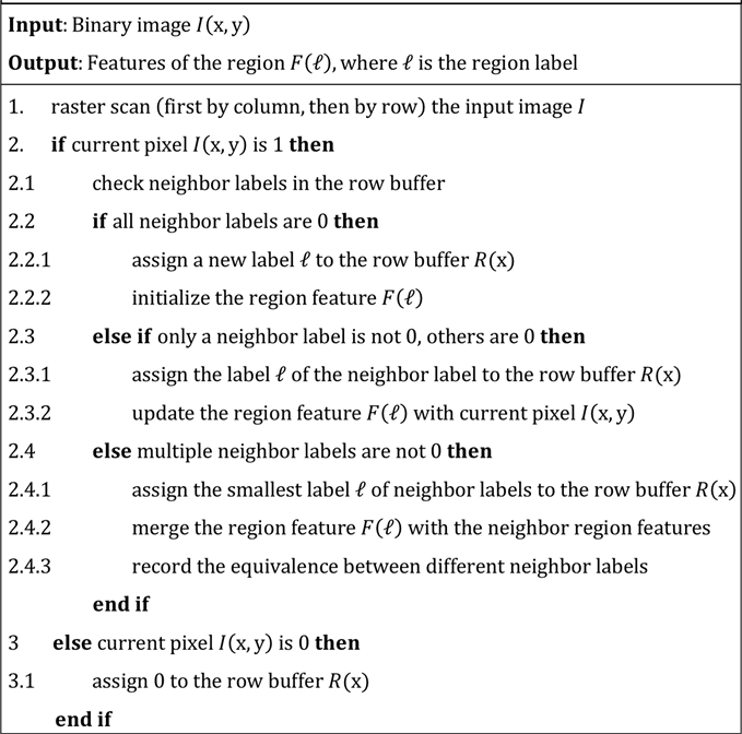
Furthermore, the memory requirement is reduced. According to Figure 4, when we scan the pixels in the binary image, the decision of the current label number is observed by only the neighbor labels in the previous row. Because the result is features of the region, the completely labeled image can be replaced by a labeled row, called the “row-buffer”. Besides, the “data-table” is introduced to store the extracted region features. Overall, the total memory of the CCL is greatly reduced by the elimination of labeled image, even though the additional storage, e.g. the data-table, is required. The main procedure of single-pass CCL algorithm can be expressed as the pseudo code of Algorithm 1. We select the bounding box as the region feature in this work. The bounding box contains the boundaries of regions, which lets us extract the ROIs from the source image. Finally, we can pass the detected ROIs to the next main procedure, recognition.
2.2. Recognition Procedure
The recognition procedure is used to classify the potential traffic signs found by the detection procedure. Besides, there are many false detected ROIs, which should be removed. The schematic diagram of the recognition procedure is shown in Figure 5. We first check the region criteria. It can be done by observing only the bounding box information. The width and height of the region should not be greater than 110% of the maximal size nor less than 90% of the minimal size. The width/height ratio should be within 0.75 and 1.25. According to the experiment, there are averagely 10.75 ROIs per image that meet the criteria. We extract the eligible regions from the source image. They are converted into gray-scale and resized to 32 × 32, before the HOG calculation.

Figure 5. Schematic diagram of the recognition procedure. (a) ROI boundaries produced by detection procedure; (b) Extracted traffic signs; (c) Resize and convert to gray-scale; (d) HOG descriptor calculation; (e) SVM classification; (f) Traffic sign recognized.
Algorithm 1. Single-pass connected components labeling.
1) Simplification of HOG Calculation: Next, we calculate the HOG descriptor of the regions. We choose the HOG parameters that reference to N. Dalal et al. [7] : 3 × 3 blocks per window, 2 × 2 cells per block, 8 × 8 pixels per cell, an 8-bin histogram spreads over 0 to 360 degrees, and the arithmetic mean is used for normalization. Not all parameters are same as the original research. Moreover, we replace the floating-point calculation with fixed-point for simplification and faster computation. In other words, the quantization is performed for easier hardware implementation.
We use some approximate formulas instead of the original precise formulas. The gradient calculation of X-axis and Y-axis are:
(2)
which are same as the original ones. We use the Manhattan distance to approximate the magnitude calculation:
(3)
where |gradx| and |grady| are the absolute values of X-gradient and Y-gradient. When we need only 8 bins result that distributes over 0 to 360 degrees, the orientation calculation can be approximated as the following formula:
(4)
where the comparing calculation (e.g.
2) SVM Classification: After the HOG descriptor is generated, we classify the ROIs with the Support Vector Machine (SVM) [20] . The detailed parameters of the SVM are described in Section 4. The SVM is trained before testing, in other words, only the prediction is performed when doing the TSR procedure. Finally, the traffic signs in the source image are recognized and the false positives are removed.

Figure 6. The calculated values of the 8-bin orientation.
3. Performance Evaluation
A. Testing Dataset and Environment Settings
The German Traffic Sign Detection Benchmark (GTSDB) [21] is a dataset that aims to present a real-world single-image detection problem. The source images in the GTSDB are 1360 × 800 pixels. The target sign size is 24 × 24 at minimal and 128 × 128 at maximal. Our TSR experiment contains more than 500 images with more than 700 traffic signs. There are total 35 classes of the signs, which could be categorized into 3 major classes. Figure 7 shows the example of target signs and the major classes of GTSDB.
The detection rate is defined as following:
(5)
If a detected region has more than 75% overlap area with the ground-truth signs, we decide that it is a correct detection. Otherwise, it is a false positive detection.
The recognition rate is defined as following:
(6)
If there is a correct detected sign, it should be classified to the corresponding class. Else, the false detection should be classified as non-traffic-sign. The parameters for SVM are: one vs. one type, linear kernel, γ = 0.1, and C = 10. The SVM training and testing process is described as following. First, we randomly divide all detected signs into 5 categories, e.g. 20% for each category. Second, we select one of the category for testing dataset, while the others are training dataset. Third, we train the SVM with the training dataset and calculate the SVM prediction accuracy with the testing dataset. Then, we repeat the procedure for 5 times and select a different category for testing dataset for each time. Finally, the total recognition rate is the average results of 5 times.
The software implementation of the proposed TSR method is written in C++ using the OpenCV 3.0 [22] library. The SVM classification uses the LIBSVM

Figure 7. Traffic sign classes and the major classes of GTSDB. (a) Prohibitory; (b) Danger; (c) Mandatory.
[23] library. Our experiment executes on the PC with Intel Xeon E3-1230v2 (3.2 GHz) CPU and 16GB RAM.
B. The Influence of Color Segmentation Thresholds
The threshold value in the color segmentation procedure can influence the detection rate. We choose multiple thresholds to overcome the variation of weather and lighting conditions. According to Figure 8, we find that using three thresholds performs the better result. However, the improvement is negligible when using more than three thresholds. The disadvantage of multiple thresholds is that the CCL needs more computing time to process multiple images, as well as more potential signs generated. Overall, we select three thresholds to reach the detection rate of 96.61% in this work.
C. The Influence of Reducing HOG Calculation Bits
For easier hardware implementation and resource efficiency, we use the fix-point to replace the floating-point in the HOG calculation. There is a division calculation when performing normalization to the HOG descriptor output. Thus, we test that how many bits are enough for the descriptor. Furthermore, the input bits could also be reduced. The following experiment results are obtained by HOG descriptors and SVM classification. The descriptors are generated from the ROIs that generated by the detection procedure. Figure 9 shows the influence of reducing HOG input bits. According to the result, the input bit reducing does not have the significant influence of recognition rate until 4-bit. Thus, we select 4-bit as the input data width of a pixel. Figure 10 shows the influence of reducing HOG output bits. We find that the recognition rate is almost unchanged while reducing the descriptor bits, until the 4-bit fixed point is tested. As the experiment result shows, we select 4-bit as the output data width for a descriptor element.
In addition, by observing the HOG descriptors, we find that there are less than 0.01% values which are greater than 0.4375. Hence, if we truncate the values to 0.4375, there is one more output bit reduced. Even though, the recognition

Figure 8. Traffic sign classes and the major classes of GTSDB. (a) Prohibitory; (b) Danger; (c) Mandatory.

Figure 9. The influence of reducing HOG input bits vs. recognition rate.

Figure 10. The influence of reducing HOG output bits vs. recognition rate.
rate keeps unchanged, because there are too little affected values to influence the result. In brief, the proposed TSR method reaches the 90.85% recognition rate when the input data is 4-bit width and the output data is 3-bit width.
D. Time Consumption of Software Implementation
The time consumption of the TSR software implementation is listed in Table 1. The result is the average of testing more than 700 source image. According to the result, the detection procedure consumes about 3/4 of total time. The CCL costs most time to process, which is about half of whole TSR procedure. The HOG descriptor generation is an OpenCV built-in function, which is highly optimized by SIMD instructions. Hence, it is so fast and only takes about 5% of total time. We use LIBSVM to do SVM classification, and the result only counts the prediction time without training time. Thus, it is a relatively simple procedure.

Table 1. Time consumption of the tsr software implementation.
To summarize, the propose TSR method with software implementation needs 26.87 ms to process an image with size of 1360 × 800 on average. In other words, the processing speed is up to 37 fps. The result may be considered as real-time, but we can do better with the hardware implementation.
4. Hardware Implementation
A. Overall Architecture
In this section, we describe the hardware architecture of the proposed TSR method. The hardware design should implement the most critical part of the TSR method. There are two aspects of the critical part should be considered. The first is the procedure that requires the most time to process, which is timing critical. The second is the procedure that requires the most computing resource, which means resource critical. Therefore, we decide to implement the detection procedure and the HOG calculation of recognition procedure in hardware. There are some relatively simple procedures like SVM prediction and image resizing. We use software implementation on those procedures. Figure 11 shows the hardware/software combination flow of the proposed TSR method. The source image first inputs to the hardware color segmentation unit, pixel by pixel as raster scanning. The pixels that determined as foreground or background are delivered to the single-pass CCL unit to group the connected pixels into a ROI. Next, the detected ROIs are checked with several conditions by the software procedure, and the ROIs that pass the conditions are resized to a constant size. The HOG unit generates the descriptors of resized ROIs. Finally, these descriptors are classified by software SVM procedure, and the traffic sign recognition is done.
The top module for TSR contains two independent main modules, detection module and recognition module. The input data of detection module is the source image. The output is the region information of potential signs (or ROIs). In fact, the information is the feature vector of ROIs. The detection module contains two sub-modules, color segmentation (CS) and connected component labeling (CCL). After NRB transforming and thresholding in CS module, the color pixel reduces into 1-bit value and passes to CCL module. The input of

Figure 11. Flow chart of hardware/software combination method for TSR.
recognition module is the resized region and the output is HOG descriptor. There is a HOG sub-module contained in the recognition module. Figure 12 shows the block diagram of TSR top module.
B. Detection Module
The detection module contains two main sub-modules, color segmentation (CS) module and connected component labeling (CCL) module. For better performance, we implement a two-stage pipeline on these modules. Figure 13 shows the block diagram of detection module. The hollow arrows represent data path, and the solid arrows represent control path. The CS module receives a color pixel with three 8-bit channel per cycle. We use raster-scan to obtain the pixel from the source image. The color data of input pixel first transforms into a single 8-bit gray-scale data at normalized-RB color transform (NRB) module. Then, a threshold is performed on the data to produce a 1-bit true/false value. The CS control unit selects the current thresholds that are pre-defined in our TSR experiment. The CCL module receives the 1-bit value, and regards the value as foreground (1) or background (0). The CCL control unit generates the coordinates information and control signals. The CCL main unit executes the single-pass CCL algorithm. When a region is found, the unit outputs the corresponding region feature, which is the boundary box of the region.
1) NRB Color Transform Module: The Normalized Red/Blue color transform (NRB) module used to transform the RGB color image into red/blue enhanced image. We implement the formula shown at Equation (1). Figure 14 shows the block diagram of NRB module. For fast calculation, we implement left shifting instead of multiplication. In fact, because the shift value is constant, the shifting is wire connection in hardware. We multiply the numerator by 256 to make sure that the division result is an integer that is greater than zero.
2) Connected Component Labeling Module: The Connected Component Labeling (CCL) module implements the single-pass CCL algorithm. Because it is the most resource consuming module of the TSR design, we try to reduce the memory requirement for resource efficiency. Comparing to the other CCL designs [24] [25] [26] [27] , the most important improvement of our design is the

Figure 12. Block diagram of TSR top module.

Figure 13. Block diagram of detection module.

Figure 14. Block diagram of NRB module.
eliminating of “merge-stack”. The merge stack is used to record the merge pattern when scanning a row. The merge pattern is the connecting relations between pixels. When we find two pixels are connected, this information is pushed into the stack. After scanning a row, we pop the merge pattern from the stack, and update the connecting relations in the merge-table and the data-table.
The CCL procedure is divided into two phases, a) scanning a row and b) iterating through tables. At the scanning a row phase, the proposed CCL algorithm reads pixels from a binary image using raster-scanning. The connecting relations and region feature vectors are also recorded at this phase. After a row is scanned, it switches to the iterating through tables phase. We check all used entries at the merge-table and the active-table to find the completed labels and the feature of the completed region is sent out.
Figure 15 shows the block diagram of CCL main module when scanning a row. We describe the hardware execution flow as following.
1) Fetch the neighbor labels from the row-buffer as explained in the previous, and inquiry the correct label from the merge-table. The row-buffer is indexed by the axis x, so it is the input of the row-buffer.
2) The new label value is provided by the release-queue. If the release-queue is empty, the value is provided by the label-counter.
3) The label-selector determines the current label value. If a merging between two labels appears, the label-selector sends the merging signal.
4) The row-buffer records the current label. The merge-table records the merging of two labels if needed. The data-table records the feature vectors of regions and merges two vectors if the merging signal received. The feature vectors are bounding box of regions in this work, hence the inputs of the merge-table are the axis x and the axis y.
5) The active-table marks the current label as active, thus prevents the releasing of the current label when iterating through tables.
All these stages are done within a cycle. Therefore, we can process a pixel per cycle. After scanning a row, the CCL module switches into iterating through tables phase.
Figure 16 shows the block diagram of CCL main module when iterating through tables. We descript the hardware execution flow as following.

Figure 15. Block diagram of CCL main module when scanning a row.

Figure 16. Block diagram of CCL main module when iterating through tables.
1) Fetch the label from the iterate-counter. The counter counts from zero to the same value as the label-counter, because the values greater than the label-counter are never used before.
2) The label-iterator checks the merging state of the label in the merge-table. The label is considered as the root when it points to self.
3) The label-iterator checks the activating state of the label in the active-table.
4) Record the unused labels in the release-queue. A label is considered as unused when it is not the root or it is inactivate.
5) When the label-iterator finds a completed label, the feature vector of the corresponding labeled region sends out, and the entry in the data-table can be reused. A label is considered as completed when it is the root and it is inactivate.
All these stages are done within a cycle. Therefore, we can process a table entry per cycle. After the iterate-counter finishes, the CCL module switches back to the scanning a row phase and the procedure continues.
C. Recognition Module
The recognition module contains HOG compute module and HOG control module. Figure 17 shows the block diagram of recognition module. The recognition module receives one ROI pixel per cycle. The input pixel is reduced into 4 most significant bits for lower computing resource and fast computing time. For the same reason, the output is reduced into 3 most significant bits. When the calculation of HOG is done, the recognition module outputs the descriptor for 3 bits per cycle. The Histogram of Gradient Module contains four major modules. The cell buffer receives ROI pixels and stores the values. When all 64 entries of the cell buffer are filled, the cell process unit calculates the gradient information of each pixel, including the orientation and magnitude. The gradient will then store into block buffer, which contain 4 voting tables. After all 64 entries of the

Figure 17. Block diagram of CCL main module when iterating through tables.
cell buffer processed, the first voting table is completed. Next, we fill the cell buffer with another 64 pixels, and the procedure continues. Finally, all voting tables are completed. The block process unit calculates the normalization result across 4 tables and the HOG module outputs the descriptor for SVM classification.
Figure 18 shows the block diagram and data flow of cell buffer, cell process unit and block buffer. The cell buffer is a 64 entries array storing ROI pixel values. The block buffer contains 4 voting tables. Each table is indexed by the gradient orientation and accumulates the gradient magnitude. The cell process unit contains several function units, and divides into two-stage pipeline for better performance. We implement the gradient unit with Equation (2), the gradient absolute unit with Equation (3) and the orientation unit with Equation (4).
Figure 19 shows the block diagram and data flow of block buffer and block process unit. The block process unit calculates the arithmetic mean of a descriptor element across all four cells in the block. Then, the descriptor output is reduced to 3-bit width. We divide the block process unit into two-stage pipeline.
D. Cycles of Hardware Implementation
Because the detection module receives one pixel per cycle, the throughput is 1 pixel/cycle. We set the frame size to 680 × 480, and there are two frames in an image. We assume that the max number of label is 128 (or a quarter of frame row size), which is observed from our TSR experiment. The worst case is that all 128 labels are used, hence there are another 128 cycles to check the label completion from tables after scanning each row. The detection procedure takes 387,840 cycles to process a frame, which means 775,680 cycles to process an image.
The parameters for HOG are described in Section III. We first need 64 cycles to fill the cell-buffer and 64 cycles to process each pixel in the cell-buffer. The block-buffer contains 4 cells and need 512 cycles to be filled. Finally, there are another 32 cycles to output the descriptor in a block and total 9 blocks to be computed. Overall, the detection procedure takes 4896 cycles to process a ROI.

Figure 18. Block diagram of cell buffer, cell process unit and block buffer.

Figure 19. Block diagram of block buffer and block process unit.
We assume that there are 10.75 regions per image on average, which means averagely 52,632 cycles to process all ROIs in an image.
The detection module and the recognition module are independent to each other. Hence, a pipeline mechanism could perform to increase overall throughput. Each time the detection module produces a valid ROI, the ROI will be send to the recognition module. The detection module requires 775,680 cycles to process an image. The recognition module needs 52,632 cycles to complete all ROIs in an image. Therefore, the detection procedure requires more cycles than recognition, which is the bottleneck, as same as the software implementation.
E. Implementation Results and Comparisons
We synthesize and perform APR to the proposed TSR hardware architecture with TSMC 90 nm CMOS technology. Table 2 shows the detail specification. The design layout of APR result is shown in Figure 20. The hardware detection module simulates with several images with various conditions from GTSDB dataset. The hardware recognition module simulates with all three different major classes of traffic signs from GTSDB dataset. Both modules output exactly same results to software implementation. The core size is 0.26 mm2 and chip size is

Figure 20. Layout of the proposed design; the chip core size is 0.51 mm × 0.51 mm2.
Table 2. The specification table of proposed architecture.
about 1 mm2. The design operates at 105 MHz clock frequency. It needs 775,680 cycles to process an input image, which means the speed is up to 135 fps, or 7.4 ms per image.
We compare our resource efficient CCL architecture with other CCL hardware designs. There are the traditional two pass algorithm [24] , the single pass algorithm [25] , the single pass with label recycling mechanism [26] , and The state of the art design [27] . Our most important improvement is the elimination of the merge-stack that used in other designs. We use the method similar to Klaiber et al. [27] to calculate the main CCL storage size. The calculation is under the typical case. The typical case assumes that the max number of independent regions per row is equal to 1/4 of the row size, which is observed in our TSR experiment. The storage comparison with different image size is shown in Table 3. According to the result, the proposed CCL design reduces the memory size up to 20% comparing to the most advanced design in the typical case.
We also compare our TSR hardware design with others. To reach the real-time requirement, many researches implement the hardware accelerator or full system for traffic sign recognition. The hardware implementations could perform on Field Programmable Gate Array (FPGA) [28] [29] [30] [31] or Application-Specific Integrated Circuit (ASIC) [31] . Most of them use hybrid method for easier hardware implementation and fast processing speed. Table 4 lists the detailed specification and the techniques they used in the different implementations. The most important, the processing time helps us determine whether the design reaches the real-time requirement. Besides, the larger image size means that the computing ability of the design is more powerful.
According to the comparison, the proposed hardware design reaches the real-time requirement. Our design has the fastest processing speed with large input image size. In addition, testing by a public dataset makes our recognition rate more convince then the others.
Table 3. Main storage size of various CCL designs under different image size in the typical case.
Table 4. Comparison of the TSR hardware designs.
5. Conclusion
In this paper, we propose a traffic sign recognition method and its resource efficient hardware implementation that processes in real-time. The proposed TSR method achieves 96.61% detection rate and 90.85% recognition rate while testing with GTSDB dataset. Our hardware implementation reduces the storage of CCL, and simplifies the HOG computation. The reducing of main CCL storage size is up to 20% comparing to the most advanced design under typical condition. The proposed hardware operates at 105 MHz clock frequency by using TSMC 90 nm CMOS technology. With image size of 1360 × 800, the processing speed is up to 135 fps. The chip size is about 1 mm2 and the power consumption is close to 8 mW. Therefore, this work is resource efficient and achieves real-time requirement.
Cite this paper
Weng, H.-M. and Chiu, C.-T. (2018) Resource Efficient Hardware Implementation for Real-Time Traffic Sign Recognition. Journal of Transportation Technologies, 8, 209-231. https://doi.org/10.4236/jtts.2018.83012
References
- 1. Mammeri, A., Boukerche, A. and Almulla, M. (2013) Design of Traffic Sign Detection, Recognition, and Transmission Systems for Smart Vehicles. IEEE Wireless Communications, 20, 36-43. https://doi.org/10.1109/MWC.2013.6704472
- 2. Gomez-Moreno, H., Maldonado-Bascon, S., Gil-Jimenez, P. and Lafuente-Arroyo, S. (2010) Goal Evaluation of Segmentation Algorithms for Traffic Sign Recognition. IEEE Transactions on Intelligent Transportation Systems, 11, 917-930. https://doi.org/10.1109/TITS.2010.2054084
- 3. Khan, J.F., Bhuiyan, S.M.A. and Adhami, R.R. (2011) Image Segmentation and Shape Analysis for Road-Sign Detection. IEEE Transactions on Intelligent Transportation Systems, 12, 83-96. https://doi.org/10.1109/TITS.2010.2073466
- 4. Liang, M., Yuan, M., Hu, X., Li, J. and Liu, H. (2013) Traffic Sign Detection by ROI Extraction and Histogram Features-Based Recognition. The 2013 International Joint Conference on Neural Networks, Dallas, 4-9 August 2013, 1-8.
- 5. Gonzalez, A., Garrido, M., Llorca, D.F., Gavilan, M., Fernandez, J.P., Alcantarilla, P.F., Parra, I., Herranz, F., Bergasa, L.M., Sotelo, M. and Revenga de Toro, P. (2011) Automatic Traffic Signs and Panels Inspection System Using Computer Vision. IEEE Transactions on Intelligent Transportation Systems, 12, 485-499. https://doi.org/10.1109/TITS.2010.2098029
- 6. Overett, G., Tychsen-Smith, L., Petersson, L., Pettersson, N. and Andersson, L. (2014) Creating Robust High-Throughput Traffic Sign Detectors Using Centre-Surround Hog Statistics. Machine Vision and Applications, 25, 713-726. https://doi.org/10.1007/s00138-011-0393-1
- 7. Dalal, N. and Triggs, B. (2005) Histograms of Oriented Gradients for Human Detection. IEEE Computer Society Conference on Computer Vision and Pattern Recognition, San Diego, 20-25 June 2005, Vol. 1, 886-893. https://doi.org/10.1109/CVPR.2005.177
- 8. Seo, Y.W., Lee, J., Zhang, W. and Wettergreen, D. (2015) Recognition of Highway Workzones for Reliable Autonomous Driving. IEEE Transactions on Intelligent Transportation Systems, 16, 708-718.
- 9. Zhang, K., Sheng, Y. and Li, J. (2012) Automatic Detection of Road Traffic Signs from Natural Scene Images Based on Pixel Vector and Central Projected Shape Feature. IET Intelligent Transport Systems, 6, 282-291. https://doi.org/10.1049/iet-its.2011.0105
- 10. Jin, J., Fu, K. and Zhang, C. (2014) Traffic Sign Recognition with Hinge Loss Trained Convolutional Neural Networks. IEEE Transactions on Intelligent Transportation Systems, 15, 1991-2000. https://doi.org/10.1109/TITS.2014.2308281
- 11. Ruta, A., Li, Y. and Liu, X. (2010) Real-Time Traffic Sign Recognition from Video by Class-Specific Discriminative Features. Pattern Recognition, 43, 416-430. https://doi.org/10.1016/j.patcog.2009.05.018
- 12. Chen, Z., Huang, X., Ni, Z. and He, H. (2014) A GPU-Based Real-Time Traffic Sign Detection and Recognition System. IEEE Symposium on Computational Intelligence in Vehicles and Transportation Systems, Orlando, 9-12 December 2014, 1-5. https://doi.org/10.1109/CIVTS.2014.7009470
- 13. Zaklouta, F. and Stanciulescu, B. (2014) Real-Time Traffic Sign Recognition in Three Stages. Robotics and Autonomous Systems, 62, 16-24. https://doi.org/10.1016/j.robot.2012.07.019
- 14. Greenhalgh, J. and Mirmehdi, M. (2012) Real-Time Detection and Recognition of Road Traffic Signs. IEEE Transactions on Intelligent Transportation Systems, 13, 1498-1506. https://doi.org/10.1109/TITS.2012.2208909
- 15. Yuan, X., Hao, X., Chen, H. and Wei, X. (2014) Robust Traffic Sign Recognition Based on Color Global and Local Oriented Edge Magnitude Patterns. IEEE Transactions on Intelligent Transportation Systems, 15, 1466-1477. https://doi.org/10.1109/TITS.2014.2298912
- 16. Yang, Y., Luo, H., Xu, H. and Wu, F. (2016) Towards Real-Time Traffic Sign Detection and Classification. IEEE Transactions on Intelligent Transportation Systems, 17, 2022-2031. https://doi.org/10.1109/TITS.2015.2482461
- 17. Liu, C., Chang, F., Chen, Z. and Liu, D. (2016) Fast Traffic Sign Recognition via High-Contrast Region Extraction and Extended Sparse Representation. IEEE Transactions on Intelligent Transportation Systems, 17, 79-92. https://doi.org/10.1109/TITS.2015.2459594
- 18. Rosenfeld, A. and Pfaltz, J.L. (1966) Sequential Operations in Digital Picture Processing. Journal of the ACM, 13, 471-494. https://doi.org/10.1145/321356.321357
- 19. AbuBaker, A., Qahwaji, R., Ipson, S. and Saleh, M. (2007) One Scan Connected Component Labeling Technique. IEEE International Conference on Signal Processing and Communications, Dubai, 24-27 November 2007, 1283-1286. https://doi.org/10.1109/ICSPC.2007.4728561
- 20. Cortes, C. and Vapnik, V. (1995) Support-Vector Networks. Machine Learning, 20, 273-297. https://doi.org/10.1007/BF00994018
- 21. Houben, S., Stallkamp, J., Salmen, J., Schlipsing, M. and Igel, C. (2013) Detection of Traffic Signs in Real-World Images: The German Traffic Sign Detection Benchmark. The 2013 International Joint Conference on Neural Networks, Dallas, 4-9 August 2013, 1-8. https://doi.org/10.1109/IJCNN.2013.6706807
- 22. The OpenCV Library. http://opencv.org
- 23. Chang, C.-C. and Lin, C.-J. (2011) Libsvm: A Library for Support Vector Machines. ACM Transactions on Intelligent Systems and Technology, 2, 27.
- 24. Yang, X.D. (1988) Design of Fast Connected Components Hardware. Computer Society Conference on Computer Vision and Pattern Recognition, Ann Arbor, 5-9 Jun 1988, 937-944. https://doi.org/10.1109/CVPR.1988.196345
- 25. Johnston, C.T. and Bailey, D.G. (2008) FPGA Implementation of a Single Pass Connected Components Algorithm. 4th IEEE International Symposium on Electronic Design, Test and Applications, Hong Kong, 23-25 January 2008, 228-231. https://doi.org/10.1109/DELTA.2008.21
- 26. Ma, N., Bailey, D.G. and Johnston, C.T. (2008) Optimised Single Pass Connected Components Analysis. International Conference on Field-Programmable Technology, Taipei, 7-10 December 2008, 185-192. https://doi.org/10.1109/FPT.2008.4762382
- 27. Klaiber, M.J., Bailey, D.G., Baroud, Y.O. and Simon, S. (2016) A Resource Efficient Hardware Architecture for Connected Component Analysis. IEEE Transactions on Circuits and Systems for Video Technology, 26, 1334-1349. https://doi.org/10.1109/TCSVT.2015.2450371
- 28. Souani, C., Faiedh, H. and Besbes, K. (2014) Efficient Algorithm for Automatic Road Sign Recognition and Its Hardware Implementation. Journal of Real-Time Image Processing, 9, 79-93. https://doi.org/10.1007/s11554-013-0348-z
- 29. Waite, S. (2013) FPGA-Based Traffic Sign Recognition for Advanced Driver Assistance Systems. Journal of Transportation Technologies, 3, 1-16.
- 30. Aguirre-Dobernack, N., Guzmn-Miranda, H. and Aguirre, M.A. (2013) Implementation of a Machine Vision System for Real-Time Traffic Sign Recognition on FPGA. 39th Annual Conference of the IEEE Industrial Electronics Society, Vienna, 10-13 November 2013, 2285-2290. https://doi.org/10.1109/IECON.2013.6699487
- 31. Park, J., Kwon, J., Oh, J., Lee, S., Kim, J.Y. and Yoo, H.J. (2012) A 92mw Real-Time Traffic Sign Recognition System with Robust Illumination Adaptation and Support Vector Machine. IEEE Journal of Solid-State Circuits, 47, 2711-2723. https://doi.org/10.1109/JSSC.2012.2211691