Agricultural Sciences
Vol.5 No.2(2014), Article ID:42553,10 pages DOI:10.4236/as.2014.52015
Dynamic modeling of mineral contents in greenhouse tomato crop
1Departamento de Horticultura, Universidad Autónoma Agraria Antonio Narro, Saltillo, México; *Corresponding Author: kdealba@uaaan.mx
2Robótica y Manufactura Avanzada, Centro de Investigación y Estudios Avanzados (CINVESTAV), Saltillo, México
Copyright © 2014 Antonio Juárez-Maldonado et al. This is an open access article distributed under the Creative Commons Attribution License, which permits unrestricted use, distribution, and reproduction in any medium, provided the original work is properly cited. In accordance of the Creative Commons Attribution License all Copyrights © 2014 are reserved for SCIRP and the owner of the intellectual property Antonio Juárez-Maldonado et al. All Copyright © 2014 are guarded by law and by SCIRP as a guardian.
Received 12 November 2013; revised 15 January 2014; accepted 25 January 2014
KEYWORDS
Licopersicon Esculentum; Mathematical Modeling; Simulation; Crop Growth; Nutrition Management
ABSTRACT
Tomato is one the most important vegetables worldwide and mineral nutrition in tomato crops is considered as the second most important factor in crop management after water availability. Mathematical modeling techniques allow us to design strategies for nutrition management. In order to generate the necessary information to validate and calibrate a dynamic growth model, two tomato crop cycles were developed. Several mineral analyses were performed during crop development to determine the behavior of N, P, K, Ca, Mg and S in different organs of the plant. Regression models were generated to mimic the behavior of minerals in tomato plants and they were included in the model in order to simulate their dynamic behavior. The results of this experiments showed that the growth model adequately simulates leaf and fruit weight (EF > 0.95 and Index > 0.95). As for harvested fruits and harvested leaves, the simulation was less efficient (EF < 0.90 and Index < 0.90). Simulation of minerals was suitable for N, P, K and S as both, the EF and the Index, had higher values than 0.95. In the case of Ca and Mg, simulations showed indices below 0.90. These models can be used for planning crop management and to design more appropriate fertilization strategies.
1. INTRODUCTION
Crop production in greenhouses has a great importance as it gives us an advantage over open-pit production because it provides a barrier between the external environment and the culture. Greenhouses create near optimal microclimate conditions for growing crops, protecting them from adverse conditions [1] and controlling factors such as temperature, radiation, CO2 concentration, relative humidity, etc. In Mexico, the use of greenhouses for vegetable production has increased rapidly. Most recent information shows 12,000 hectares of greenhouses, without including 8000 hectares of mesh shade and macro tunnels [2].
Tomato (Licoperson esculentum Mill) is the most important vegetable crop in the world, it is used in both fresh and processed presentations [3-6]. Regarding the area under cultivation, tomato is the second most important crop after potato, but it ranks first as a processed crop [5]. In recent years, global production has increased by about 10% mainly because it is a significant source of vitamins and minerals [6]. In Mexico, tomato represents a 70% of crops grown in protected conditions, followed by pepper (16%) and cucumber (10%) [2]. Added to this, Mexico is the major international exporter, shipping the product to the United States, Canada and El Salvador. In 2011, a total of 1,872,000 tons were exported [7].
In order to promote the maximum productive potential of tomato, it is important to generate and apply crop management practices aimed at maximizing the inputs provided [8]. Nutrition is considered as the most important factor after water availability [8]. Although there are successful techniques such as fertigation, problems regarding fertilizer application are still encountered [9] since adequate fertilization plans appropriate to the real needs of nutrient intake along crop production are rarely found [8]. Therefore, fertilization practices should be defined based on the growth characteristics of the crop [10], for which dry matter accumulation to quantify the nutrient demand, is proposed [9].
Considering the current global scenario which emphasizes the need for friendly agricultural practices for environmentally sustainable food production [5], we must take into account issues such as the impact of excessive use of mineral fertilizers [3,11] as well as the increase in the cost of these and their availability in the future [4,5,11].
Technological advances provide novel techniques such as simulation of greenhouse crops. A crop growth simulation model is the application of systematic analysis and computer technology which integrates different disciplines such as crop physiology, ecology, meteorology and agriculture [12]. Thus, mathematical models allow us to improve the current knowledge of a system [13]. In agronomy, particularly in horticulture, these models have applications such as crop yield prediction and crop management, support systems for decision-making, greenhouse climate control, and root environment among others [13]. Crop models provide quantitative information from which decisions such as time of cultivation, irrigation, fertilization, crop protection, climate control measures, etc., can be taken at field level [14]. Protected environment models are necessary if one wishes to perform some optimization in production [14]. Although several studies involving the modeling of greenhouse tomato growth can be found [15,16], these models do not consider nutritional relations for the efficient management of mineral nutrition and some are based on variations of mineral concentration in nutrient solution or on drained solution [17].
The purpose of this study was to incorporate the behavior of major nutrients to a dynamic model of tomato growth to estimate crop mineral requirements. This will permit a more efficient management of fertilizer application to reduce production costs and the environmental impact from overuse.
2. MATERIALS AND METHODS
2.1. Development of Tomato Crop
An indeterminate growth habit tomato (Lycopersicon esculentum Mill), “Cayman” Enza Zaden® ball type hybrid fruit, was cultivated under a hood type greenhouse with polycarbonate cover and automatic temperature control. This took place during the years 2011 and 2012, from July 3rd to October 30th and from May 6th to September 23rd, respectively, in the northern region of Mexico. The culture was established in 19 L plastic pots with a density of 3 plants per m2 and a soilless system using a mixture of perlite and peat moss substrate in a 1:1 ratio. A microtube irrigation system was used with high flow drippers for each pot. Automatic timers were also installed in order to irrigate at 4 different times per day (8:00, 12:00, 16:00 and 20:00 hr). The amount of water applied varied according to each phenological stage using 2.2 L per plant per day on high consumption stages. The crop nutrition was carried out with the application of Steiner solution [18], using different concentrations according to the phenological stage (50% at transplant, 75% from flowering and 100% after fruit set). One stalk plants were managed and they were limited in growth by removing the apical bud at 13 weeks after transplantation. The experimental setup was completely random, considering each plant as an experimental unit.
Considering the amount of water applied to plants along with the concentration of the Steiner solution for each phenological stage, the complete application of higher concentrations of minerals (N, P, K, Ca, Mg and S) was determined during the period time each culture was developed.
Climatic variables were measured inside the greenhouse during the development of both crops using a photosynthetically active radiation (PAR) sensor (LI-190) and an air temperature sensor (1400-101) connected to a data logger LI-1400 LI-COR Inc. In addition, concentration of CO2 in the air was measured using a CO2 meter© K-33 ELG sensor. Measurements were performed every 15 min and stored automatically in data loggers for a later download to a laptop.
In order to determine crop growth, destructive sampling was carried out weekly for four tomato plants. They were separated into leaves, stems and fruits and their fresh weights were obtained. After drying in oven at 80˚C for 4 days, dry weight was obtained for the different parts of the plant. Furthermore, the total pruning on each plant and total fruit harvested were quantified in fresh and dry weight.
Minerals with higher concentration (N, P, K, Ca, Mg and S) were determined for different organs of the tomato plant (leaf, stem, fruit and root) at different stages of plant development.
2.2. Description of Tomato Growth Model
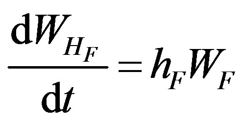
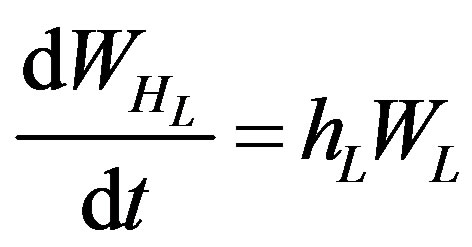
The dynamic model used was proposed by [19], and this was developed to indeterminate growth habit tomato under greenhouse conditions. This model starts from the flowering stage of the crop and has six state variables: mass balance for assimilation buffer (B), fruit dry weight (WF), leaf dry weight (WL), development stage (Dp), dry weight of harvested fruits (WHF) and dry weight of harvested leaves (WHL). The corresponding equations are described below:
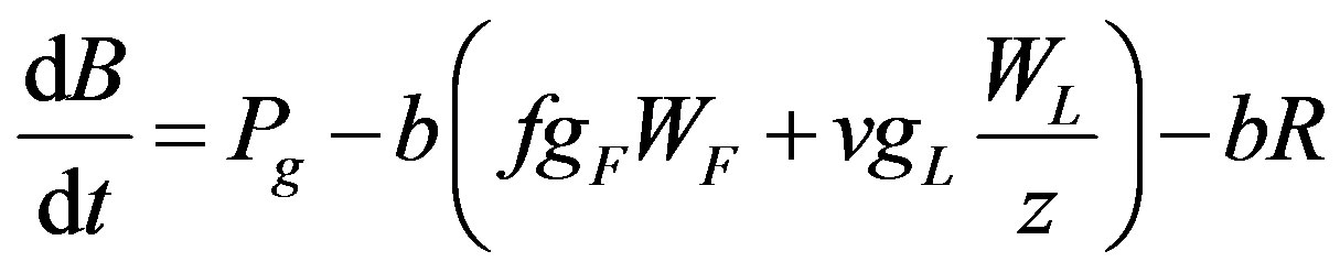 (1)
(1)
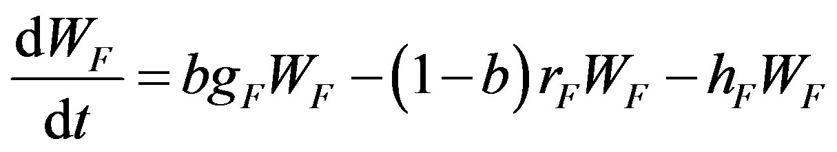 (2)
(2)
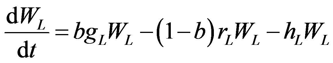 (3)
(3)
 (4)
(4)
 (5)
(5)
 (6)
(6)
Climate variables measured inside the greenhouse where used as input variables to the model (temperature, photosynthetically active radiation (PAR) and CO2). The outputs of the model are leaf dry weight (g·m−2), dry weight of fruit (g·m−2), harvested leaf dry weight (g·m−2) and harvested fruit dry weight (g·m−2). The complete description of the model is presented in [19] (Figure 1).
2.3. Calibration and Validation of the Tomato Growth Model
Model calibration was achieved by modifying the nominal values of a subset of parameters. These parameters, resulting from a sensitivity analysis, significantly affect model performance. The way this adjustment takes place is by modifying the nominal values of the model parameters and run the simulation model taking the input variables measured inside the greenhouse in the first growing season to find the values that give the best fit between simulated vs. observed outputs. Parameters were selected according to the sensitivity analysis performed by [19] plus some others that influence tomato varieties. Different values of these parameteres were tested until they met those providing more appropriate results when comparing the outputs of the model with real data of the first growing season (2011) of tomato.
To validate the model, climate data were taken from the second crop cycle as model inputs. The outputs of the same were compared with the actual data obtained from the second cycle (2012). To study the efficiency of the simulation of both the calibration and validation procedures, the “EF” and “Index” indexes given by [20] were used. These indices get values from 0 to 1, being 1 a perfect efficiency.
2.4. Modeling Mineral Content in Tomato
Nutrient demand mainly depends on the growth of the different plant organs, so that the maximum requirements are those when the plant has no limitation on the availability of these nutrients [21]. To generate behavioral models of the various minerals evaluated in the tomato plant, a simple regression technique is used. Time from flowering as well as actual mineral content in different organs of the plant for the first growing season (2011), were used. Six regression models corresponding to the six minerals (N, P, K, Ca, Mg and S) of higher concentration in each organ of the tomato plant were generated. The whole process of generating models was processed in Regress© (v. 2.21) for Excel.
The models generated were incorporated into the growth dynamic model to dynamically simulate the behavior of tomato minerals, because nutrients simulated concentration is equal to the plant demand if there is no limitation in the availability of nutrients [21]. This was done as follows:
 (7)
(7)
where OMC is the mineral content per organ (g·m−2) and ODW is the organ dried weight (g·m−2).
Since tomato growth model does not include dry
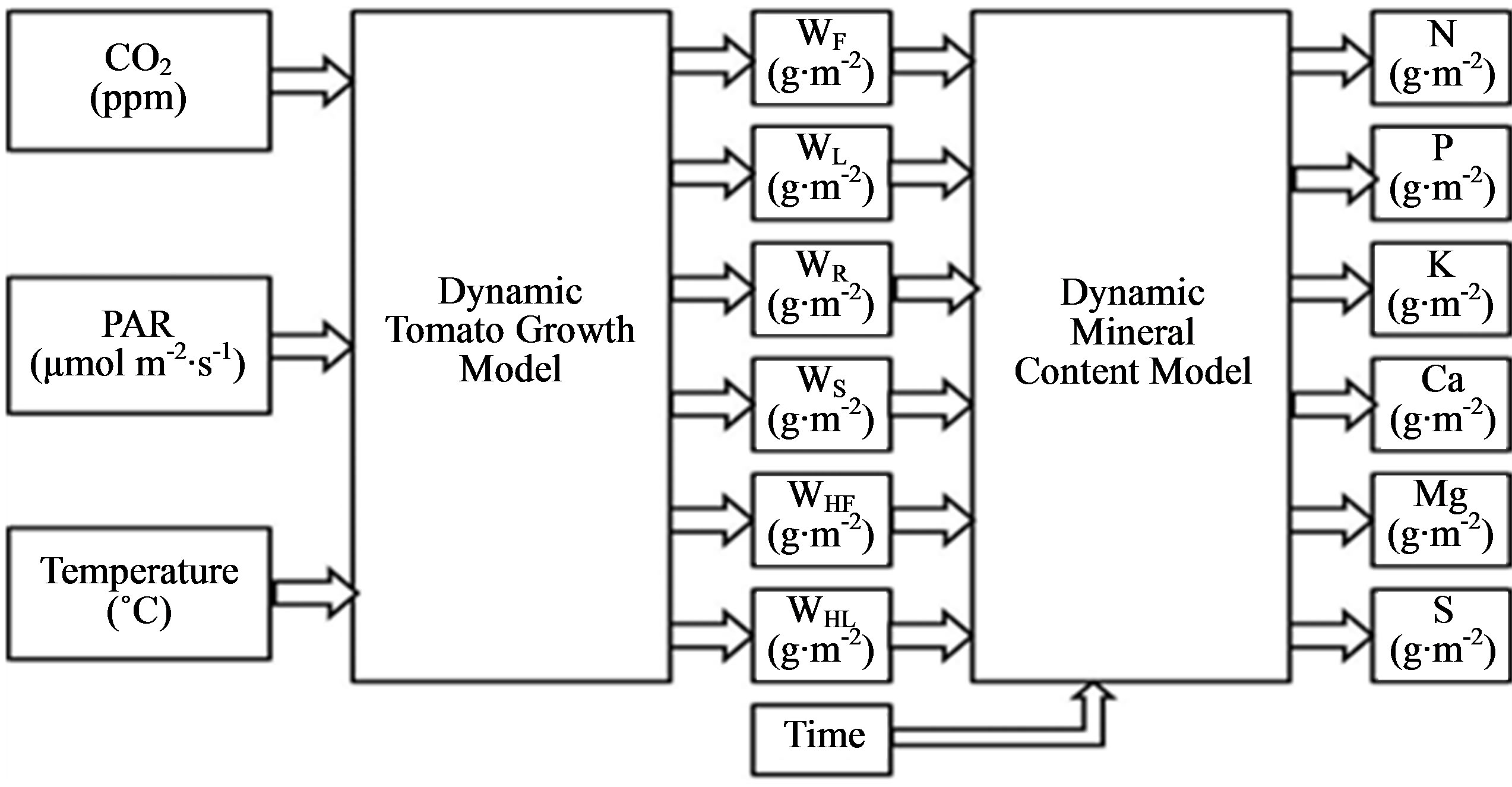
Figure 1. Block diagram of the tomato growth and mineral content models.
weights of stem and root as outputs, nor the total dry weight of leaves and fruits generated by the crop, the following equations were used:
 (8)
(8)
 (9)
(9)
where WS is the stem dry weight (g·m−2) and WR is the root dry weight (g·m−2). Both equations were obtained from linear regression.
 (10)
(10)
 (11)
(11)
where TWL is the total generated leaves dry weight (g·m−2) y TWF is the total generated fruit dry weight (g·m−2).
In order to assess the total mineral quantity for the plant, only mineral contents from the different organs were added.
 (12)
(12)
where TMC is the total mineral content (g·m−2), MCWS is the mineral content in the stem (g·m−2), MCWR is the mineral content in the root (g·m−2), MCTWL is the mineral content in the leaves (g·m−2), y MCTWF is the mineral content in the fruit (g·m−2).
TMC was considered only for the evaluation of the simulations of the six minerals (N, P, K, Ca, Mg and S) (Figure 1). Analogously to the modeling of growth of tomato plants, first crop cycle (2011) was used for the calibration of the mineral models used in the second cycle (2012). The whole programming process and dynamic simulation was performed in Matlab© R2011a.
3. RESULTS AND DISCUSSION
3.1. Modeling Growth of Tomato Plant
Following the calibration process, 11 parameters were modified out of a total of 27 available for the tomato growth model. Table 1 shows the evaluation for the different model outputs. It was observed that at 77 DAF only harvested leaves EF was less than 0.9 (0.8541), the rest was higher. In general at 84 and 91 DAF rates are lower than at 77 DAF, this is because growth was limited in the plants at 70 DAF, so real growth declined while the simulated one continued to grow (Figure 2). Table 2 shows the parameters of the model with their nominal values [19] and the values generated by the calibration process. Six of these parameters were slightly modified, and the rest (yL, mF, mL, f1 and d4) were greater in magnitude (Table 2). It is worth noticing that these parameters differ from those used by [19]. These differences are due to two main factors: the climate of the region where the experiments were carried out and the plant material used, since, each newly generated hybrid generated its own peculiarities regarding its technical management and absorption of nutrients [8].
Figure 2 shows the comparison of the actual data of the growing cycle of 2011 with the simulation result data obtained from the calibration. It is noted that the adjustment of the experimental observations concerning simulation is very good, because, in conducting the assessment with the indices “EF” and “Index” both showed a value greater than 0.95. Furthermore, WHL output gets values above zero from the start of the simulation (tomato flowering) unlike [19], which began tomato leaf pruning at the same time as tomato fruit harvesting (Figure 2). These differences are due to the use of different tomato hybrids, since as mentioned, each material has its own characteristics [8].
For the validation process of tomato growth model, unlike the work of [19], indices to assess the quality of the simulation model were used. In Table 3, the results of that assessment is shown. It was observed that the two indices used (EF and Index) are greater than 0.94 in the assessments made at 77 and 84 days after flowering (DAF) for WF, WL y WHF outputs.
Figure 3 shows the graphical comparison between the four outputs of the model and data from the tomato crop cycle 2012. It can be noticed the high quality of simulation at 84 DAF for WF, WL and WHF values. The output variable WHL, was underestimated by the model, this was because the management of pruning in the second growing season changed due to certain stress factors, forcing
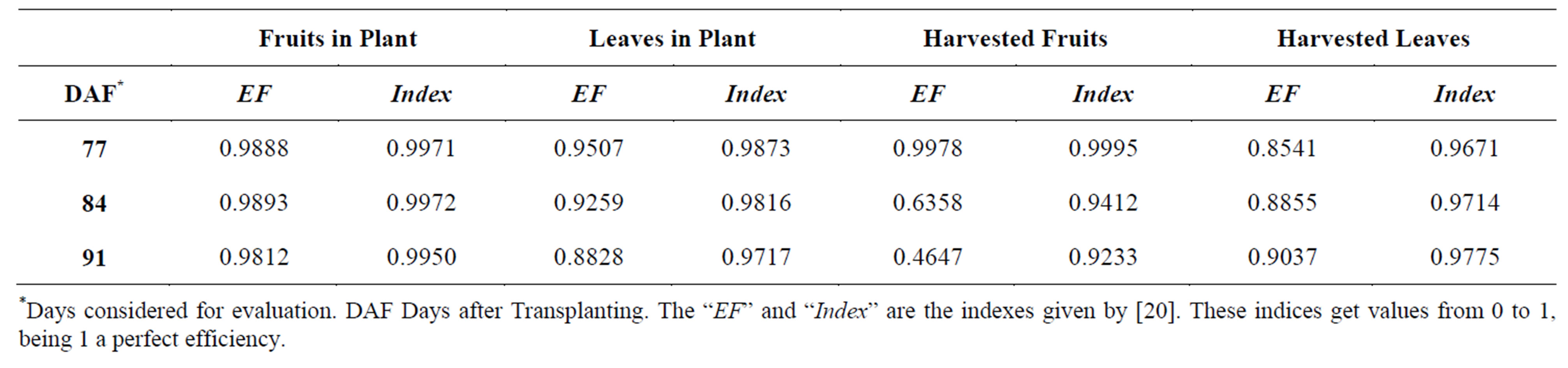
Table 1. List of indices used to evaluate the efficiency of the dynamic model simulation for different outlets in the calibration process.
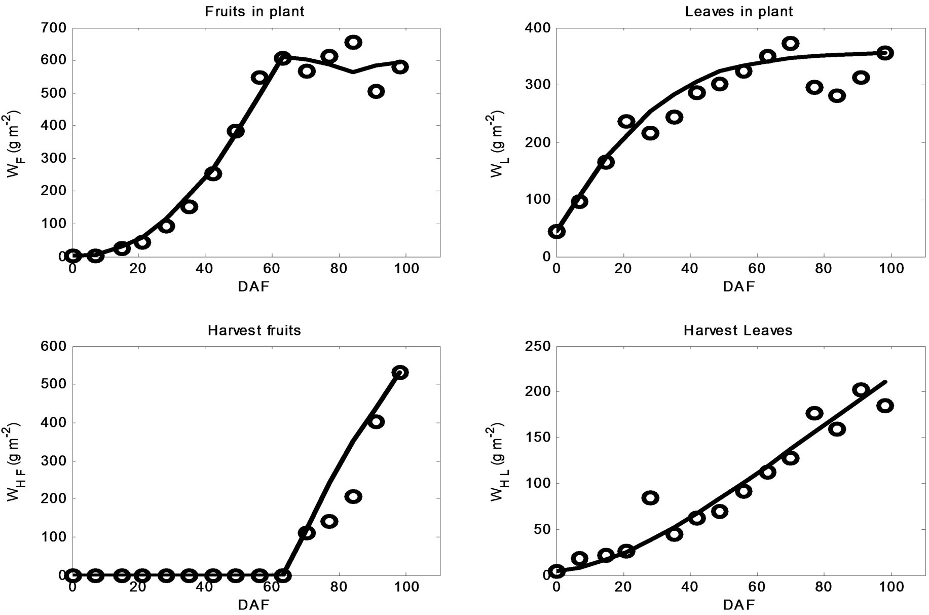
Figure 2. Calibration plots of model outputs. Real (o) vs. simulated (-) data comparison corresponding to cycle 2011.
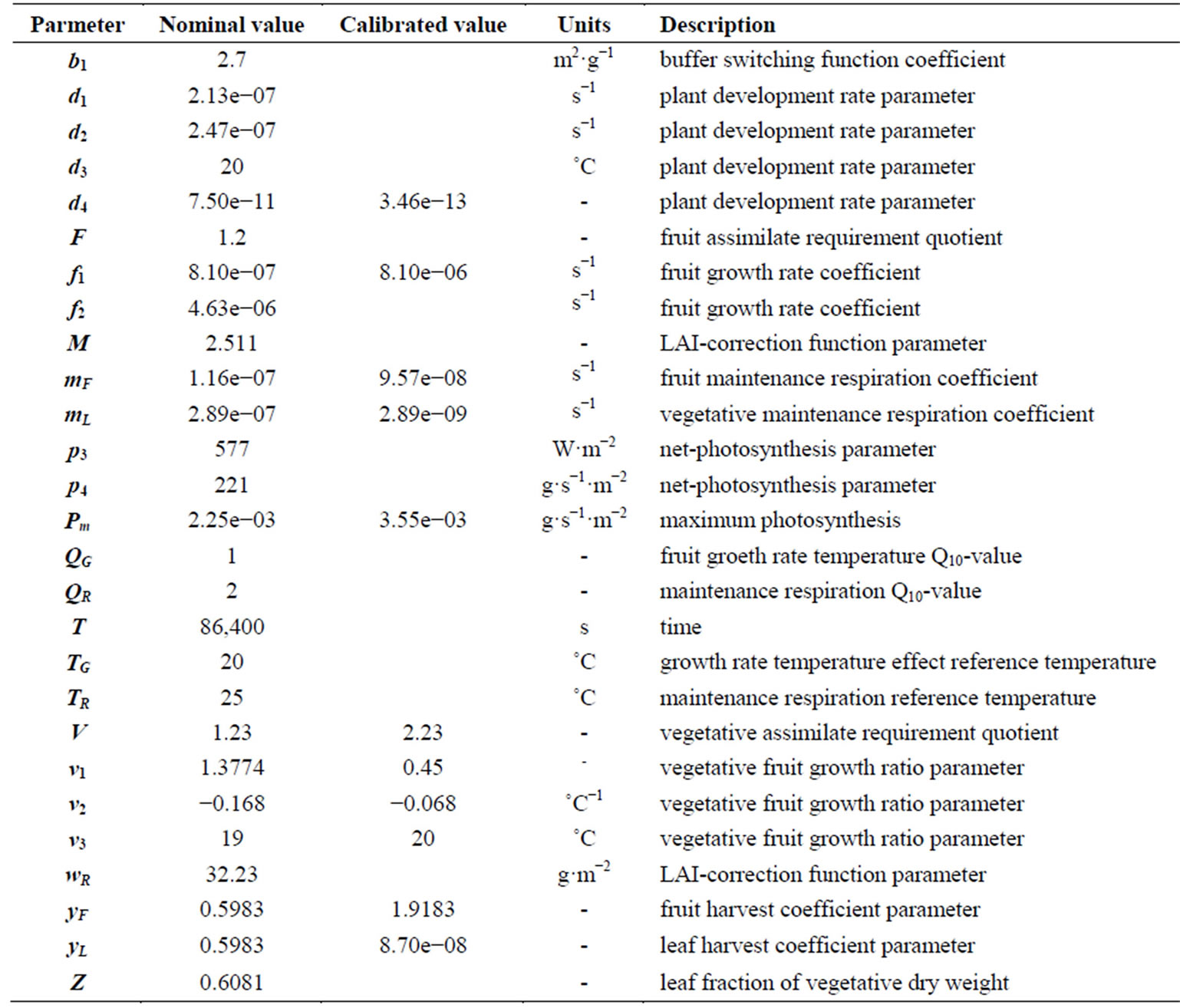
Table 2. Parameter description, nominal values [19] and calibrated values.

Table 3. Indices used to evaluate the efficiency of the dynamic model simulation for different outputs in the validation process. *Days considered for evaluation.
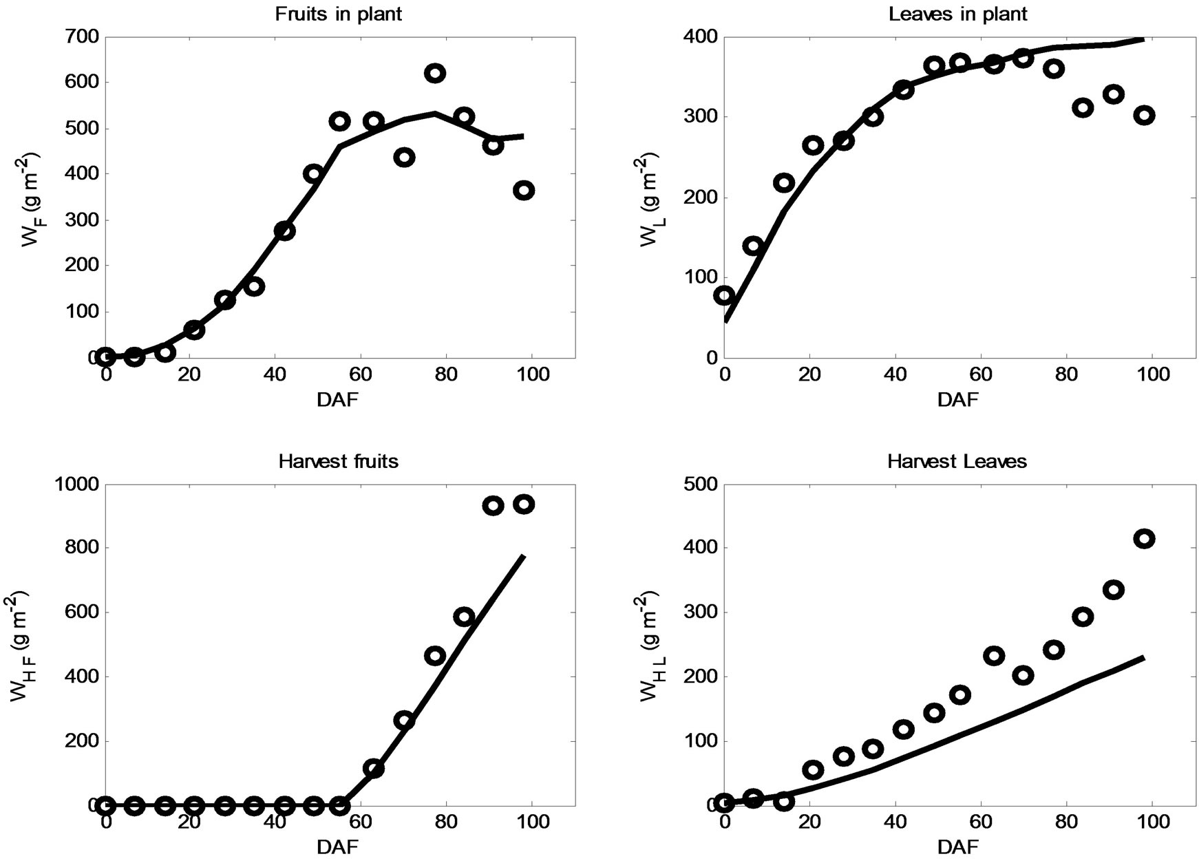
Figure 3. Model output plots. Cycle 2012 Real Data (o) vs. simulated output (-) are compared.
some extra mowing.
When evaluated at 91 DAF, best results were obtained for WHF (EF = 0.9676, Index = 0.9912) and WF (EF = 0.9679, Index = 0.9906). On the other hand, EF < 0.90 was obtained for both WL and WHL outputs (Table 3). These results should be explained as a result of the limited growth of tomato plants to 70 DAF, because in this case, the number of leaves on the plant as well as the number of leaves taken from the plant has decreased since then (Figure 3). Since the model is designed for indeterminate growth habit tomato, the simulation obtained by the same continues to grow while the actual values obtained from culture decrease (Figures 2 and 3). In the case of fruits, this is not the case, because by the time when growth was limited, there were still small fruits and flowers, so they continued to grow over time and harvesting continued (Figures 2 and3).
3.2. Mineral Modeling in Tomato Plants
The necessary models to mimic the behavior over time of minerals in tomato plants were generated from regression techniques. Table 4 shows the 24 regression models generated for the six minerals with higher concentration (N, P, K, Ca, Mg, S) and for the four tomato plant organs (leaf, stem, fruit and root). It was noted that 11 of the generated models are linear, 10 are quadratic, 2 are cubic, and just one of fourth order (Table 4). These results agree with [21], since the mineral concentration showed ontogenetic changes. In the particular case of the fruit, only nitrogen showed changes over time, and the remaining minerals (P, K, Ca, Mg and S) remained virtually unchanged (Table 4).
After entering the regression models generated for minerals in the dynamic model of tomato growth, a comparison between the simulated data and actual data of the growing season for 2011 was performed. Efficiency results of simulation are shown in Table 5. It is observed that for all minerals both indexes were higher than 0.95, a normally considered good efficiency. Although [21] performed nutrient modeling on peppers,
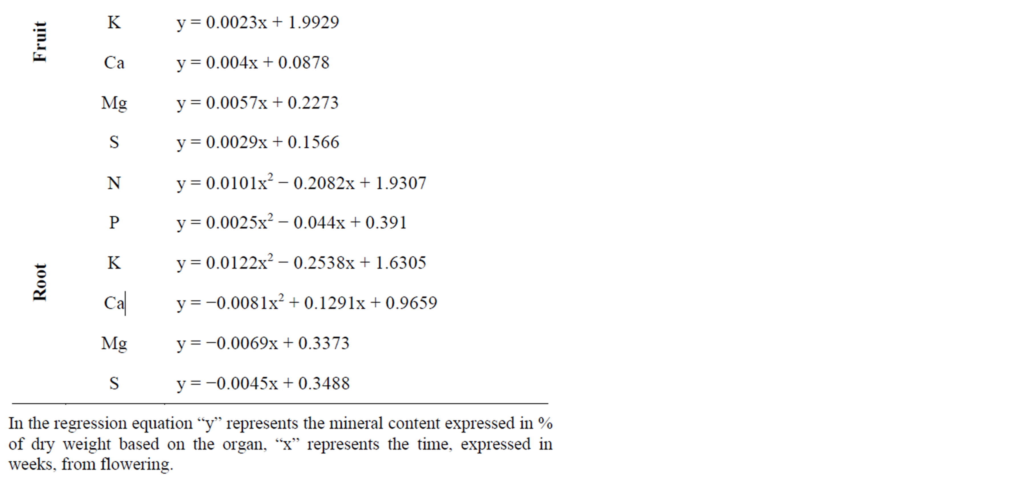

Table 4. Regression equations used to estimate minerals content in tomato plant.
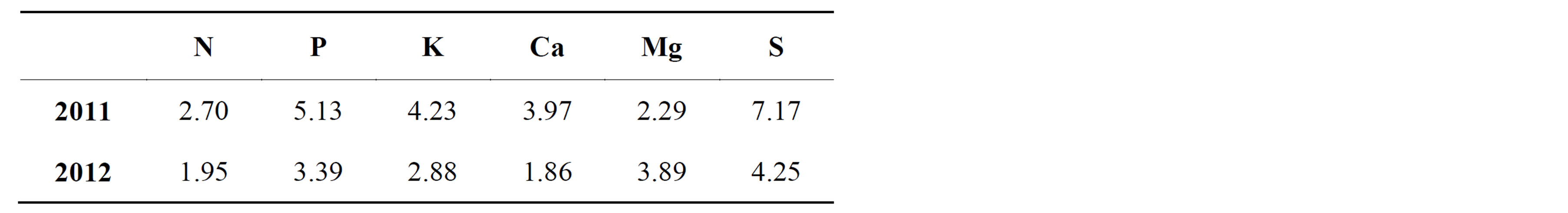
Table 5. Number of times minerals were applied during cultivation cycles.
there is no index to evaluate the efficiency of the model simulation.
Additionally, data corresponding to minerals applied to the crop by Steiner solution were included (Figure 4). It can be seen in the graphs presented in Figure 4 the good fit between the model simulated data and actual data of the six minerals in question.
To validate the modeling of minerals (N, P, K, Ca, Mg and S) in tomato plants, simulated values were compared against those obtained from the crop cycle conducted in 2012 (Figure 5). Efficiency results of simulation are shown in Table 5. In this case it was found that the simulations corresponding to N, P, K and S showed very good fit because both indices used were higher than 0.95. This is borne out graphically in Figure 5. Regarding Ca and Mg, EF values of 0.75 and 0.89, respectively, were obtained. Model underestimated the Ca content as measured value was higher in plants by approximately 61% at 98 days after transplantation (DAT). On the other hand, the Mg content was overestimated by the model by 62% in the same time period (Figure 5). These results can be explained due to errors in the simulation of growth and its partitioning into the different plant organs [21], since as shown in Table 3, simulation efficiency for harvested leaves was very low (EF = 0.64).
Although mineral simulation in tomato has already been reported, this was based on variations in the concentration of minerals in the nutrient solution or drain using a mass balance equation based on the concept of concentration ion extraction [17]. In contrast, in this paper, actual mineral concentrations in the different organs of the tomato plant are considered.
Considering the presented results, some adjustments can be made based to the management of fertilization of greenhouse tomato plants by means of daily quantification of nutrient demand [9]. This helps us prevent shortfalls or excesses of nutrients in the tomato plants, which in turn will reduce production costs without affecting production either in quantity or in quality. In addition, by allowing the simulation of minerals to be based on tomato growth, which in turn depends on the climate in which it operates, we can design management practices that increase productivity while minimizing environmental impact caused by the agriculture activity [10].
Regarding the actual application of minerals to tomato plants during the time the cultures were grown, Figures 4 and 5 show the comparison of these data with the simulated and measured data in the culture. Additionally, Table 5 shows the relationship between the amount of minerals applied and measured in tomato plants during both cycles of cultivation. It can be noticed that S is most excessively applied mineral in both tomato crop cycles, namely 7.17 times in 2011 and 4.25 times in 2012. P was the second most applied mineral with 5.13 times in 2011 and 3.39 times in 2012. The N and Ca were those applied in smaller excess in the 2012 cycle, with 1.95 and 1.86 times respectively. It should be considered that while the S is essential for the growth and development of plants, it has been documented that higher applications of S, lower
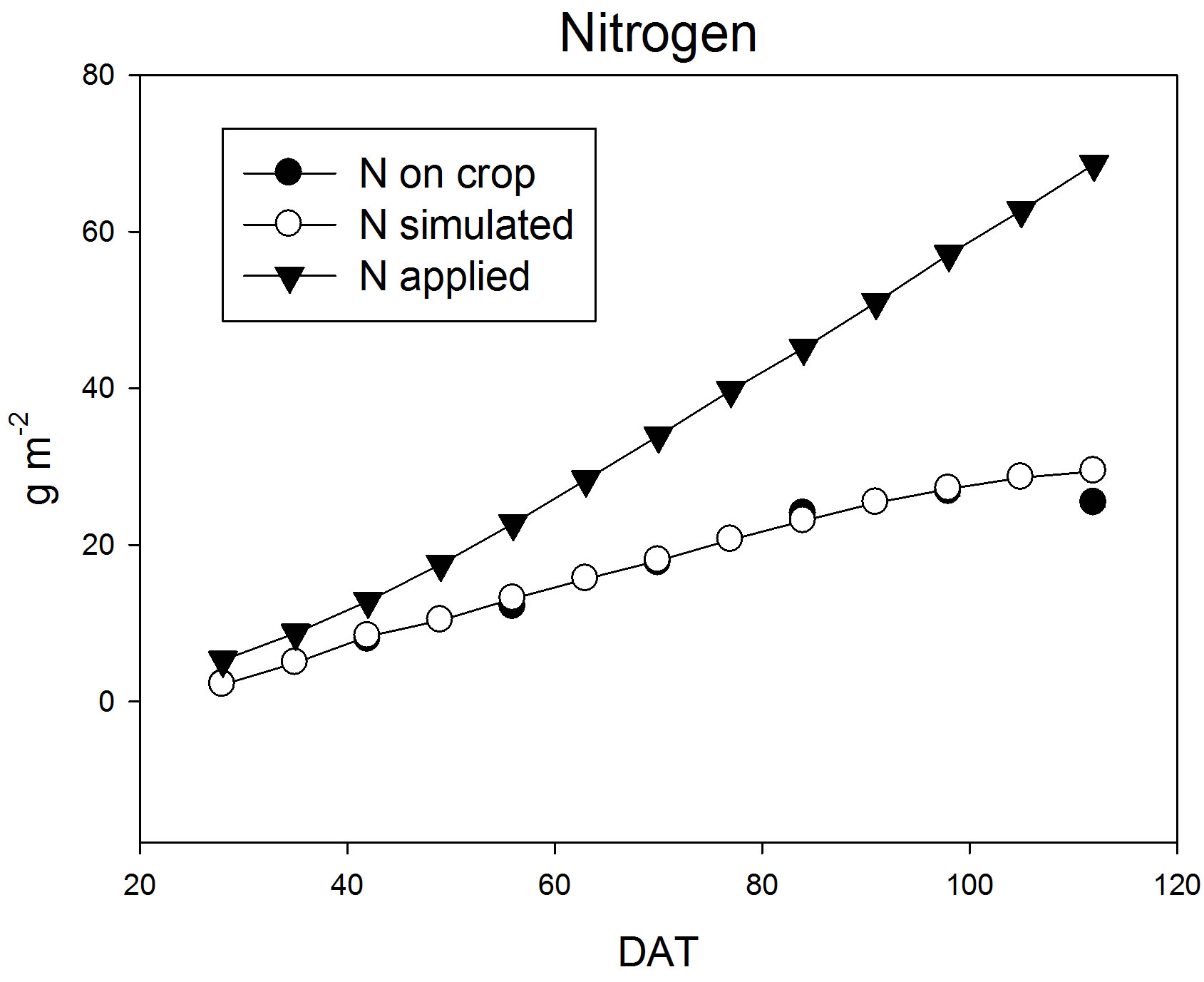
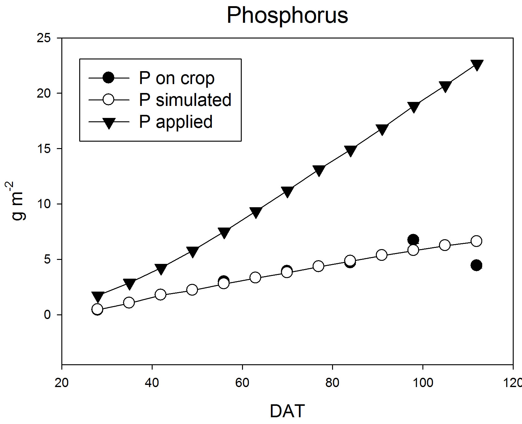
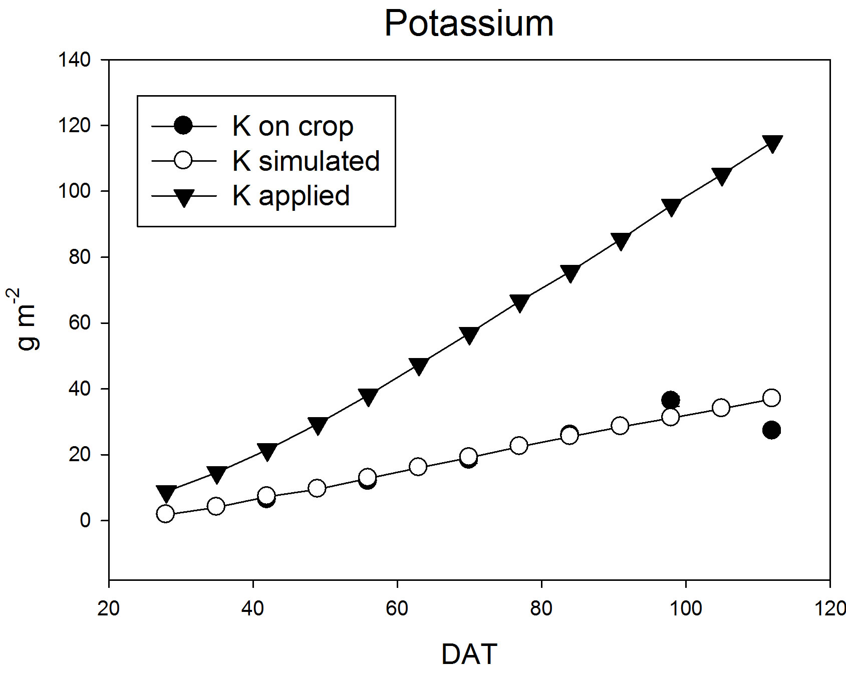
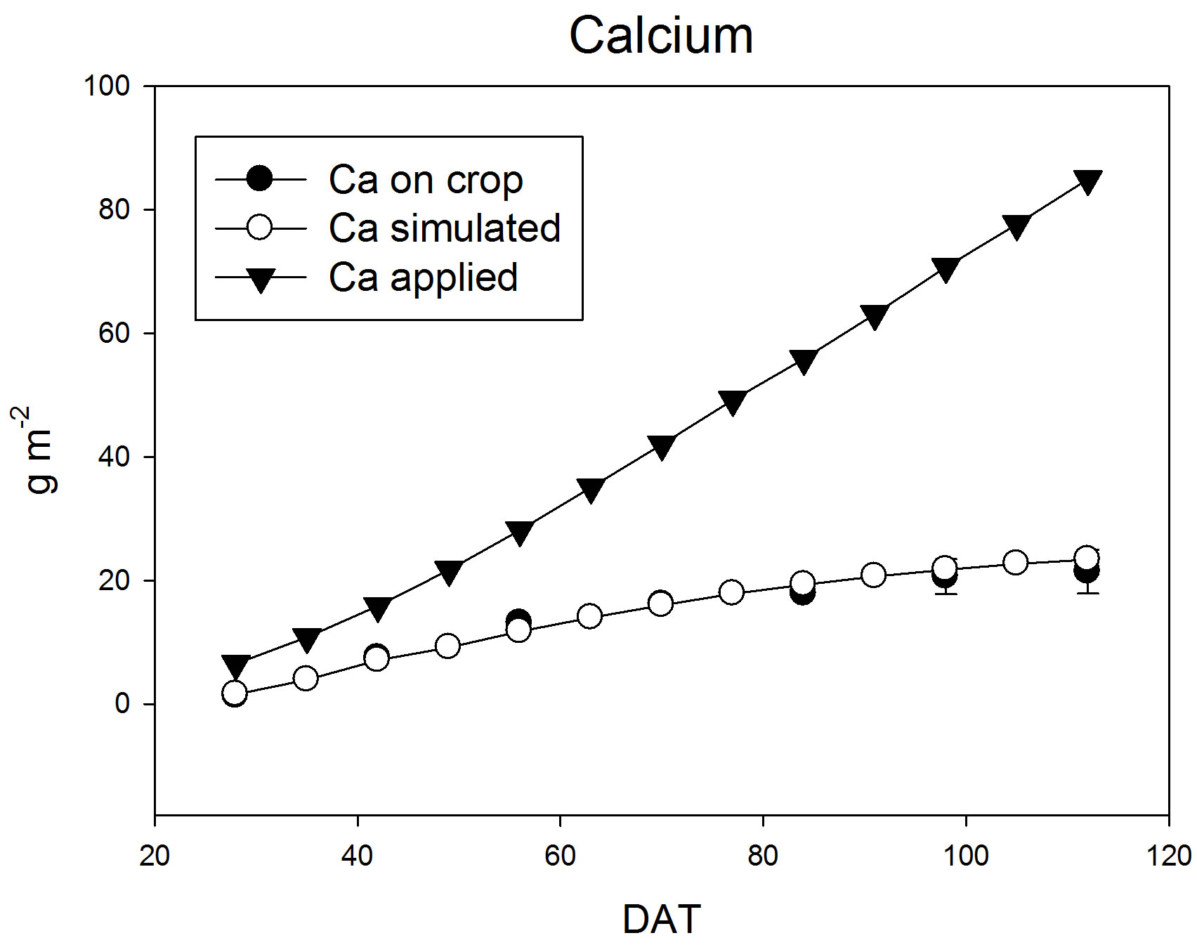
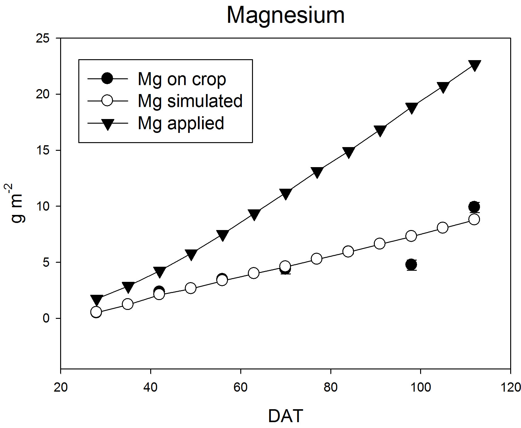
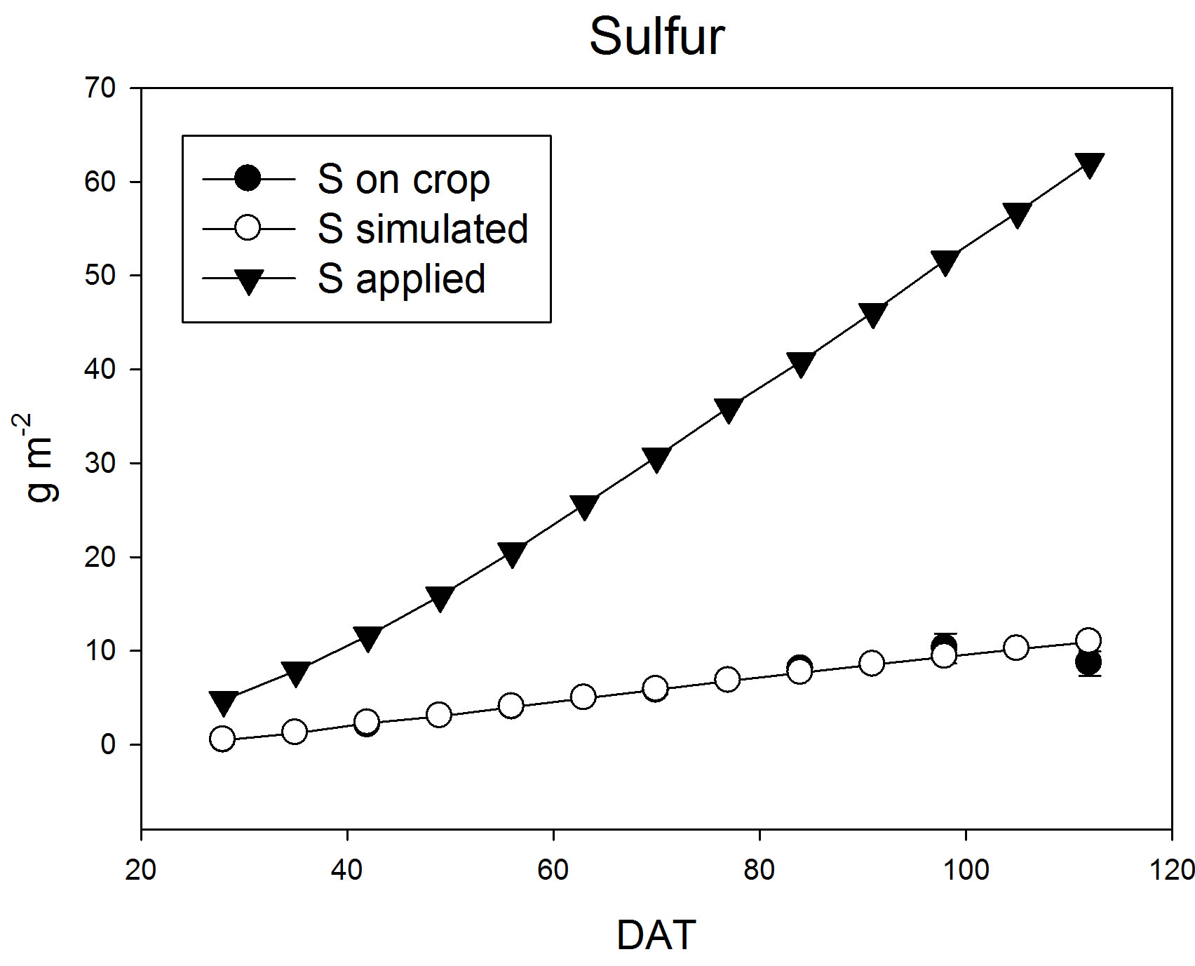
Figure 4. Calibration plots showing mineral content in tomato plant. Real quantity of minerals applied using Steiner solution is included.
Cu concentration in the tomato plant, and soil salinity increases [22].
These results show that we must consider several important issues for the production: the increase in the cost of mineral fertilizers and their availability in the future [4,5,11] as well as the impact on the environment on overuse of fertilizers [3,11]. In this sense, the modeling techniques proposed in this work can support in managing the nutrition of tomato plants. Extraction curves allow nutrient demand according to the phenological stage of the crop, so that can be used to establish fertilization programs in order to maximize its efficiency [8]. This is consistent with [12], since the use of these models has a significant impact on the economic and ecological benefits.
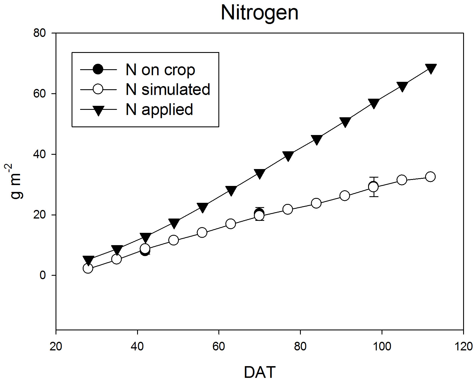
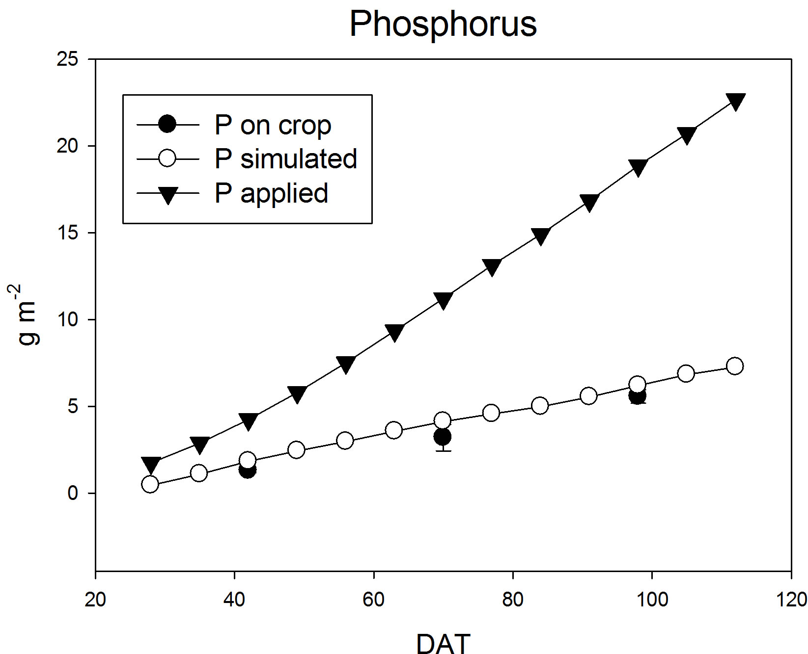
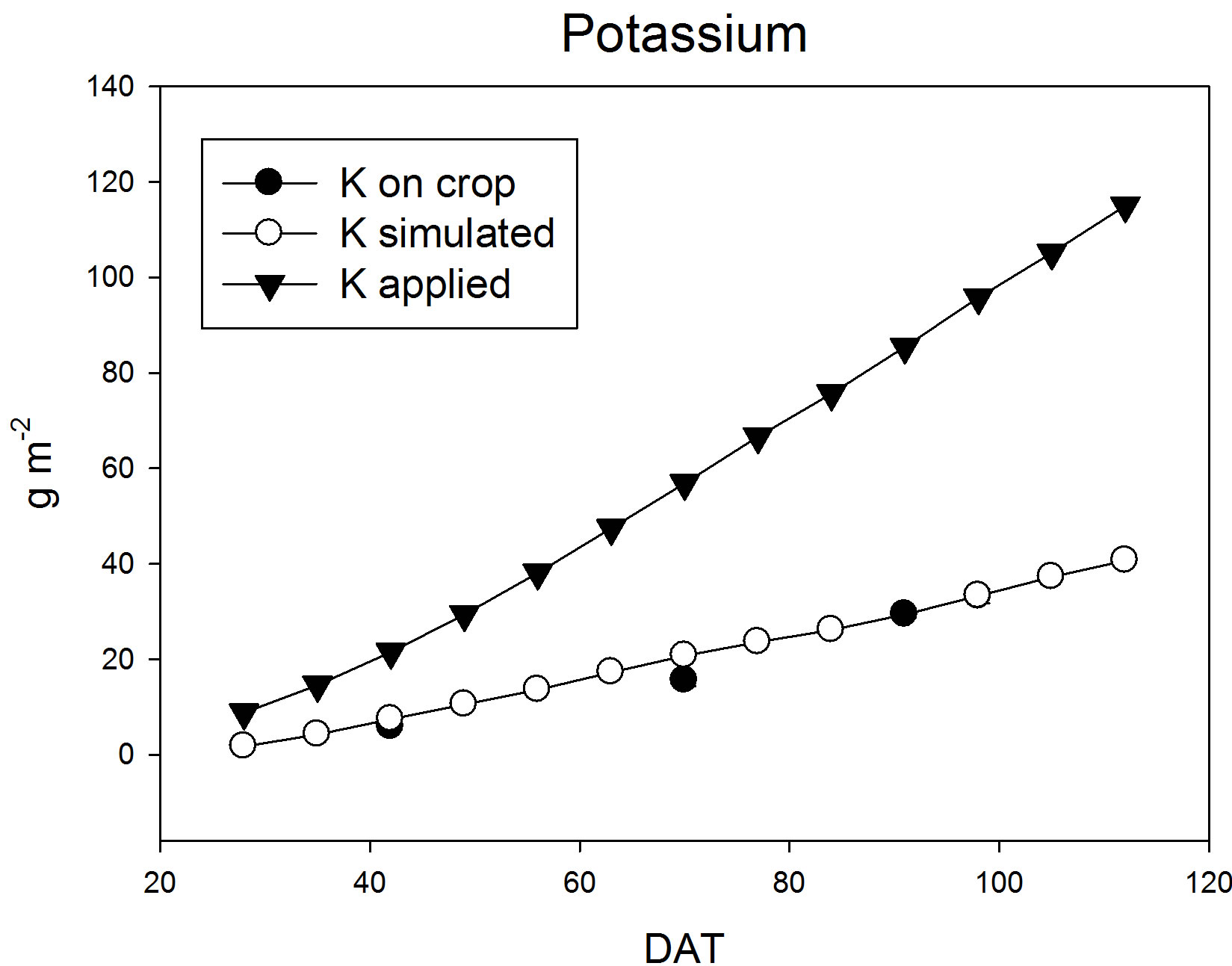

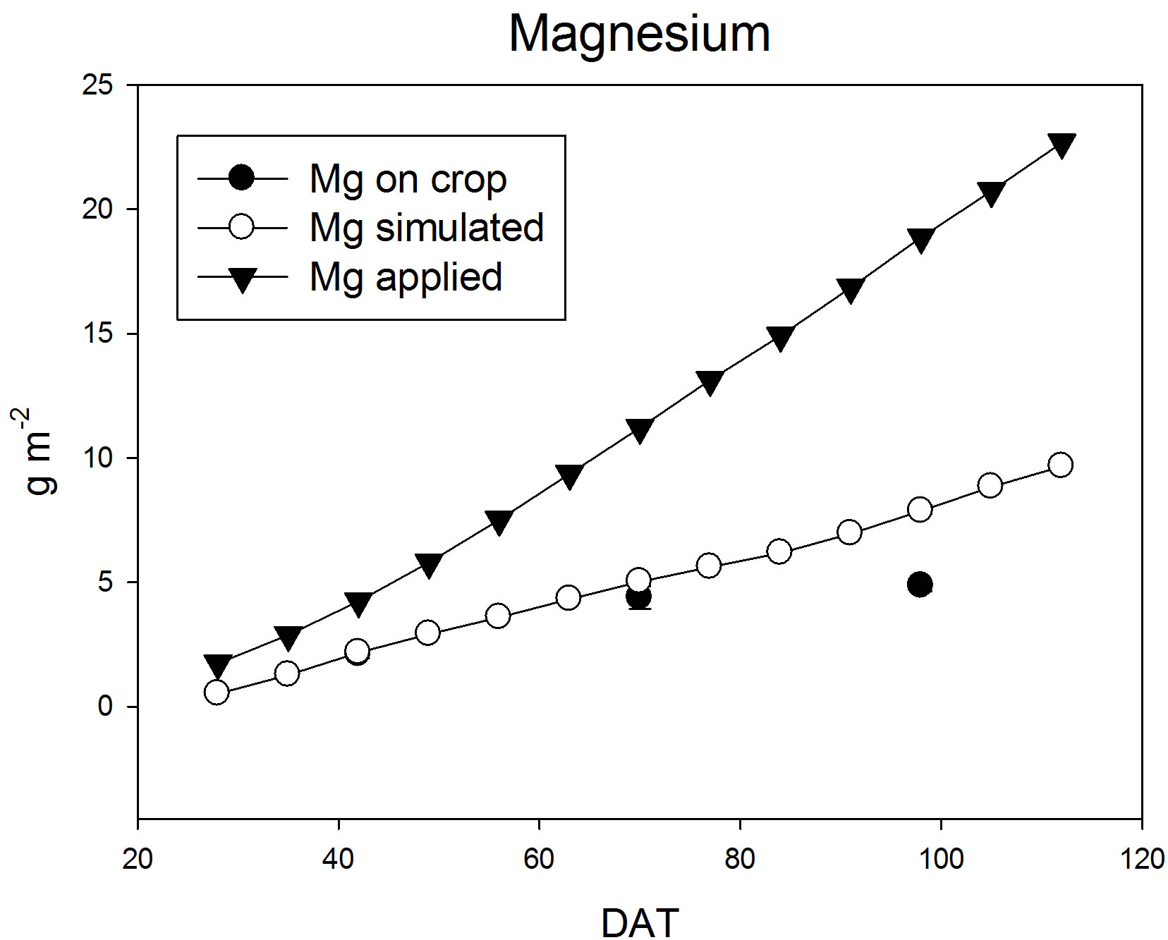
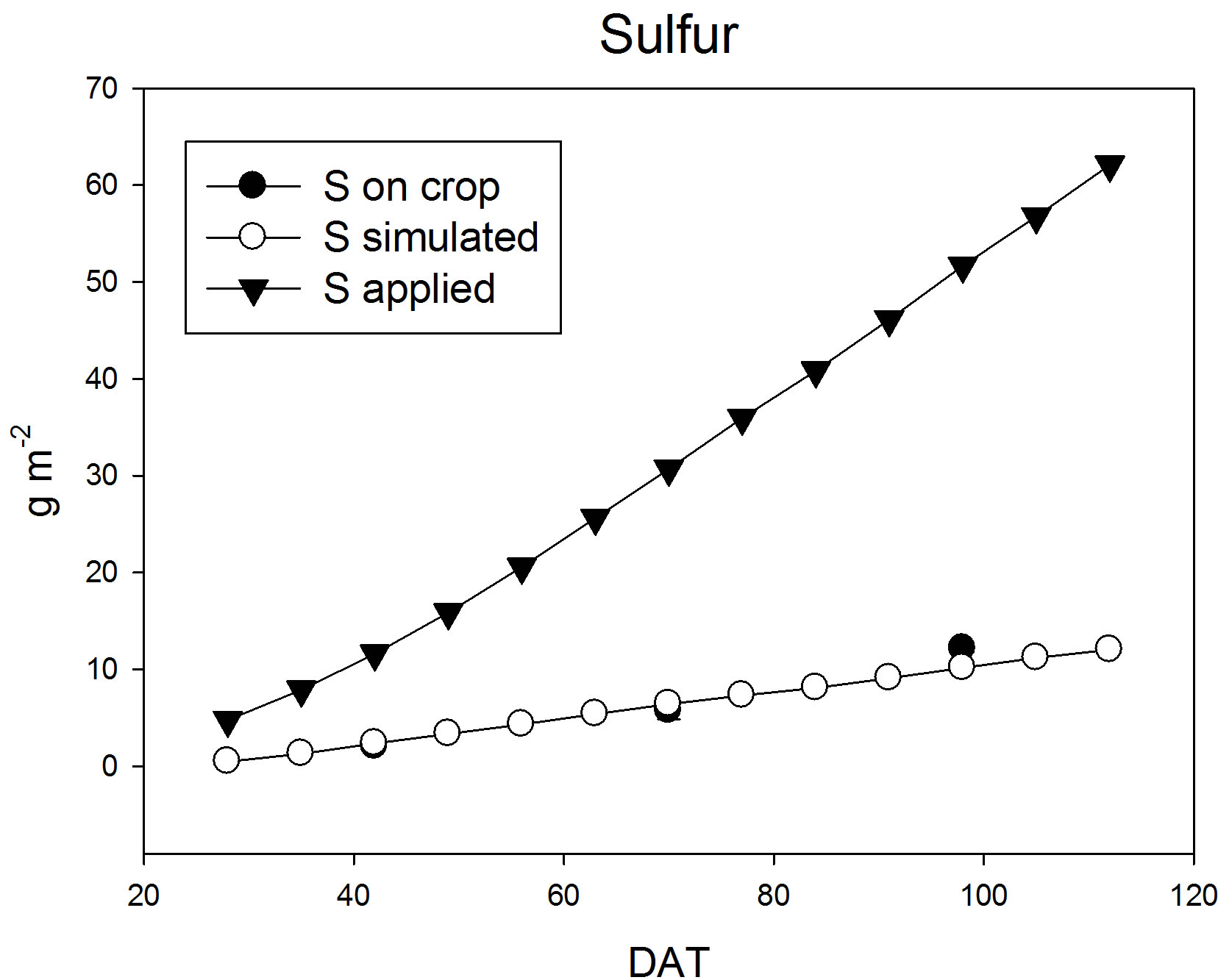
Figure 5. Validation plots showing mineral content in tomato plant. Real quantity of minerals applied using Steiner solution is included.
4. CONCLUSSIONS
In this work, it was calibrated and validated a dynamic model of tomato growth under greenhouse conditions which can be used to design appropriate strategies for the management of this crop.
Several regression models generated from measurements of the concentrations of N, P, K, Ca, Mg and S in the various organs of the tomato plants and they were incorporated into the dynamic model of tomato growth. This model allows us to simulate the nutritional requirements for tomato plants under greenhouse conditions from weather conditions existing within it. This model can be used as support for the management of mineral fertilization of tomato.
The application of these modeling and simulation techniques can minimize the use of fertilizers for greenhouse tomato crop, allowing us to estimate very precisely the nutritional requirements. This will generate, as a result, a decrease in production costs and reduce environmental impact by excessive application of fertilizers in the cultivation of tomato, all without affecting the production and quality.
REFERENCES
- Martínez-Ruiz, A., López-Cruz, I.L., Ruiz-García, A. and Ramírez-Arias, A. (2012) Calibración y validación de un modelo de transpiración para gestión de riegos de jitomate (Solanum lycopersicum L.) en invernadero. Revista Mexicana de Ciencias Agrícolas, 4, 757-766.
- SAGARPA (2013) Agricultura protegida 2012. http://www.sagarpa.gob.mx/agricultura/Paginas/Agricultura-Protegida2012.aspx
- Sepat, N.K., Kumar, A., Yadav, J. and Srivastava, R.B. (2012) Effect of integrated nutrient management on growth, yield and quality of tomato in trans Himalayan. Annals of Plant and Soil Research, 14, 120-123.
- Gad, N. and Hassan, N.M.K. (2013) Role of cobalt and organic fertilizers amendments on tomato production in the newly reclaimed soil. World Applied Sciences Journal, 22, 1527-1533.
- Mehdizadeh, M., Darbandi, E.I., Naseri-Rad, H. and Tobeh, H. (2013) Growth and yield of tomato (Lycopersicon esculentum Mill.) as influenced by different organic fertilizers. International Journal of Agronomy and Plant Production, 4, 734-738.
- Shalaby, T.A. and El-Banna, A. (2013) Molecular and horticultural characteristics of in vitro induced tomato mutants. Journal of Agricultural Science, 5, 155-163.
- MÉXICOPRODUCE (2013) Productos: Jitomate. http://www.mexicoproduce.mx/productos.html#jitomate
- Quesada-Roldán, G. and Bertsh-Hernández, F. (2013) Obtaining of the absorption curve for the fb-17 tomato hybrid. Terra Latinoamericana, 31, 1-7.
- Bugarín-Montoya, R., Galvis-Spinola, A., Sánchez-García, P. and García-Paredes, D. (2002) Daily accumulation of aboveground dry matter and potassium in tomato. Terra Latinoamericana, 20, 401-409.
- Enriquez-Reyes, S.A., Alcántar-González, G., CastellanosRamos, J.Z., Suárez, E.A., González-Eguiarte, D. and Lazcano-Ferrat I. (2003) NUMAC-N Tomato: Mineral nutrition fit at growth. The nitrogen nutrition in tomato greenhouse production. 1. Model description and parameters adjust. Terra Latinoamericana, 21, 167-175.
- Basheer, M. and Agrawal, O.P. (2013) Effect of vermicompost on the growth and productivity of tomato plant (Solanum lycopersicum) under field conditions. International Journal of Recent Scientific Research, 4, 247-249.
- Zhang, J. and Wang, S. (2011) Simulation of the canopy photosynthesis model of greenhouse tomato. Procedia Engineering, 16, 632-639. http://dx.doi.org/10.1016/j.proeng.2011.08.1134
- Marcelis, L.F.M., Elings, A., Bakker, M.J., Brajeul, E., Dieleman, J.A., de Visser, P.H.B. and Heuvelink, E. (2006) Modelling dry matter production and partitioning in sweet pepper. Acta Horticulturae, 718, 121-128.
- Gary, C. (1999) Modeling greenhouse crops: State of the art and perspectives. Acta Horticulturae, 495, 317-322.
- De Gelder, A., Heuvelink, E. and Opdam, J.J.G. (2005) Tomato yield in a closed greenhouse and comparison with simulated yields in closed and conventional greenhouses. Acta Horticulturae, 691, 549-552.
- Marcelis, L.F.M., Elings, A., de Visser, P.H.B. and Heuvelink, E. (2009) Simulating growth and development of tomato crop. Acta Horticulturae, 821, 101-110.
- Massa, D., Incrocci, L., Maggini, R., Bibbiani, C., Carmassi, G., Malorgio, F. and Pardossi, A. (2011) Simulation of crop water and mineral relations in greenhouse soilless culture. Environmental Modelling and Software, 26, 711-722. http://dx.doi.org/10.1016/j.envsoft.2011.01.004
- Steiner, A.A. (1961) A universal method for preparing nutrient solutions of a certain desired composition. Plant Soil, 15, 134-154. http://dx.doi.org/10.1007/BF01347224
- Tap, R.F. (2000) Economics-based optimal control of greenhouse tomato crop production. Ph.D. Dissertation, Wageningen Agricultural University, Wageningen.
- Wallach, D. (2006) Evaluating crop models. In: Wallach, D., Makowski, D. and Jones, J.W., Eds., Working with Dynamic Crop Models. Evaluation, Analysis, Parameterization and Applications, Elsevier, Amsterdam, 11-54.
- Marcelis, L.F.M., Brajeul, E., Elings, A., Garate, A. and Heuvelink, E. (2005) Modelling nutrient uptake of sweet pepper. Acta Horticulturae, 691, 285-292.
- Orman, S. (2012) Effects of elemental sulphur and farmyard manure applications to calcareous saline clay loam soil on growth and some nutrient concentrations of tomato plants. Journal of Food, Agriculture & Environment, 10, 720-725.