American Journal of Plant Sciences
Vol.5 No.6(2014), Article ID:44098,13 pages DOI:10.4236/ajps.2014.56096
Maize Cultivar Specific Parameters for Decision Support System for Agrotechnology Transfer (DSSAT) Application in Tanzania
Sixbert Kajumula Mourice1*, Cornell Lawrence Rweyemamu1, Siza Donald Tumbo2, Nyambilila Amuri3
1Department of Crop Science and Production, Sokoine University of Agriculture, Morogoro, Tanzania
2Department of Agricultural Engineering and Land Planning, Sokoine University of Agriculture, Morogoro, Tanzania
3Department of Soil Science, Sokoine University of Agriculture, Morogoro, Tanzania
Email: *sixbert.mourice@gmail.com
Copyright © 2014 by authors and Scientific Research Publishing Inc.
This work is licensed under the Creative Commons Attribution International License (CC BY).
http://creativecommons.org/licenses/by/4.0/


Received 7 January 2014; revised 13 February 2014; accepted 1 March 2014
ABSTRACT
In order to develop basis for tactical or strategic decision making towards agricultural productivity improvement in Tanzania, a new approach in which crop models could be used is required. Crop specific parameters for maize cultivars in Tanzania have not been determined before and consequently; crop modeling approaches to address biophysical resource management challenges has not been effective. The objective of this study was to evaluate DSSAT (v4.5) Cropping System Model (CSM) using four adapted maize cultivars namely Stuka, Staha, TMV1 and Pioneer HB3253 for quantifying model parameters. The results indicate that maize cultivars did not differ significantly in terms of the number of days to anthesis, maturity, or grain weight except final aboveground biomass. Also, there was no difference between variables with respect to growing seasons. The cultivar specific parameters obtained were within the acceptable range of those for a hypothetical maize medium season cultivar (990002) included in the DSSAT 45 CSM. Model evaluation results indicate that using the estimated cultivar coefficients, the model simulated well the effects of varying nitrogen management as indicated by the agreement index (d-statistic) closer to unity. Therefore, it is concluded that model calibration and evaluation was satisfactory within the limits of test conditions, and that the model fitted with cultivar specific parameters can be used in simulation studies for research, farm management or decision making.
Keywords:CERES-Maize; Crop System Model; Nitrogen; Phenology; Morogoro

1. Introduction
Crop models have been developed and used worldwide as operational or strategic research and decision support tools in crop production or resources management. For example, in the Netherlands, average farmer’s wheat yield was below 5 t/ha in 1960’s while crop had predicted a potential yield of 10 tons/ha. By 1993, the yields had exceeded 9 tons/ha [1] . Crop models are also being used to evaluate the impact of climate change on crop production as a result of increased green-house gases ([2] [3] ). In resource management optimization, crop models have played an important role, for example, Agricultural Productivity Simulator (APSIM) model has been used to develop an understanding of long-term effects of conservation agriculture on the productivity of smallholder systems in Zimbabwe [4] .
Tanzania has had several initiatives geared towards agricultural intensification country-wide, dating back to independence times (e.g. “siasa ni kilimo”, (of 1972), “kilimo cha kufa na kupona” (of 1974/75) and recent “Kilimo Kwanza” (of 2010)), which have had little or no impact on as far what agricultural productivity improvement is concerned. For instance, maize which is the most important staple grain, grown on 44% of total cultivated area and accounting for 62% of total cereal production [5] has seen its yields declining [6] , despite the fact that area under maize cultivation has on average been increasing, at an average rate of 8 per cent per year for the past 20 years. Generally, maize yields are very low, averaging 1.2 tons/ha [5] , suggesting that maize production has not matched with population growth as evidenced by a surge in maize grain imports to address the deficit [6] .
To be able to develop basis for tactical or strategic decision making to improve agricultural productivity in Tanzania, a new approach in which crop models could be used is required. To date, there have been some efforts in evaluating or adapting some dynamic crop models in Tanzania. However, the progress has been slow. Since most models have been developed elsewhere in Europe and USA, their use outside their domain of development requires a great deal of data for their calibration and validation, which is not readily available or difficult to obtain. The most important aspects in evaluating crop models include determination of cultivar specific parameters or coefficients [7] . Cultivar coefficients for maize varieties in Tanzania are not known and are not included in the cultivar database of DSSAT version 4.5 [8] . As a result, it is difficult to understand underlying processes that impact on crop yield, and therefore it may be difficult in designing appropriate strategies to improve crop productivity as well as efficient resource use. Previous studies using crop models have succumbed to serious shortfalls due to lack of crop cultivar parameters and either opted for generic models or used surrogate maize cultivars, the result of which could lead to more uncertainty in the results.
Mwandosya et al. [9] projected that countrywide maize yield declines by 33%, and temperature rises between 2˚C - 4˚C by end of this century as a result of doubling atmospheric CO2 concentration. The setback encountered in their study was that there were no experimental data as regards to growth, development and yield for the maize cultivar (Ukiriguru Composite) used in CERES-Maize simulations. Thus, it was difficult to obtain the cultivars’ parameters for sufficient model calibration hence high chances for erroneous outputs. Lack of crop cultivars whose genetic parameters are known, has led Harvest Choice [10] to using generic maize cultivars predicting yield gaps under rain-fed conditions in Sub Saharan Africa. Moreover, generic models which need few crop data, for example CLICROP, have also been used in Tanzania for climate change studies [11] . Model predictions would have been greatly improved had there been sufficient information over crop cultivar coefficients.
Several approaches for estimating cultivar coefficients have been documented. However, these approaches require key information regarding a particular crop cultivar such as planting dates, anthesis and physiological maturity dates and final grain yield, which in most cases are not available. Anothai et al. [12] used genetic coefficient calculator (GENECALC) which is a sub module in the Decision Support System for Agrotechnology Transfer (DSSAT v4.5) to determine cultivar coefficients for new peanut lines in Thailand from standard varietal trials. Bannayan and Hoogenboom [13] employed pattern recognition technique, which is based on similarity measures to estimate crop cultivar coefficients for maize. He et al. [14] used generalized likelihood uncertainty estimation (GLUE) method to estimate maize cultivar coefficients. Also DSSAT v4.5 has GLUE module for estimating crop cultivar coefficients [8] . All of the aforementioned approaches to estimate crop cultivar coefficients for use in dynamic crop models need some degree of information on a particular cultivar. Therefore, in situations where there are paucity of data from standard variety trials or other dedicated experiments, repeated field experimentations would be the only option.
Accurate estimation of crop cultivar coefficients is the entry point into dynamic crop model use (for research as well as decision making) and improvement for identification and consequently narrowing gaps in our knowledge over crops and biophysical aspects for improved agricultural productivity. Calibrated crop models with cultivar parameters can be used to optimize crop management [15] ), to evaluate the impacts of climate change [16] , to develop options to optimize resource use [4] or to develop new crop genotypes [17] .
Since maize cultivar coefficients for use in DSSAT CSM have not been investigated under Tanzanian environment, an overall objective of this work was to quantify the maize cultivar coefficients for four maize cultivars adapted for the lowland and mid altitude agro ecologies. Specific objectives were 1) to determine maize crop growth and development indices under optimum conditions (2) to estimate maize cultivar parameters and calibrate DSSAT CSM using the same, and (3) to evaluate DSSAT CSM for simulating maize growth and yield under the Wami-Ruvu River Basin (WRB) conditions.
2. Materials and Methods
The study site is within Morogoro region, characterized by a bimodal rainfall pattern with short rains for some years between October and December and long rains from March to June. The site receives annual precipitation of 850 mm (of which 65% - 75% fall between March and June) and an average daily temperature of 24˚C. The soils of the study site were characterized as isohyperthermic, Ultic Haplustalfs, with good natural drainage, and a slope of between 1% - 2%.
2.1. CERES-Maize Model Description
CERES (Crop-Environment-Resource-Synthesis)—Maize module [18] within the DSSAT v (4.5) requires minimum data sets (MDS) [7] to compute daily growth of vegetative and reproductive components as a function of daily photosynthesis, growth stage, and water and nitrogen stresses. A detailed account on MDS and data for evaluation of DSSAT-family crop models have been documented elsewhere [7] [19] [20] . CERES-Maize requires a set of six cultivar specific parameter for its calibration (Table 1).
2.2. Field Experiments for Model Calibration
Two field experiments were carried out at Sokoine University of Agriculture within the crop museum site (6˚50′58ʺ S and 37˚39′56ʺ E, 540 m above sea level) during 2011/2012 and 2012/2013 growing seasons. The site was previously planted to upland rice. Four adapted maize cultivars, namely Pioneer Phb 3253, Situka, Staha and TMV1 were selected for use in this experiment following a key-informants interview in Morogoro, Kilosa, Kongwa Kiteto and Kilindi districts. The respondents included district and ward agricultural officers, farmers and agro-input stockists. Pioneer Phb 3253 is a full season hybrid cultivar with dented type of grain with yield potential ranging from 5 to 6.5 tons/ha. Situka is an open pollinated cultivar (OPV) yielding between 4.0 - 6.0 tons/ha. TMV1 is also an OPV with yield potential of 4.0 ton/ha while Staha yields between 4 - 5 tons/ha. Plant population for each cultivar was 44,000 plants/ha. The maize cultivars were planted in a completely randomized block design with three replications. Sowing was done on March, 07 for the 2011/2012 season and on similar date for the 2012/2013 season. In both growing seasons, each plot had 5 rows, with 10 plants each. Diammonium phosphate (DAP) fertilizer was applied during planting to supply 25 kg P/ha and 40 kg N/ha, placed at approximately seven centimeters below the soil surface and covered and compacted with a soil layer, above which three seeds were placed to make a seeding depth of 2 - 3 cm. Another round of N fertilization was done by ap

Table 1. Maize Cultivar coefficients.
plying 40 kg N/ha as urea at 45th day after planting. Sowing was done following 43 mm of precipitation at the site in the first season when the soil was at or near field capacity, while sowing was done in dry soil in the second season, followed by fallow irrigation till rains started. Gap filling was done immediately after 90% of the plants had emerged. Thinning was done after the third true leaf had emerged to leave one plant per hill. Supplemental irrigation water was applied in the event that there was no rain for three consecutive days. Standard agronomic practices were followed including weed and insect control.
2.3. Data Collection
2.3.1. Soil Characterization
Soil samples from the site were obtained one week before planting at an interval of 15 cm to a depth of 120 cm for gravimetric water determination and mineral N analysis. Additional soil information was obtained from a report by Balthazar and Msita, (2009) (unpublished) (Table 2).
2.3.2. Weather Information
Daily weather data for both growing seasons, including precipitation (mm), minimum and maximum air temperature (˚C), and global solar radiation (W/m2) were collected using sensors mounted onto automated data loggers (Umwelt—Geräte—Technik, GmbH, Müncheberg, Germany) installed at the experimental site. The amount of weather information was in line with minimum data sets requirement by the DSSAT CSM [7] .
2.3.3. Phenology
Crop growth and development was evaluated by observing phenological events and recording the length of time in terms of number of days for attaining a particular phenological event. Eight central plants from each cultivar (plot) in each replication were tagged with red oil paint for observation of phenological stages. End of juvenile stage was determined through destructive sampling by dissecting the tree plants and observing the apical meristem using a stereo dissection microscope for any development of floral buds at the 2 - 3 days interval starting from the 10th day after emergence. The end of juvenile stage was recorded when the male flowers were visible under the microscope in one half of plants examined. Days to 50% tasseling was recorded when tassels were noticed on 50 percent of the tagged plants. For observation of the physiological maturity, grains were removed from the base, middle and distal end of each marked ear, at an interval of 2 - 3 days after browning of the husks had started. Days to physiological maturity was recorded when 50% of the grains in each ear had formed a black layer, indicating that no further accumulation of assimilates was possible.
2.3.4. Plant Growth Analysis
The total number of leaves was recorded at tasseling. To ensure accuracy on data of total leaf number a fifth leaf of eight plants per plot per replication was marked with permanent red paint before the cotyledons (primary leaves) had senesced. Leaf area was by multiplying the leaf length (L) (measured from leaf tip to the point of at
Table 2. General soil physical and chemical characteristics of the study site, SUA crop Museum.
tachment to the collar), leaf width (W) (at the widest point) and by a factor of 0.75, (Equation (1)) [21]
 (1)
(1)
To determine plant biomass, four sampling was conducted during vegetative, anthesis, grain filling and physiological maturity stages, where four plants within a one-meter strip in a row were cut at the ground level [22] . Leaves were separated from the stem, chopped and dried in the shade for three days. Both stems and leaves were separately oven dried at 70˚C for 36 - 48 hours until the sample had attained constant weight.
2.3.5. Yield and Yield Components
A subsample of six plants was selected in which case the plant components were separated into stover husks and ears. Since leaf senescence had progressed, the leaf blades were not separated from individual stems. Plant samples were oven dried at 70˚C, over varying durations (depending on the component) till no further weight change. The variables determined include the number of seed per unit area (seed number/m2), seed weight (dry, g/m2), cob weight (dry, g/m2), husks weight (dry, g/m2) and stover weight (dry, g/m2). Procedures and formulae described by Ogoshi et al. [22] were adopted to collect data on yield components and final yield.
2.4. Experiment for Model Evaluation
Four maize cultivars and three nitrogen treatments were laid out in a completely randomized block design experiment under a 4 × 3 factorial structure with three replicates in the 2012/2013 growing season at Sokoine University of Agriculture. The site had been earlier grown to maize crop under irrigation in the dry season. Soil samples were collected five days before sowing at a depth of 35 cm for important chemical and physical characterization (Table 3).
Staha, Situka TMV1 and Pioneer maize cultivars were tested under three nitrogen levels (0, 15 and 80 kg N/ha) under rain-fed conditions. Planting was done on 8th March 2013. For the 15 kg N/ha treatment, DAP fertilizer was applied once after crop establishment, 28 days after sowing (DAS) whereas for the 80 Kg N/ha treatment, N fertilizer was applied in two rounds, the first one during planting to supply 40 Kg N/ha (as DAP) and the second round at 45 DAS as Urea, to supply the remaining 40 kg N/ha. Phosphorus was supplied as triple super phosphate (TSP) at a rate of 40 kg P/ha. Other management practices were carried out accordingly. No nitrogen was added in a control treatment. The number of days to anthesis, number of days to physiological maturity, grain filling and physiological maturity information were collected. Moreover, grain yield and total plant biomass was measured at physiological maturity.
2.5. Statistical Analyses
Analysis of variance to evaluate the varieties growth and development and the effects of nitrogen levels and varieties on growth and yield was done. Test of significance between the 2011/2012 and 2012/2013 experiments and simulated and measured quantities was done using a paired t-test. Analysis of variance (ANOVA) for evaluation experiment was performed using GENSTAT (v. 15) software (VSN international Ltd., Hempstead, England) whereas paired t-test was performed using Microsoft Excels’ Data analysis Tool Pack (Microsoft Corporation, Redmond, Washington, USA).
2.6. Model Calibration
Model calibration procedures were as described by Hoogenboom et al. [8] . In this study, water and nitrogen balance simulation controls were switched on, to ensure that no stress for water or nitrogen was experienced in the course of crop growth. The United Republic of Tanzania (URT) [23] recommends 80 Kg N/ha to be the op
Table 3. Chemical properties at the site for model evaluation experiment.
timum nitrogen fertilizer requirement for economic maize production within the study area, so this rate was adopted. Proxy cultivars were first created within the genetic file (MZCER045.CUL) of the DSSAT-CSM after which adjustments were iteratively done until observed values for both 2011/12 and 2012/13 seasons were closer to simulated values for all variables, by minimizing the root mean square error (RMSE) (Equation (2)) [24] ;
 (2)
(2)
where  and
and  are respectively the simulated and observed values and N is the number of observations. The variables over which iterations were done include days to 50% anthesis, days to 50% physiological maturity, leaf area, grain yield (kg/ha), by-product weight (kg/ha) and total above ground biomass (kg/ha).
2.7. Model Evaluation
Model performance was evaluated by comparing the simulated versus observed values from nitrogen experiment under rain-fed conditions where an agreement index or d-statistic [25] (Equation (3)) was used;
 (3)where
 ,
,  and
and  are respectively the simulated, observed and mean of the observed values and n is the number of observations. For good agreement between model simulations and observations, d-statistics should approach unity.
2.8. Sensitivity Analysis
Sensitivity analysis was performed to evaluate the influence of the cultivar parameters variation on model response with respect to number of days to anthesis, number of days to maturity, grain yield and by-product biomass. Parameters tested include P1, P3 and PHINT. The basis for choice of these crop parameters was the difficulty inherent in their physical measurements in the field, hence their uncertainties in the model. One cultivar parameter was tested at a time while others were fixed at their normal values. For each cultivar parameter, the values were reduced and also increased by 5 and 10 per cent from their normal values.
3. Results and Discussion
3.1. Weather Conditions and Soils
There was more precipitation during 2012 season than 2013 season, although they were not statistically different (P = 0.12) (Figure 1). In the 2012, sowing was done when the soil was wet, unlike in the 2013 season when sowing took place in dry soil. Moreover, during the 2012, dry spells were experienced (between 10th and 30th
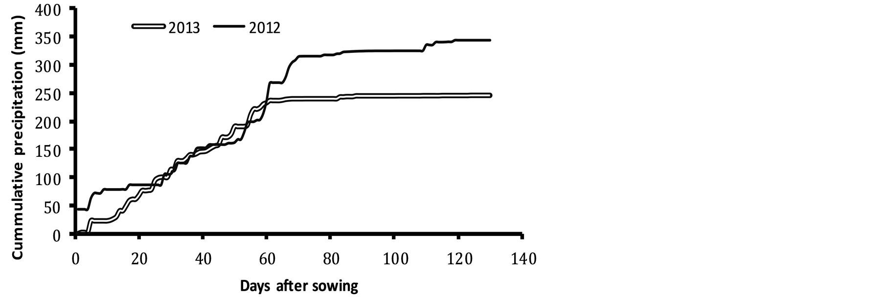
Figure 1. Cumulative precipitation for 2012 and 2013 growing seasons.
day after sowing) before crop establishment in which case supplemental irrigation was applied. During the 2013 season, dry spell was experienced towards the middle of the season just during silking and grain filling, so supplemental irrigation was also implemented.
Seasonal temperature and hence degree days between 2012 and 2013 seasons were not statistically different (P < 0.05) (Figure 2). However, total heat units received during 2013 season were slightly higher than those in the 2012 season. Regarding net solar radiation for the 2012 and 2013 growing seasons, pairwise t-test showed there was no significant difference (P = 0.1) between the seasons (Figure 3). Although there was no significant difference in weather elements between the two seasons, it was still important to test calibrate the model using two seasons since even the slightest difference matters for sound model calibration Soils within the study site and surroundings contain highly weathered clays and are highly acidic. Special management including drainage during heavy downpour or irrigation during dry spell was important due to higher clay contents. Due to acidity, phosphorus fixation was expected, hence phosphorus fertilizers were added.
3.2. Crop Growth and Development
3.2.1. Duration for Major Phenological Events
Although there was significant difference (P < 0.05) between varieties with respect to number of days to emergence and 50% anthesis, these phenological events did not differ significantly (P < 0.05) between 2012 and 2013 seasons. Days to physiological maturity between the seasons differed significantly (P = 0.002), 2013 season having more number of days to physiological maturity than the 2012 season. This was perhaps due the undetected stresses which occurred in 2013 but not in 2012. Although the experiments were conducted under as-
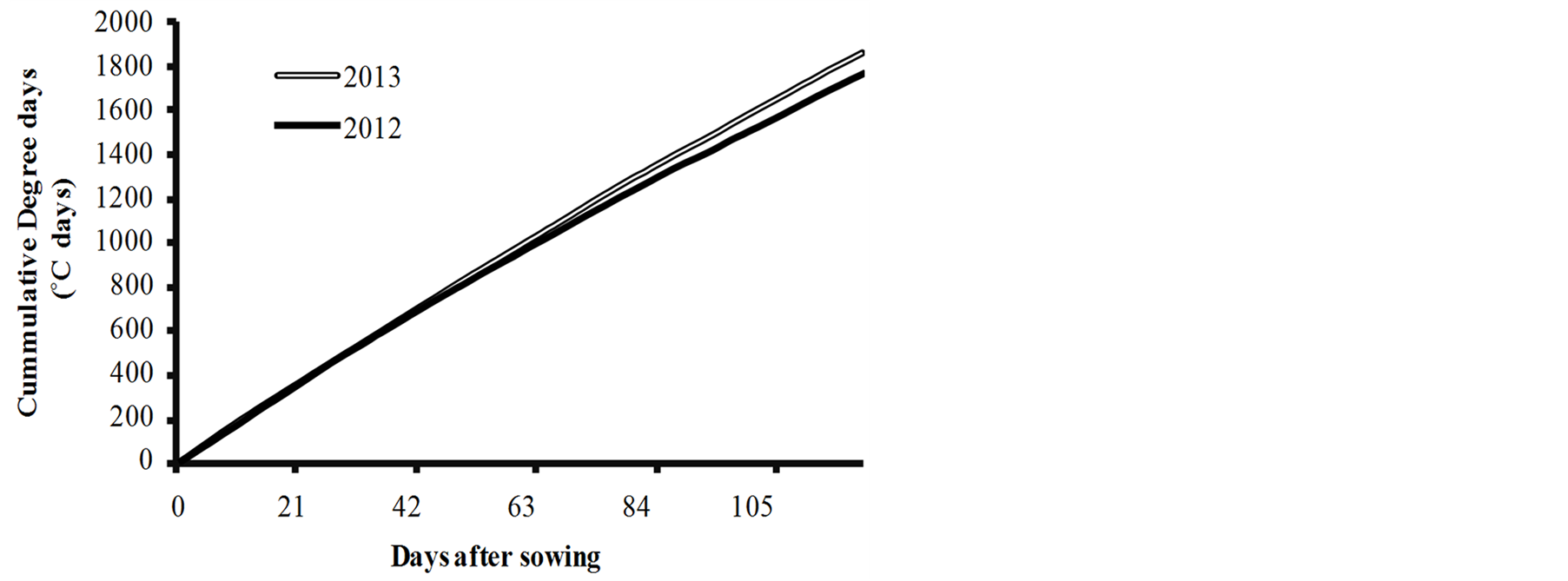
Figure 2. Cumulative thermal time for 2012 and 2013 growing seasons.
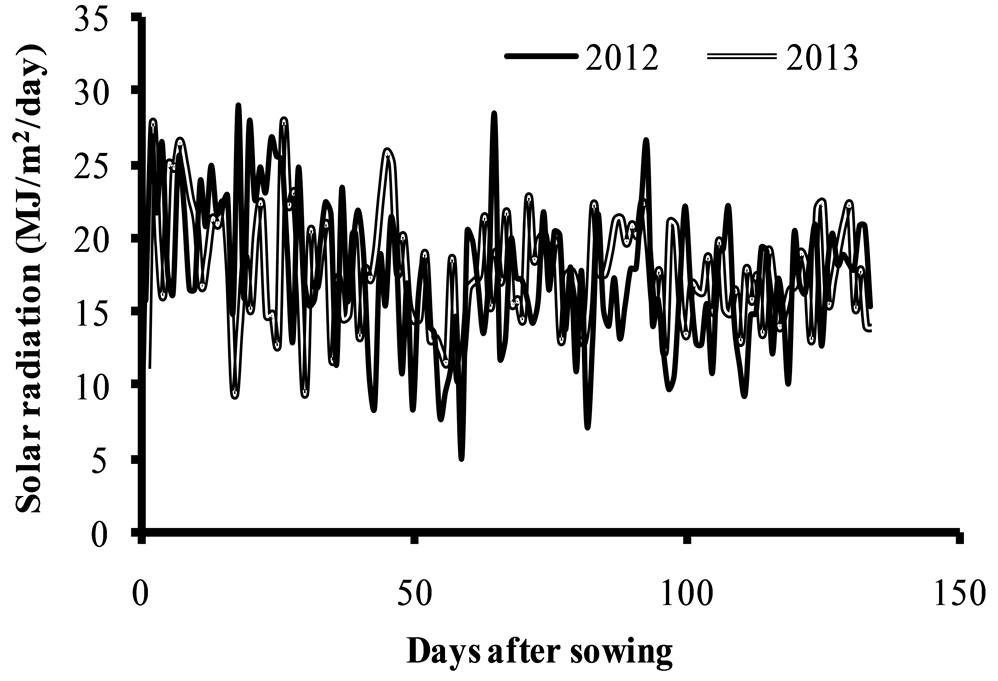
Figure 3. Net solar radiation for 2012 and 2013 growing seasons.
sumptions of optimality, it is often difficult to remove completely all stresses under field conditions.
3.2.2. Biomass and Yield
Except for the tops weight at physiological maturity which varied significantly (P < 0.05) during 2012 season, all other variables in did not vary. Likewise, there was no significant variation among varieties in the 2013 season with respect to biomass and yield (Table 4). Also, there was no inter seasonal variation in the tested variables of plant biomass at 50% anthesis, grain yield and tops weight at harvest as indicated by the t-statistic (Table 5).
The similarity in the parameters for the 2012 and 2013 growing seasons suggests that growing conditions of water, nutrient and other management were uniform across the seasons. For instance, the date of sowing for both seasons was the same, March, 08th, and because weather elements were more or less similar in both years, then the similarity could be anticipated.
3.2.3. CERES Maize Calibration
Observed and simulated days to anthesis and physiological maturity, grain yield, by-product biomass and total above-ground biomass converged for all cultivars (Tables 6 (a) and (b)), indicating that cultivar specific parameters within the model were reasonably adjusted. Also, there was a good relationship between observed and simulated variables (r2 values were respectively 0.96, 0.98, 1.0, 0.99 and 0.99 for days to anthesis, days to physiological maturity, grain yield, by-product biomass and total above-ground biomass). Stuka showed high RMSE with respect to both the number of days to anthesis and physiological maturity than others. TMV1 had higher RMSE with respect to grain yield and tops weight by 29% and 11% of the measured yield respectively The results indicate that Staha cultivar was high yielding and the yield is associated with the growth duration since it took longer than others to attain anthesis and physiological maturity.
3.2.4. Cultivar Specific Parameters
Results on cultivar specific parameters indicate that Stuka required few thermal units to complete juvenile stage (P1) when compared to Staha (Table 7). This allows Staha more time to accumulate photosynthates before silking, and hence higher yield in turn. Stuka which was originally bred for drought conditions indicates here that few heat units or short duration is just required to attain end of juvenile stage. This could be used as drought escaping mechanism, perhaps the breeders had in mind. Although Staha seems to give higher yields compared to other cultivars, it may be prone to water stress in case growing season is short due to dry spells towards the end. TMV1 required few heat units from anthesis to physiological maturity (P5), unlike Staha with highest thermal time requirement. Number of grains/ear (G2) also was high in Staha and lower in Pioneer. This corresponds
Table 4. F values for selected variables between maize cultivars for 2012 and 2013 seasons.
*significant at P < 0.05; ns = not significant.
Table 5. T-statistics for comparing 2012 and 2013 seasons with respect to selected variables.
ns = not significant at P < 0.05.
Table 6.Simulated and observed values for four maize cultivars. (a) Days to anthesis and days to maturity and grain yield (b) Byproduct yield and tops weight.
Table 7. Cultivar coefficients for the four maize varieties.
to differences in ear size between the two cultivars. The rate of grain development was high in Stuka as compared to other cultivars perhaps since this could be a drought avoidance mechanism for which this cultivar was developed. Phyllochron interval (PHINT) for the cultivars ranged from 30˚C days for TMV1 to 47.25˚C days for Staha.
There were no cultivar parameter values from the literature for comparing the values in this study. However, Tumbo et al. [26] estimated cultivar parameters for use in APSIM model. Thermal time to end of juvenile stage (P1) for Stuka was estimated to be 160˚C days whereas P5 was estimated to be 800˚C days. Difference between the values reported in this study and theirs could be that the parameters were merely estimated from little information available at that time e.g. days to tasseling, days to maturity and range of possible grain yields obtainable from varietal catalogue [27] , since growing conditions of soils, weather and management are not specified. This is one of the setbacks to estimate cultivar coefficients for modeling application or improvement in Tanzania because, while yield information may exist, there are no records for general crop growth conditions and on such aspects as planting dates, maturity dates, or total final biomass or initial field conditions.
As a way to applying DSSAT CSM in modeling maize yield in situations where specific cultivars are not known, a medium maturity generic cultivar (Cultivar code 990002) included in the DSSAT v4.5 cultivar database [8] is normally used ([10] [28] ). The cultivar specific parameters from this study are comparable to the mentioned generic cultivar in the DSSAT cultivar database. However, its use in model application in Tanzania requires a very careful consideration regarding the local spatial variations.
3.2.5. Model Evaluation
The cultivar specific parameters obtained from experiments reported above were used to evaluate CERES-Maize CSM for simulating different nitrogen treatments under rain-fed conditions. The model simulated well the average number of days to anthesis and maturity with high degree of agreement as indicated by the agreement index (d-statistics) (Table 8). This is an indication that the model calibration and resulting cultivar specific parameters were reasonably estimated. Generally there were significant differences (P < 0.05) between observed and simulated quantities at all nitrogen treatments and in all variables. Particularly, simulated yields increased consistently as N levels increased in both model simulations and experimental observations. This suggests that the CERES-Maize model is sensitive to environmental variables such as nutrient supply.
Grain yield for all varieties may not have been as high as that obtained in the calibration experiment due to water stress since evaluation experiment was carried out under rain dependent conditions. Also, plants under high nitrogen supply tend to face water stress since they have large leaf area from which more water loss takes place than in plants under sub optimal nutrient supply. Moreover t-test revealed significant difference (P < 0.05) between simulated and observed yields at all N levels (Table 9).
3.3. Sensitivity Analysis
Since phyllochron interval was difficult to measure under field conditions, sensitivity analysis was conducted by varying the PHINT values estimated from the model. By-product biomass was sensitive to changes in phyllochron (or the inverse of the rate of successive leaf tip appearance [29] (PHINT), being higher at low PHINT and vice versa (Figure 4). PHINT is critical in determining the duration of vegetative growth and in maize, it is lower in temperate but higher in tropical climate. Birch et al. [30] reported that phyllochron is influenced by temperature, increased by 1.7˚C day per ˚C increase in daily mean temperature when the latter increased from 12.5˚C to 25˚C prior to tassel initiation. From the results, it is apparent that by-product biomass was favoured by reduced phyllochron as a result of reduced daily mean temperature prior to tassel initiation. However, other environmental variables such as nitrogen [31] have been reported to affect the phyllochron.
Furthermore, reduced phyllochron means that crops’ vegetative stages would take longer time and thus accumulated more photosynthates than they would in increased phyllochron as is the case when plants are grown in
Table 8. Observed and simulated values for variables as affected by three nitrogen levels under rainfed conditions. Values in parentheses indicate standard deviation (n = 12).
Table 9. Simulated vs. observed grain yields at different nitrogen levels. Values in parentheses indicate standard deviation for the observed treatment effects.
high temperatures or other environmental stresses.
A ten per cent decrease in PHINT only resulted in yield increase for Stuka cultivar while at 5% less, the yield increased significantly (Figure 5). For other cultivars, decreasing or increasing PHINT resulted into reduced yields with significant variation among them. The variation among cultivars was perhaps due to the genetic differences, indicating that some cultivars such as Stuka can perform better in environments with aspects which reduce PHINT (increase rate of leaf appearance) than those which increase PHINT (reduce rate of leaf appearance) (Figure 5). For such varieties as TMV1 and Pioneer seem to have adapted range of environmental variables below or above which PHINT affects grain yield. The yield reduction was more pronounced when PHINT was increased by 10% from normal, implying that leaf appearance rate would be below permissible limits, leading to yield decline. This can be used to explain why crops grown under stressful conditions of water or nutrients which affects leaf appearance rate give low yields. Generally, the model sensitivity may indicate that cultivars used in this study are adapted to environments which favour moderate leaf appearance rate, not too cold (where temperature reduces PHINT or too hot where higher temperature increases PHINT.
4. Conclusion
Lack of experimental data on locally adapted maize cultivars has hindered a great deal DSSAT CSM application in various areas, such as biophysical resource utilization, or efficient and cost effective tactical or strategic decision making processes and research. In this study, the maize cultivar specific parameters were quantified for four, medium maturing low land maize cultivars. Simulation experiments done using these cultivar parameters predicted reasonably well the crop growth and yield under varying nitrogen management conditions. The parameter PHINT which was difficult to measure under field conditions was roughly within the published range. However, careful measurements perhaps in a growth chambers is warranted to determine its values for the maize cultivars used. Within the limits of experimental conditions under which the cultivar parameters were quantified, it is concluded therefore that these cultivar parameters can be validly used in the DSSAT CSM application for
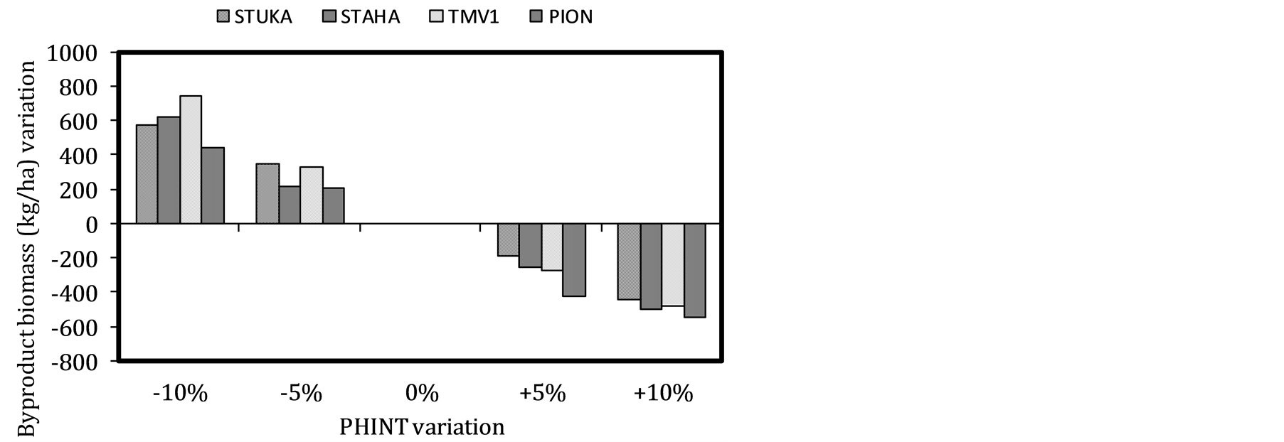
Figure 4. Changes in by-product biomass due to variation in PHINT.
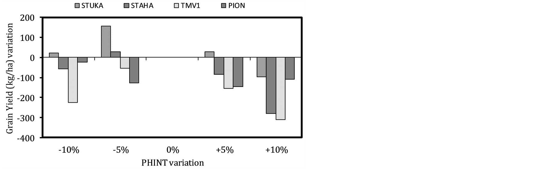
Figure 5. Changes in grain yield due to variation in PHINT.
the cultivars used.
Acknowledgements
This study was generously funded by the Alliance for Green Revolution in Africa (AGRA—Soil Health Program), Agricultural Model Inter-comparison and Improvement Project (AgMIP) and Enhancing Climate Change Adaptation in Agriculture and Water Resources (ECAW) Project.
References
- van Ittersum, M.K., Cassman, K.G., Grassini, P., Wolfa, J., Tittonell, P. and Hochmand, Z. (2013) Yield Gap Analysis with Local to Global Relevance—A Review. Field Crops Research, 143, 4-17. http://dx.doi.org/10.1016/j.fcr.2012.09.009
- Rosenzweig, C. and Liverman, D. (1992) Predicted Effects of Climate Change on Agriculture: A Comparison of Temperate and Tropical Regions. In: Majumdar, S. K., Ed., Global Climate Change: Implications, Challenges, and Mitigation Measures, The Pennsylvania Academy of Sciences, PA, 342-361.
- White, J.W., Hoogenboom, G., Kimball, B.A. and Wall, G.W. (2011) Methodologies for Simulating Impacts of Climate Change on Crop Production. Field Crops Research, 124, 357-368. http://dx.doi.org/10.1016/j.fcr.2011.07.001
- Mupangwa, W., Dimes, J., Walker, S. and Twomlow, S. (2011) Measuring and Simulating Maize (Zea mays L.) Yield Responses to Reduced Tillage and Mulching under Semi-Arid Conditions. Agricultural Sciences, 2, 167-174. http://dx.doi.org/10.4236/as.2011.23023
- MAFSC (2013) Agricultural Basic Data 2005/2006-2009/2010. http://www.kilimo.go.tz/agricultural/statistics/Basic/Chapter4.pdf
- FAOSTAT, (2012) Food and Agricultural Commodities Production. http://faostat.fao.org/site/339/default.aspx
- Hunt, L.A. and Boote, K.J. (1998) Data for Model Operation, Calibration and Evaluation. In: Tsuji, G.Y., Hoogenboom, G. and Thornton, P.K., Eds., Understanding Options for Agricultural Production, Kluwer Academic Publishers/ICASA, Dordrecht, 9-40.
- Hoogenboom, G., Jones, J.W., Wilkens, P.W., Porter, C.H., Boote, K.J. and Hunt, L.A. (2010) Decision Support System for Agrotechnology Transfer (DSSAT) Version 4.5, Honolulu, University of Hawai, CD ROM.
- Mwandosya, M.J., Nyenzi, B.S. and Luhanga, M.L. (1998) The Assessment of Vulnerability and Adaptation to Climate Change Impacts in Tanzania. Centre for Energy, Environmental Science and Technology, Dar-es-Salaam, Tanzania.
- Harvest Choice (2010) Yield Gap: Rain-fed Maize. IFPRI, Washington, http://harvestchoice.org/node/1622
- Arndt, C., Farmer, W., Strzepek, K. and Thurlow, J. (2011) Climate Change, Agriculture and Food Security in Tanzania. Working Paper No. 6188. United Nations University-World Institute for Economic Development Research (UNU-WIDER), 26.
- Anothai, J., Patanothai, A., Jogloy, S., Pannangpetch, K., Boote, K.J. and Hoogenboom, G. (2008) A Sequential Approach for Determining the Cultivar Coefficients of Peanut Lines Using End-Of-Season Data of Crop Performance Trials. Field Crops Research, 108, 169-178. http://dx.doi.org/10.1016/j.fcr.2008.04.012
- Bannayan, M. and Hoogenboom, G. (2009) Using Pattern Recognition for Estimating Cultivar Coefficients Of a Crop Simulation Model. Field Crops Research, 111, 290-302. http://dx.doi.org/10.1016/j.fcr.2009.01.007
- He, J., Jones, J.W., Graham, W.D. and Dukes, M.D. (2010) Influence of Likelihood Function Choice for Estimating Crop Model Parameters Using the Generalized Likelihood Uncertainty Estimation Method. Agricultural Systems, 103, 256-264. http://dx.doi.org/10.1016/j.agsy.2010.01.006
- MacCarthy, D.S., Vlek, P.L.G. and Fosu-Mensah, B.Y. (2012) The Response of Maize to N Fertilization in a Sub-Humid Region of Ghana: Understanding the Process Using a Crop Simulation Model. In: Kihara, J., Fatondji, D., Jones, J. W., Hoogenboom, G., Tabo, R. and Bationo, A., Eds., Improving Soil Fertility Recommendations in Africa using the Decision Support System for Agrotechnology Transfer (DSSAT), Springer Science + Business Media, Dordrecht, 61-75.
- Jones, P.G. and Thornton, P.K. (2003) The Potential Impacts of Climate Change on Maize Production in Africa and Latin America in 2055. Global Environmental Change, 13, 51-59. http://dx.doi.org/10.1016/S0959-3780(02)00090-0
- Craufurd, P.Q., Vadez, V., Jagadish, S.V.K., Vara-Prasad, P.V. and Zaman-Allah, M. (2013) Crop Science Experiments Designed to Inform Crop Modeling. Agricultural and Forest Meteorology, 170, 8-18. http://dx.doi.org/10.1016/j.agrformet.2011.09.003
- Jones, C.A. and Kiniry, J.R. (1986) CERES-Maize. Texas A&M University Press, College Station.
- Jones, J.W., Hoogenboom, G., Porter, C.H., Boote, K.J., Batchelor, W.D., Hunt, L.A., Wilkens, P.W., Singh, U., Gijsman, A.J. and Ritchie, J.T. (2003) The DSSAT Cropping System Model. European Journal of Agronomy, 18, 235-265. http://dx.doi.org/10.1016/S1161-0301(02)00107-7
- Hoogenboom, G., Jones, J.W., Traore, P.C.S. and Boote, K.J. (2012) Experiments and Data for Model Evaluation and Application. In: Kihara, J., Fatondji, D. Jones, J.W., Hoogenboom, G., Tabo, R. and Bationo, A., Eds., Improving Soil Fertility Recommendations in Africa Using the Decision Support System for Agrotechnology Transfer (DSSAT), Springer Science + Business Media, Dordrecht, 9-18.
- Mokhtarpour, H., Teh, C.B.S., Saleh, G., Selamat, A.B., Asadi, M.E. and Kamkar, B. (2010) Non-Destructive Estimation of Maize Leaf Area, Fresh Weight, and Dry Weight Using Leaf Length and Leaf Width. Communications in Biometry and Crop Science, 5, 19-26.
- Ogoshi, R.M., Cagauan, B.G. and Tsuji, G.Y. (1999) Field and Laboratory Methods for Collection of Minimum Data sets. In: Hoogenboom, G., Wilkens P.W. and Tsuji G.Y., Eds., DSSAT, Version 3, Vol. 4. IBSNAT-ICASA, University of Hawaii, Honolulu, 217-286.
- United Republic of Tanzania (1993) Review of Fertilizer Recommendation in Tanzania. Soil Fertility Report F6, National Soil Service, Tanga, Tanzania.
- Wallach, D. (2006) Evaluating Crop Models. In: Wallach, D., Makowski, D. and Jones, J.W., Eds., Working with Dynamic Crop Models Evaluation, Analysis, Parameterization, and Applications, Elsevier, Amsterdam, 11-54.
- Wilmott, C.J. (1981) On the Validation of Models. Physical Geography, 2, 184-194.
- Tumbo, S.D., Kahimba, F.C., Mbilinyi, B.P., Rwehumbiza, F.B., Mahoo, H.F., Mbungu, W.B. and Enfors, E. (2012) Impact of Projected Climate Change on Agricultural Production in Semi-Arid Areas of Tanzania: A Case of Same District. African Crop Science Journal, 20, 453-463.
- MAFSC (2012) Tanzania Variety Catalogue. http://www.kilimo.go.tz/publications/publications.htm
- Cenacchi, N. and Koo, J. (2011) Effects of Drought Tolerance on Maize Yield in Sub-Saharan Africa. http://addis2011.ifpri.info/files/2011/10/Paper_4C_Nichola-Cenacci.pdf
- Tollenaar, M. and Lee, E.A. (2002) Yield Potential Yield, Yield Stability and Stress Tolerance in Maize. Field Crops Research, 75, 161-170. http://dx.doi.org/10.1016/S0378-4290(02)00024-2
- Birch, C.J., Vos, J., Kiniry, J., Bos, H.J. and Elings, A. (1998) Phyllochron Responds to Acclimation to Temperature and Irradiance in Maize. Field Crops Research, 59, 187-200. http://dx.doi.org/10.1016/S0378-4290(98)00120-8
NOTES

*Corresponding author.