Open Journal of Air Pollution
Vol.1 No.2(2012), Article ID:23188,9 pages DOI:10.4236/ojap.2012.12006
Studies on Interrelations among SO2, NO2 and PM10 Concentrations and Their Predictions in Ambient Air in Kolkata
1Department of Environmental Studies, Women’s Christian College, Kolkata, India
2Department of Environmental Science, Asutosh College, Kolkata, India
3Department of Mathematics and Post Graduate Department of Environmental Science, Asutosh College, Kolkata, India
Email: phalguni.mukherjee@gmail.com
Received July 10, 2012; revised August 19, 2012; accepted September 11, 2012
Keywords: Ambient Air; Multiple Correlation-Coefficients; Kolkata
ABSTRACT
In this paper we have first of all studied the interrelations among the concentrations of SO2, NO2 and PM10 and then predicted their future level of concentrations in the ambient air of Kolkata. The data collected from West Bengal Pollution Control Board website have been used to construct second degree, third degree and four degree polynomial equations using MATLAB software. Since a curve in a small interval can be approximated by a line segment in that small interval, we have observed that better result can be achieved if we replace the curves piece meal wise in small intervals by line segments during January-April, May-August and September-December months. The multiple regression equations among the aforesaid three parameters have been established to predict the value of each parameter in terms of the remaining two. A further improvement in terms of reducing the number of dependent variables has been made using the results of correlation coefficients. Finally, we have predicted the value of each parameter in terms of only one dependent variable.
1. Introduction
Metropolitan city like Kolkata has been suffering from various types of health hazards problems for long time due to air pollution. Risk assessments for the toxic pollutants are widely used in different countries as a regulatory decision making processes to combat air pollution [1]. In the mega cities of India such as Mumbai, Delhi and Kolkata, PM10 has exceeded the regulatory limits [2,3]. It has been found from available data that the presence of particulate matter (PM10) is highest in the atmosphere of Kolkata. Among the pollutants listed in NAAQS [4] one of the most notorious pollutants is PM10. It is well known that PM10 is responsible for respiratory hazards in human health. Such particulates can also obstruct lung function without reacting chemically, by depositing in human lungs and interfering with normal functioning [5]. Moreover, it takes part in formation of sulphurous smog. One of the main sources of existence of PM10 in air is vehicular pollution. Various typical anthropogenic activities like intense transportation, Industrial and commercial activities are prevailing in urban areas, particularly in the metropolitan cities [1,6-8]. It is also known that increased level of Sulphur-dioxide (SO2) and Nitrogen-dioxide (NO2) lead to the formation of different types of secondary pollutants in environment. Studies reveal that the occurrence is mainly due to expanding industries and growing number of vehicles within the state. The West Bengal Pollution Control Board (WBPCB) had initiated air quality monitoring of Kolkata through a limited number of stations in 1992 and subsequently expanded its monitoring network to systematic pattern from December 1998 [9]. At present the air quality of Kolkata is monitored through 16 fixed monitoring stations as mentioned in Methods and Materials.
2. Objective
Our main objective is to study the interrelations among the concentrations of SO2, NO2 and PM10, and to use these results to predict each of these three pollutants in the city of Kolkata. We have used MATLAB software on the available data to suitably fit second degree, third degree and fourth degree curves for each parameter. It has been found that the best predictions for some of the parameters are obtained sometimes for second degree, sometimes for third degree and sometimes for fourth degree curves—but no unique curve is obtained to make best predictions for all the three parameters. Since a curve in a small interval can be approximated by a line segment in that small interval, we have considered the curves piece meal wise from January to April, May to August and September to December for all the parameters. Then we have approximated the curves obtained in the above time periods by suitable line segments and found predictions are quite encouraging. Next we find multiple regression equations among PM10, SO2 and NO2 and predict the approximate value of one of the parameters in terms of remaining two. Further, we have found out the correlation between each pair of parameters and used these results to reduce the number of dependent variables from two to one and predict any one of the parameters in terms of only one (dependent) parameter.
3. Methods and Materials
The average value of 24 hr daily ambient air quality information has been collected during the period of 2003- 2010 for all three pollutants and subsequently their monthly averages have been obtained for each of these pollutants (Tables 1-3).
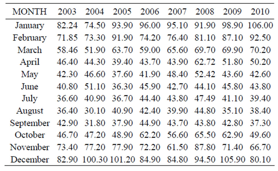
Table 1. The average month wise data for NO2 (Source: Daily Ambient Air quality Information [10]; WBPCB) in terms of (µg/m³).
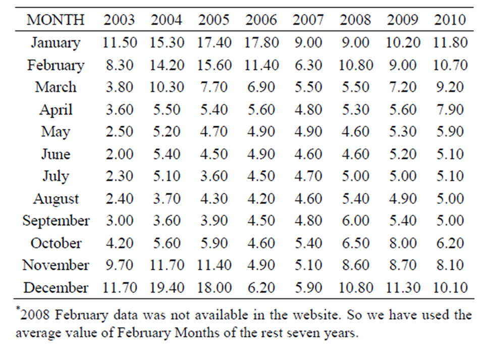
Table 2. The average month wise data for SO2 (Source: Daily Ambient Air quality Information [10]; WBPCB) in terms of (µg/m³).
Study Area
Study area selected by WBPCB includes 16 stations in the city Kolkata, they are at Dunlop Bridge, Picnic Garden, Tollygunge, Hyde Road, Behala Chowrasta, Beliaghata, Salt Lake, Tapsia, Baishnabghata, Ultadanga, Mominpore, Moulali, Shyambazar, Gariahat, Minto Park, Rajarhat New Township.
4. Results and Discussion
These primary data have been used to get non-linear curve for each case. We then use MATLAB to predict their concentrations by second degree, third degree and fourth degree equation (Tables 4-12).
The results thus obtained are quite good except in a few cases. So for obtaining better result in terms of accuracy, we have again divided the entire data into three segments i.e. from January-April, May-August and September-December. In each case we get linear equations (Figures 1-9) and the predictions made are quite encouraging.

Table 3. The average month wise data for PM10 (Source: Daily Ambient Air quality Information [10]; WBPCB) in terms of (µg/m³).
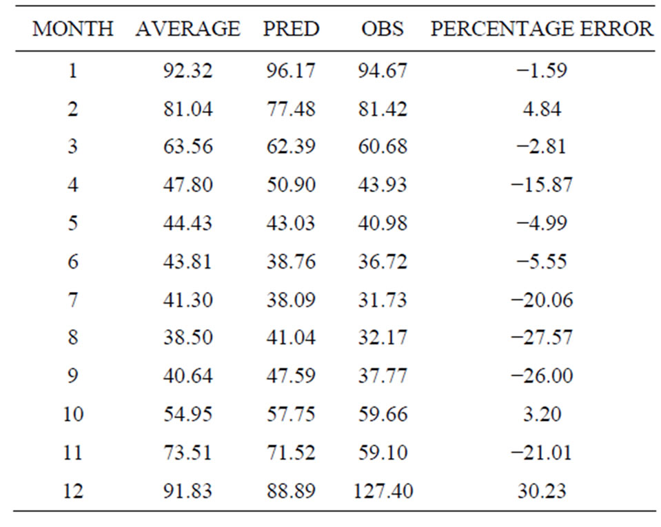
Table 4. Prediction of NO2 using second degree equation.
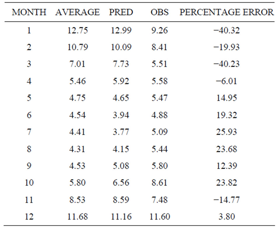
Table 5. Prediction of SO2 using second degree equation.
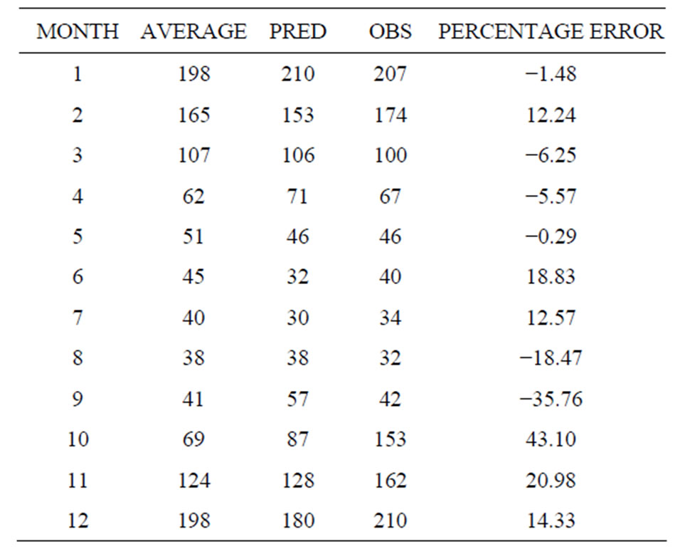
Table 6. Prediction of PM10 using second degree equation.
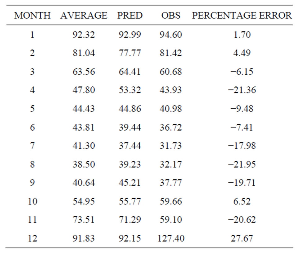
Table 7. Prediction of NO2 using third degree equation.
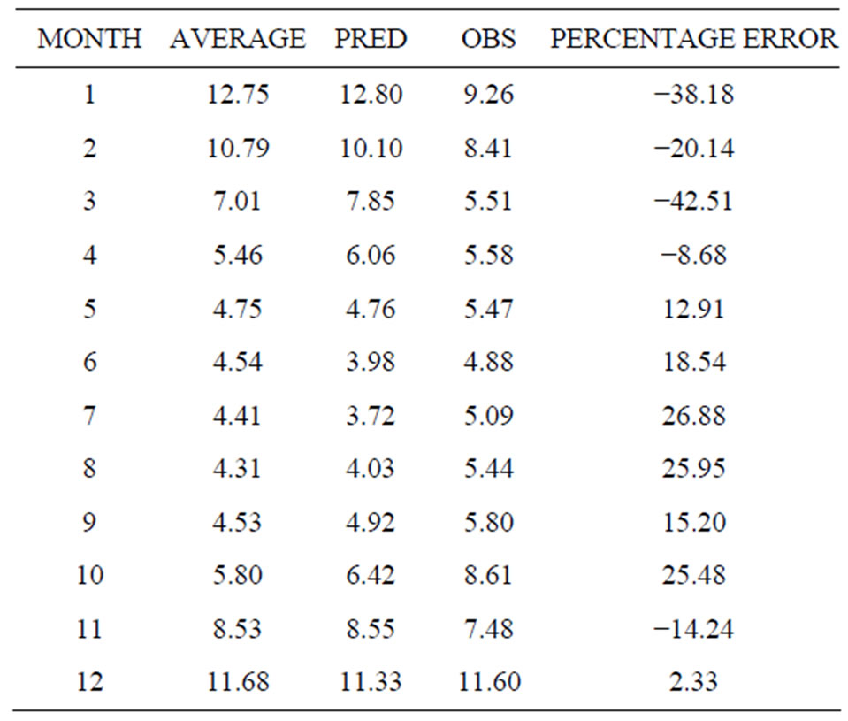
Table 8. Prediction of SO2 using third degree equation.
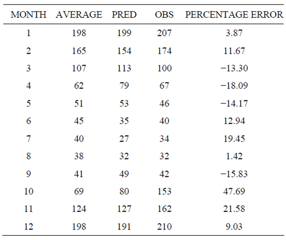
Table 9. Prediction of PM10 using third degree equation.
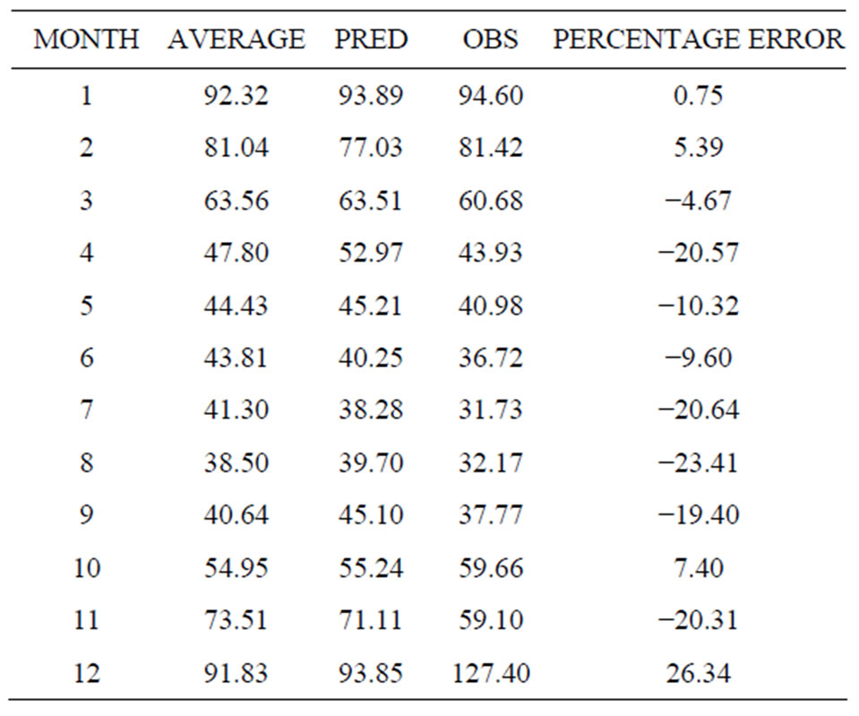
Table 10. Prediction of NO2 using fourth degree equation.
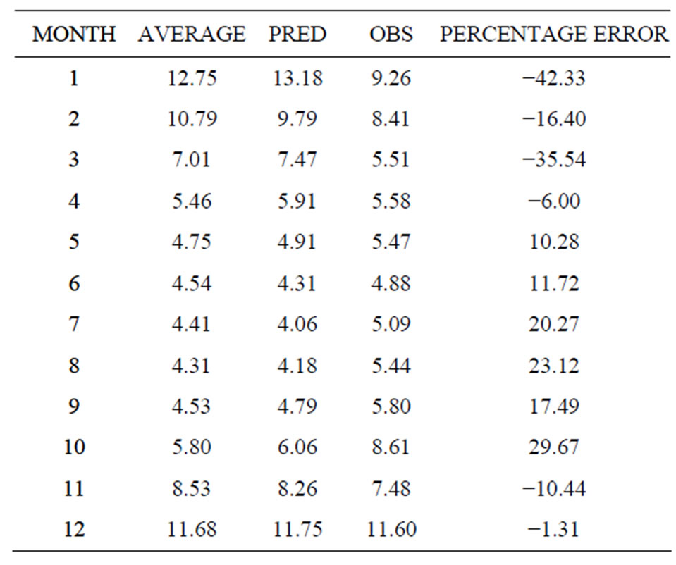
Table 11. Prediction of SO2 using fourth degree equation.
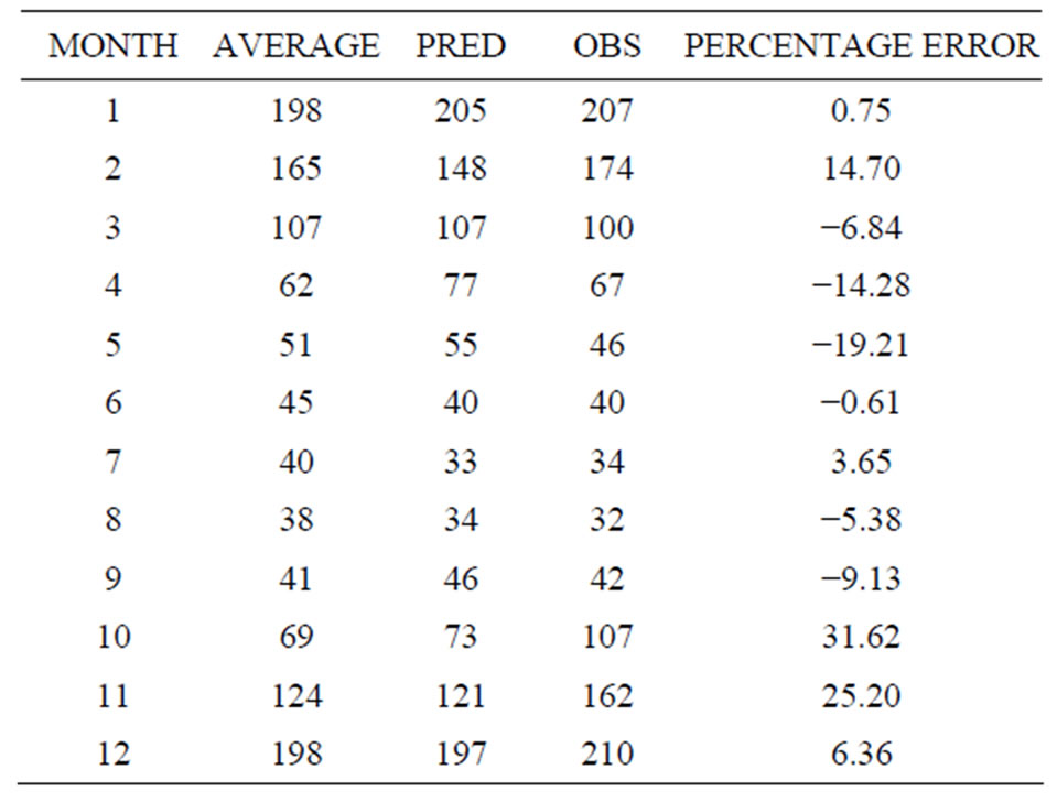
Table 12. Prediction of PM10 using fourth degree equation.
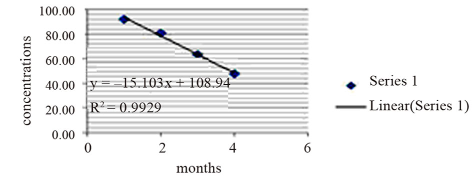
Figure 1. Linear equation of NO2 during January-April.
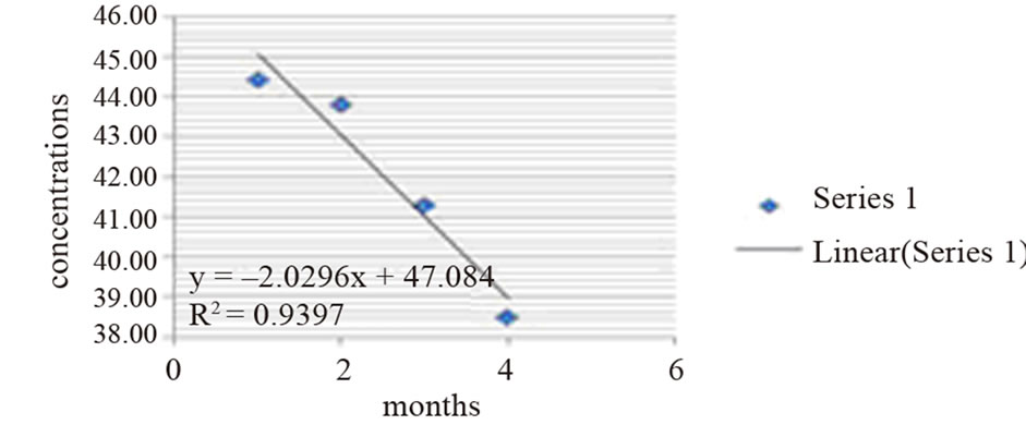
Figure 2. Linear equation of NO2 during May-August.
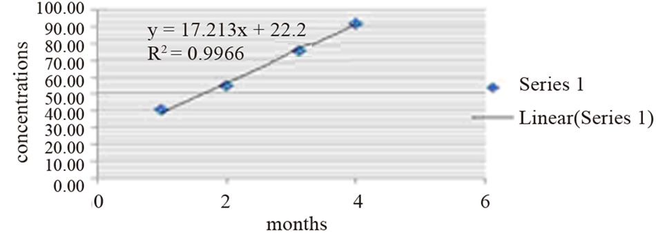
Figure 3. Linear equation of NO2 during September-December.
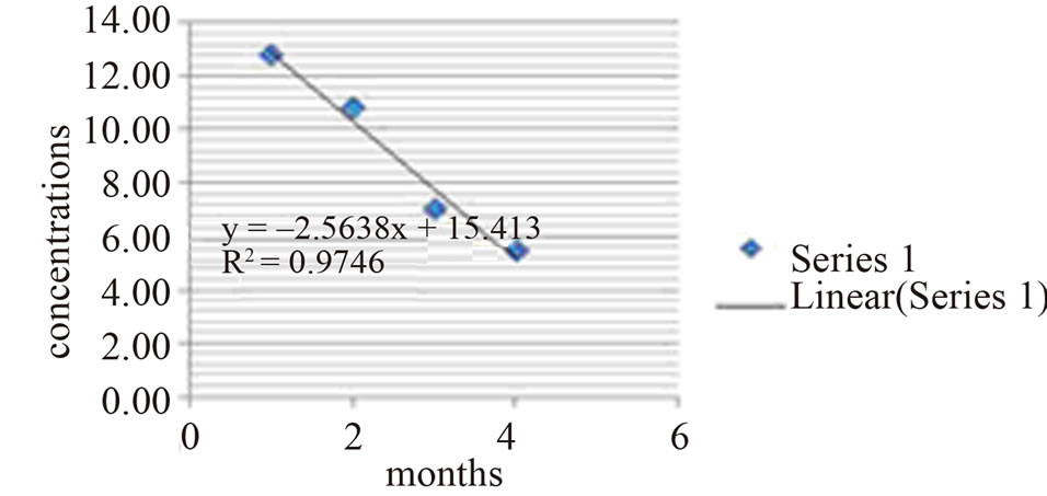
Figure 4. Linear equation of SO2 during January-April.
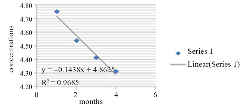
Figure 5. Linear equation of SO2 during May-August.
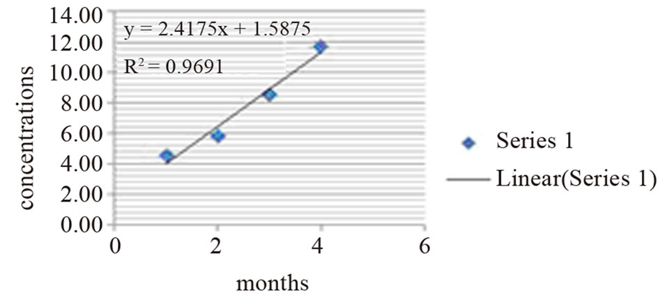
Figure 6. Linear equation of SO2 during September-December.
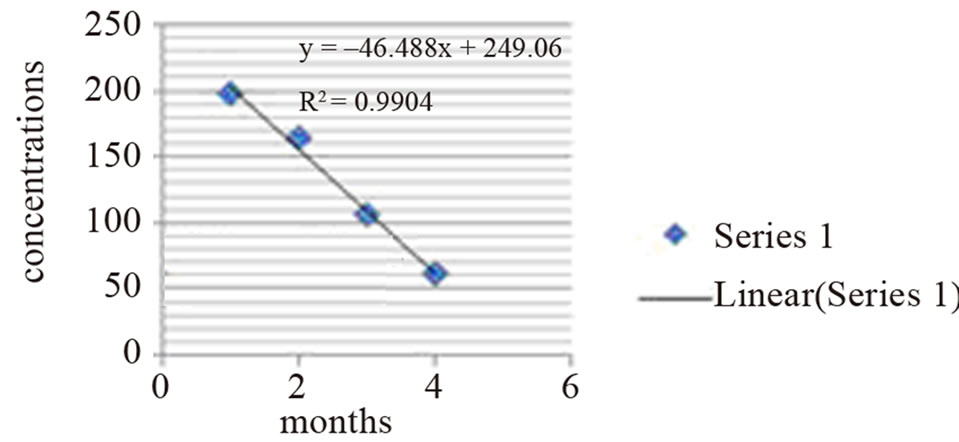
Figure 7. Linear equation of PM10 during January-April.
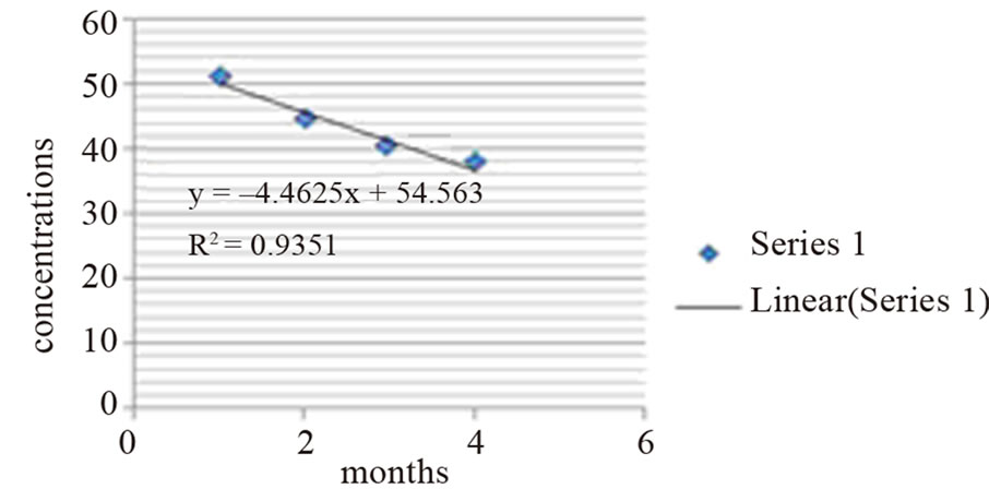
Figure 8. Linear equation of PM10 during May-August.
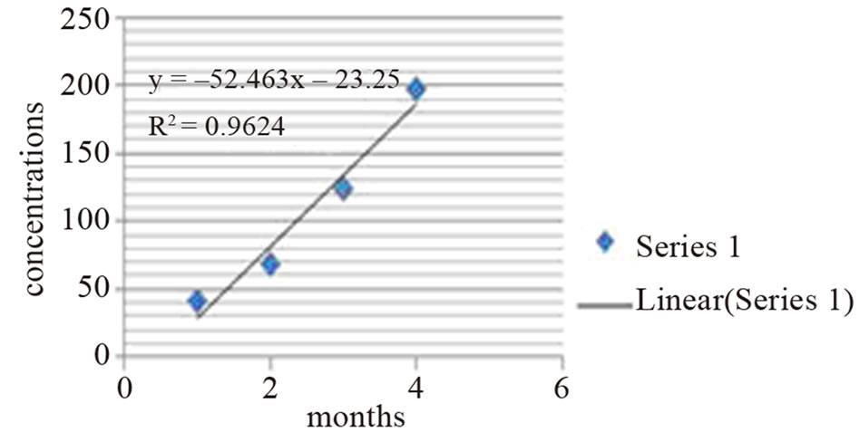
Figure 9. Linear equation of PM10 during September-December.
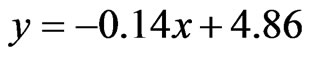
The prediction of NO2 during January-April is given by the equation
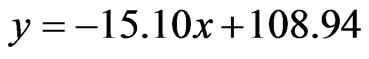 (1)
(1)
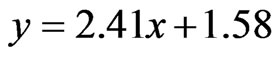
The prediction of NO2 during May-August is given by the equation
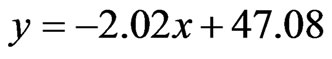 (2)
(2)
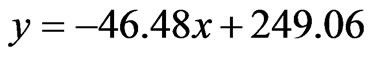
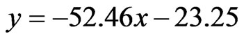
The prediction of NO2 during September-December is given by the equation
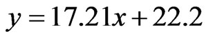 (3)
(3)
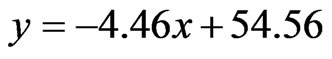
The prediction of SO2 during January-April is given by the equation
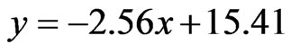 (4)
(4)
The prediction of SO2 during May-August is given by the equation
 (5)
(5)
The prediction of SO2 during September-December is given by the equation
 (6)
(6)
The prediction of PM10 during January-April is given by the equation
 (7)
(7)
The prediction of PM10 during May-August is given by the equation
 (8)
(8)
The prediction of PM10 during September-December is given by the equation
 (9)
(9)
Results obtain from line segments are tabulated as (Tables 13-15).
Explanation of data given in Table 13: NO2: Average values of NO2 during 2003-2010; PRED: Predicted value of NO2 obtained from Figures 1-3; OBS: Month wise observed values of 2011.
Explanation of data given in Table 14: SO2: Average values of SO2 during 2003-2010; PRED: Predicted value of SO2 obtained from Figures 4-6; OBS: Month wise observed values of 2011.
Explanation of data given in Table 15: PM10: Average values of PM10 during 2003-2010; PRED: Predicted value of PM10 obtained from Figures 7-9; OBS: Month wise observed values of 2011.
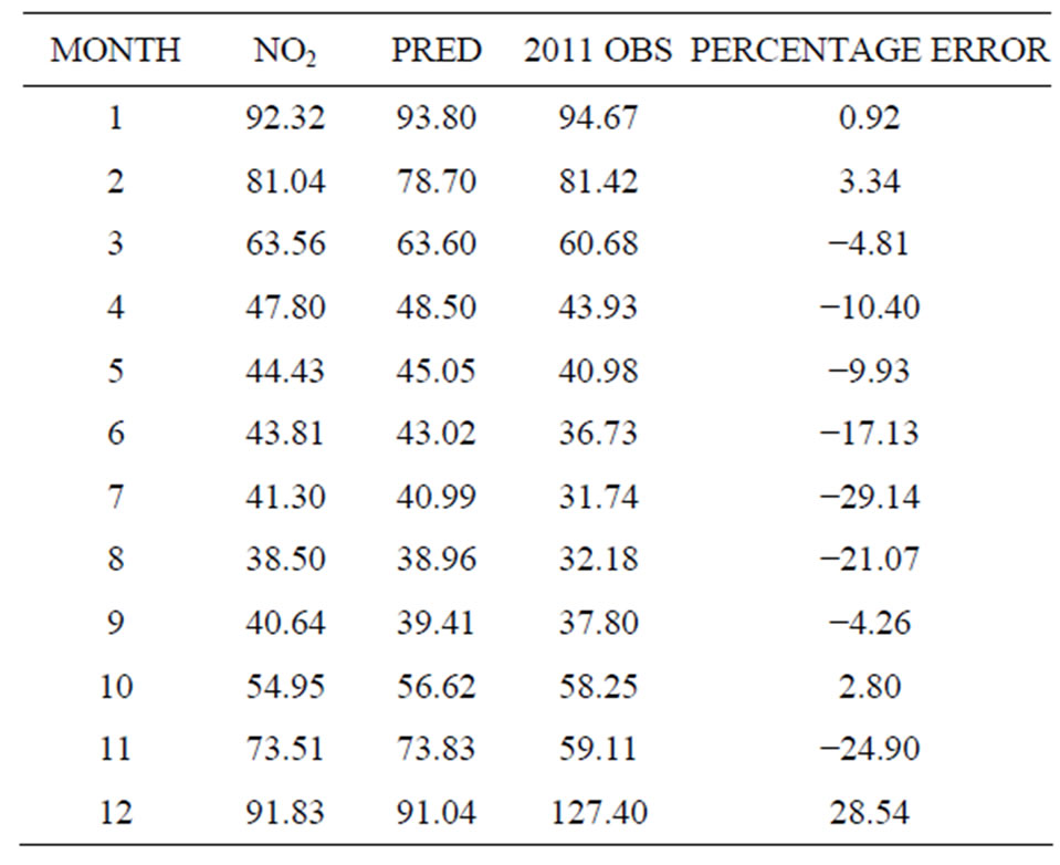
Table 13. Prediction of NO2.
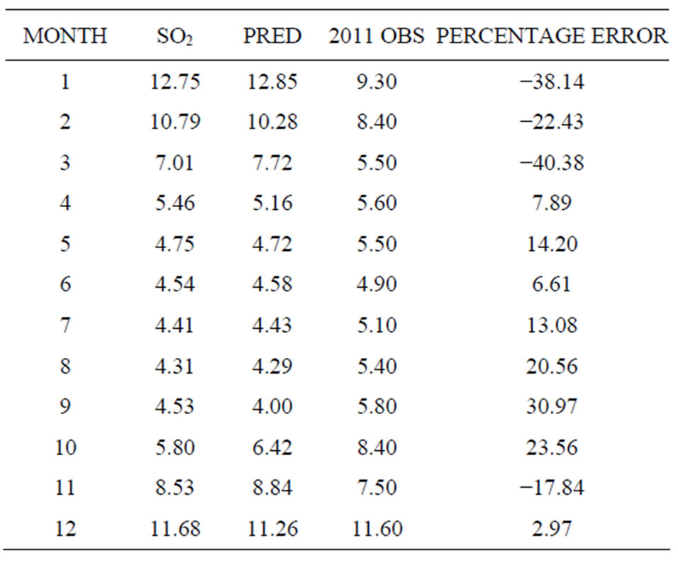
Table 14. Prediction of SO2.
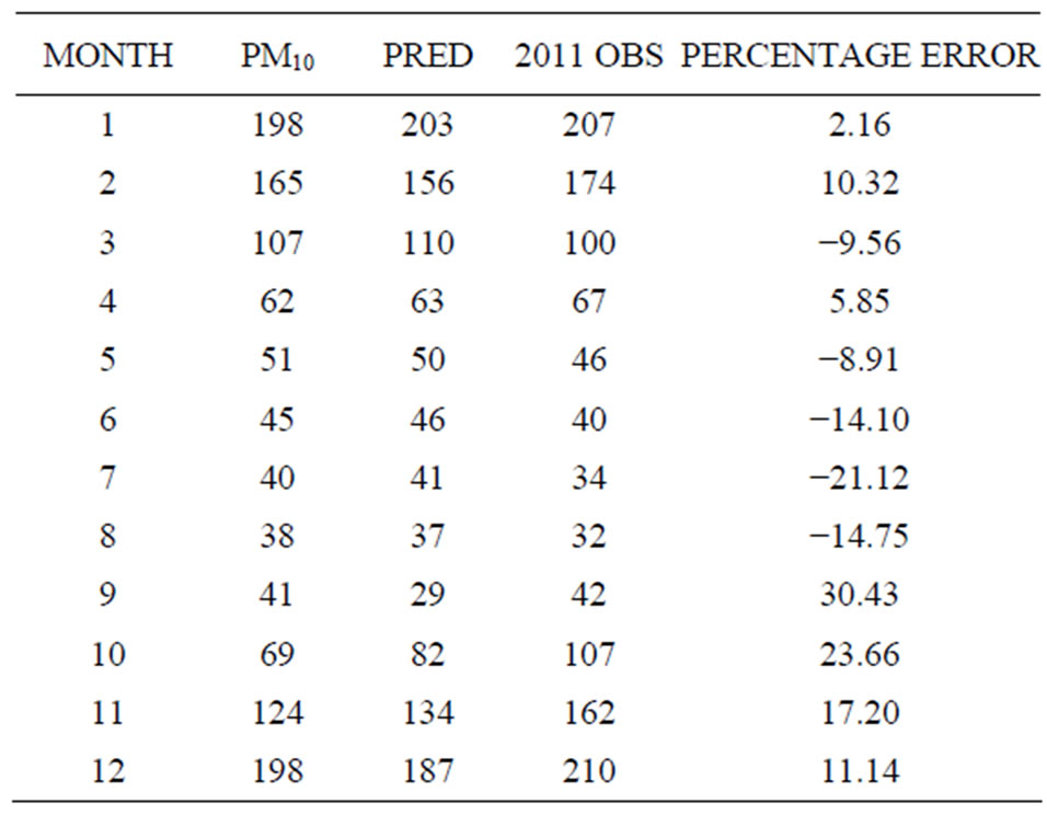
Table 15. Prediction of PM10.
We have divided the entire data into three segments, for each segment we have established a multiple regression equation involving all the three parameters. The segment-wise equations are as follows:
January-April: 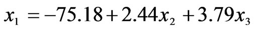 (10)
(10)
May-August: 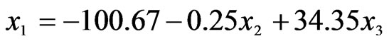 (11)
(11)
September-December:
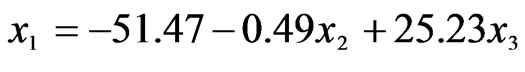 (12)
(12)
The results obtain from the above three equations are shown in Table 16.
Next we consider the average values of NO2, SO2 and PM10 from January-April, during 2003-2010 to find linear relations between every pair of parameters. The results for all the segments are shown in the following figures and tables.
The correlation co-efficient of each of the three parameters during January-April, May-August, September-December are shown in Tables 17-19 and Figures 10-18 respectively.
 (13)
(13)
 (14)
(14)
 (15)
(15)
 (16)
(16)
 (17)
(17)
 (18)
(18)
 (19)
(19)
 (20)
(20)
 (21)
(21)
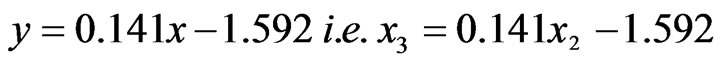
In the following table we have shown linear relations between every pair of parameters for all the three segments.
From Table 16 and Table 20 we put together the results in Table 21 where we have predicted each parameter.
1) In terms of remaining two parameters;
2) In terms of one of the remaining parameters.
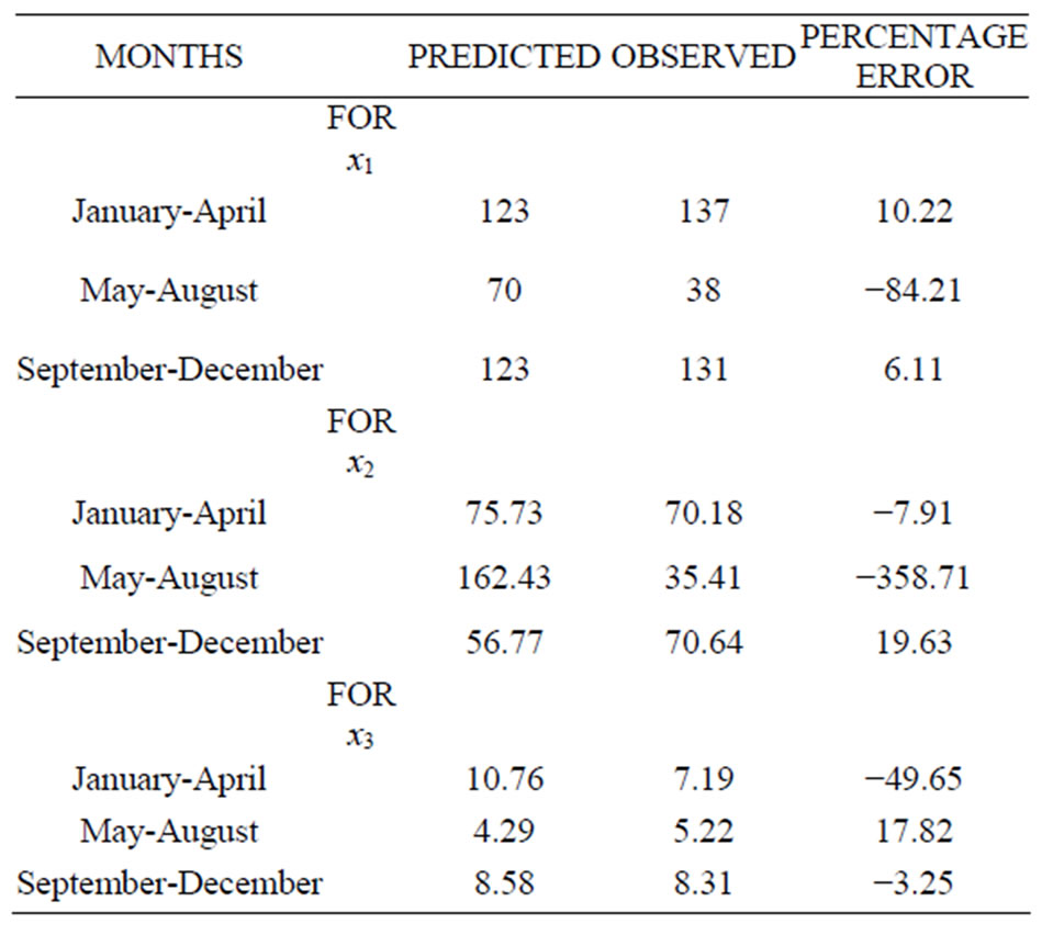
Table 16. Prediction of x1, x2 and x3 with the help of multiple regression equations involving all the parameters during the segments (January-April, May-August, and SeptemberDecember).
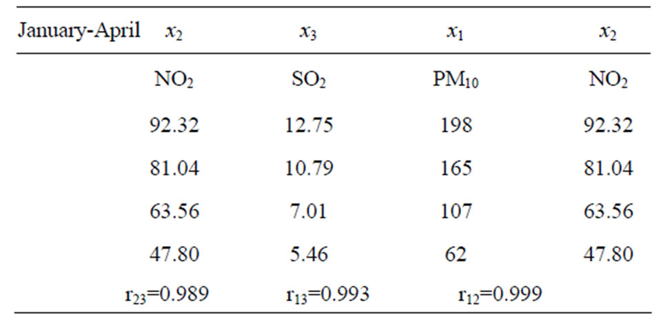
Table 17. Correlation co-efficient of each three parameters during January-April.
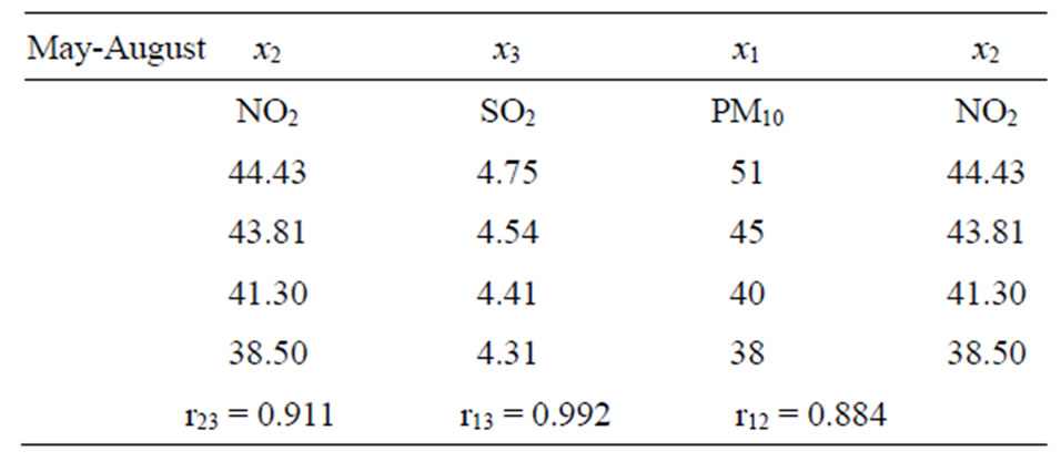
Table 18. Correlation co-efficient of each three parameters during May-August.
For all the three segments a mentioned earlier, we have also calculated errors in each case.
If we study the above data, it is interesting to observe that the prediction of PM10 (x1) concentration is more accurate when we use known concentration of NO2 (x2) only (i.e. x1 gives the best result when x1 = f(x2) is considered). Again using known PM10 concentration the more accurate value of NO2 can be measured during January to August. For last segment less error for prediction of NO2 has been encountered when known SO2 concentration is used. From the following table we can find the minimum errors for prediction of each parameter during different segments.
Season-wise identification of dependent variable to predict each parameter with minimum error are given in Table 22.
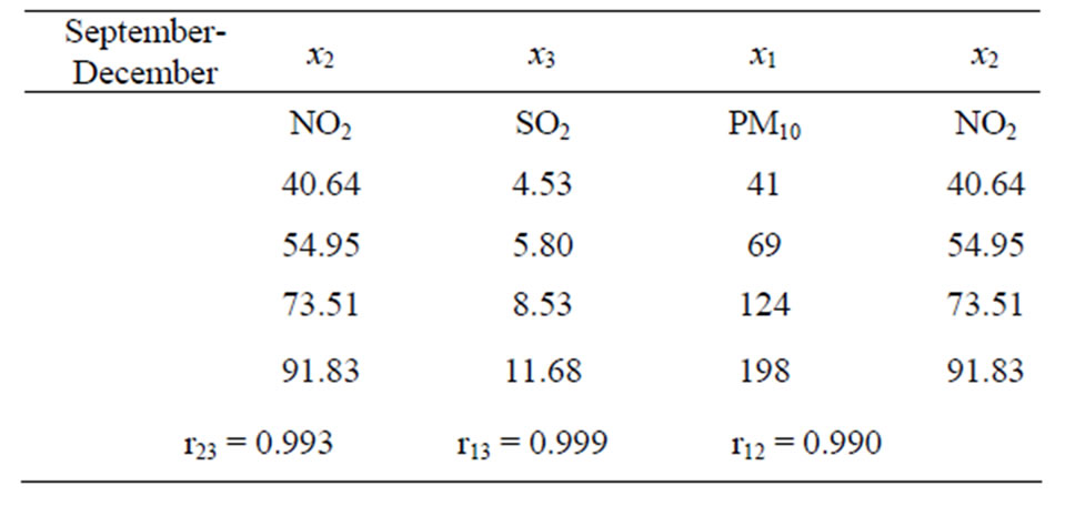
Table 19. Correlation co-efficient of each three parameters during September-December.
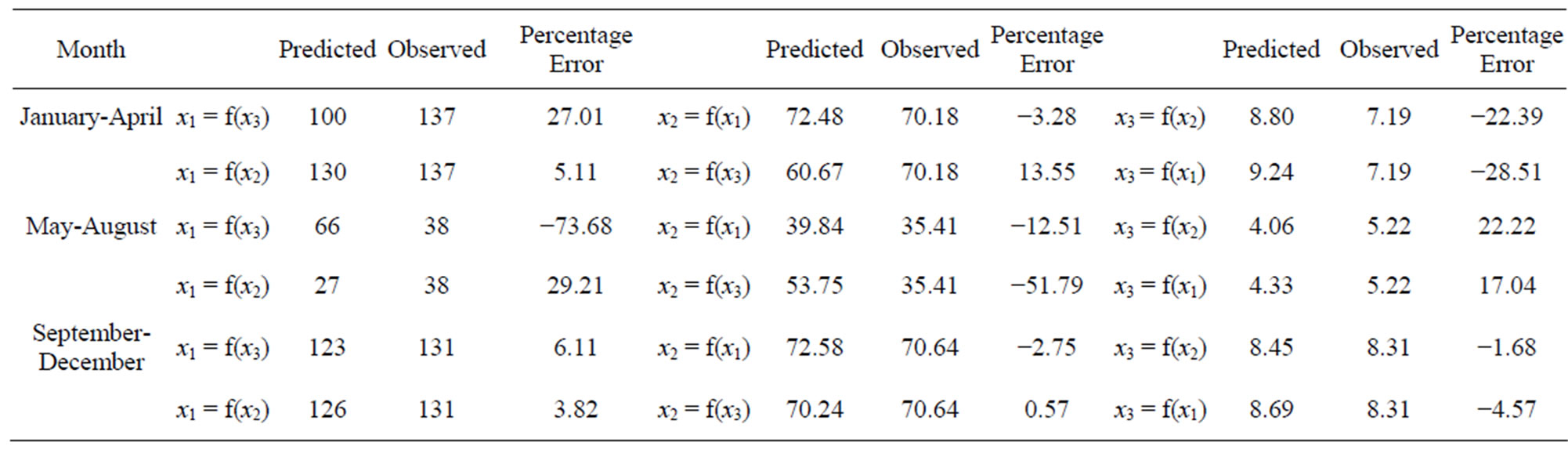
Table 20. Predicted value of x1, x2 and x3 considering every pair of parameters.
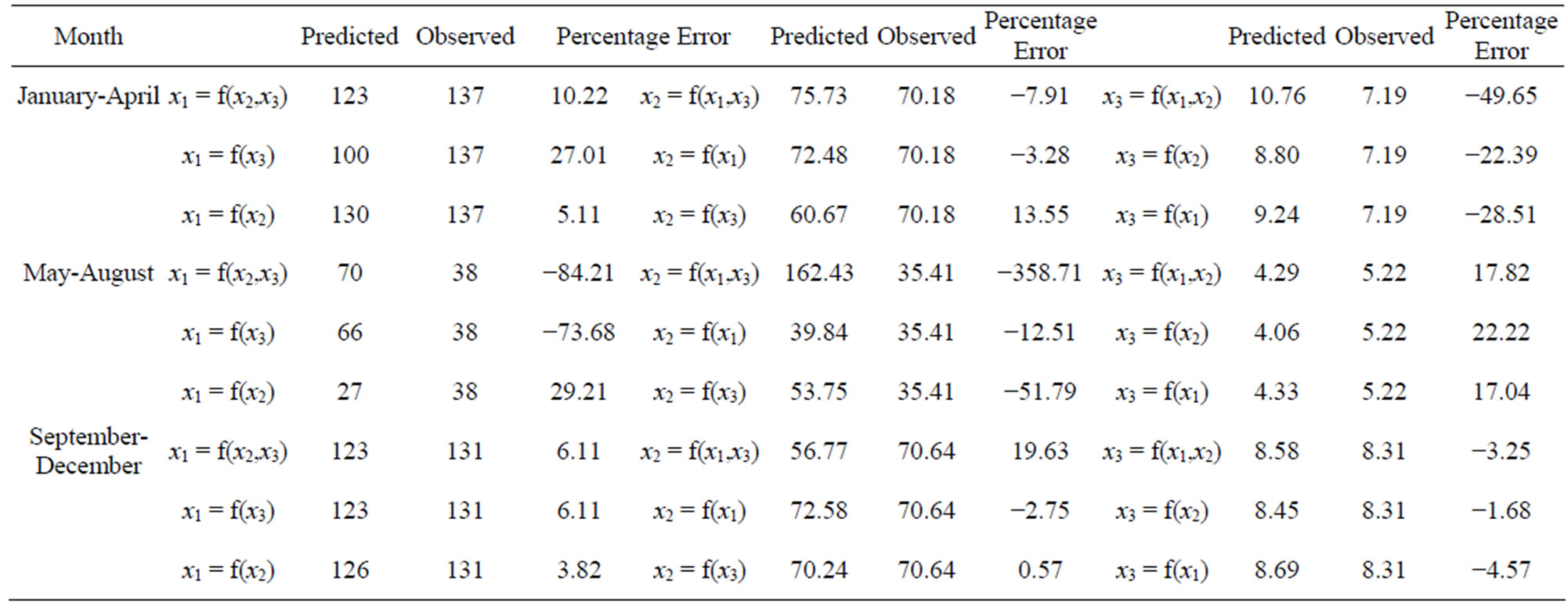
Table 21. Comparative studies of errors for different cases.
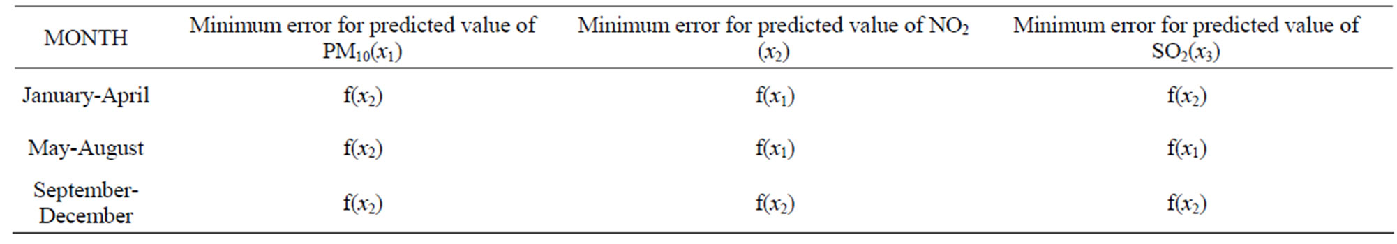
Table 22. Season-wise identification of dependent variable to predict each parameter with minimum error.
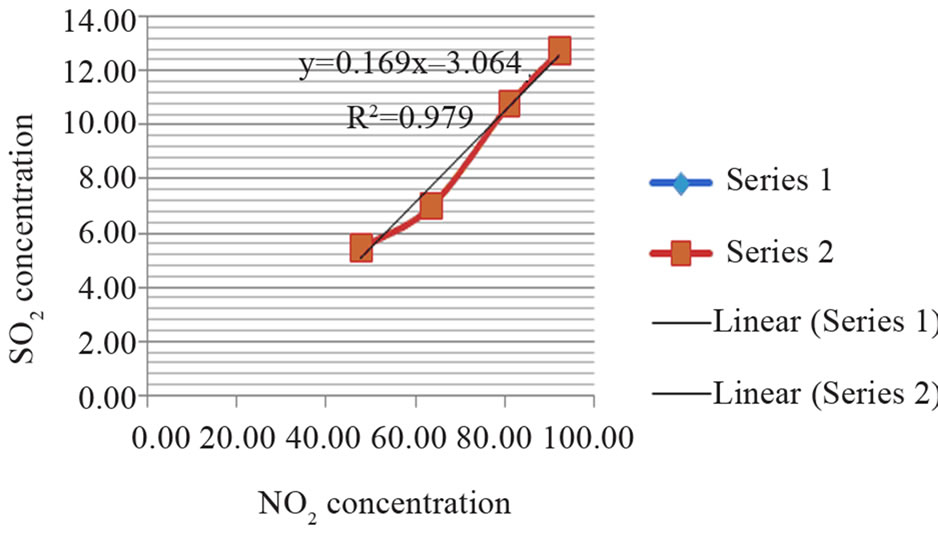
Figure 10. Interrelation between SO2 and NO2.
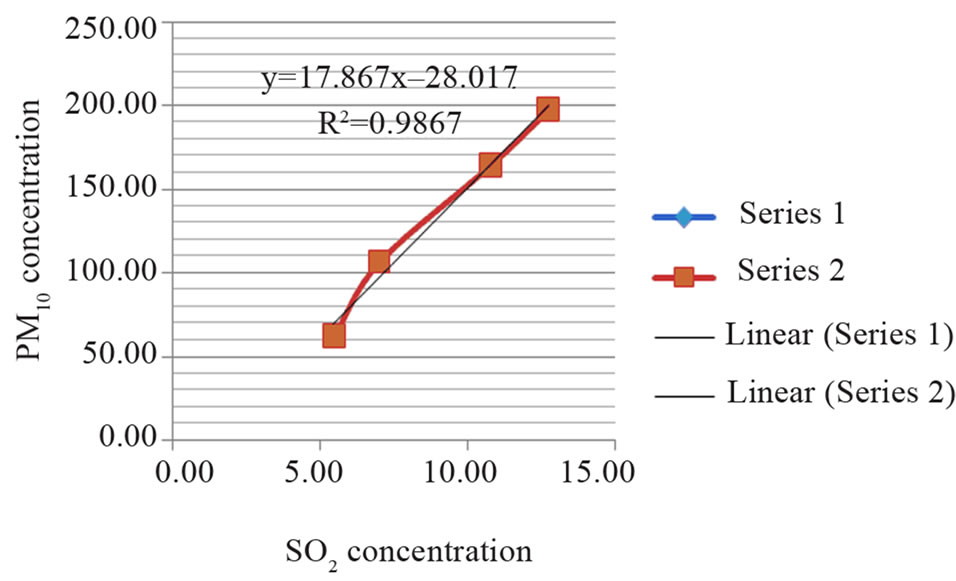
Figure 11. Interrelation between SO2 and PM10.
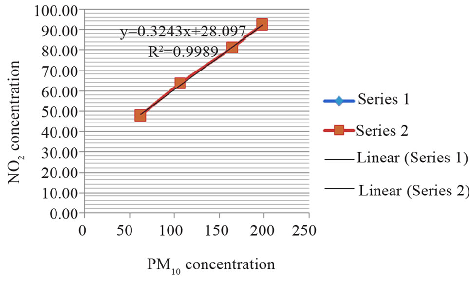
Figure 12. Interrelation between NO2 and PM10.
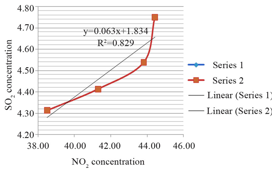
Figure 13. Interrelation between PM10 and SO2.
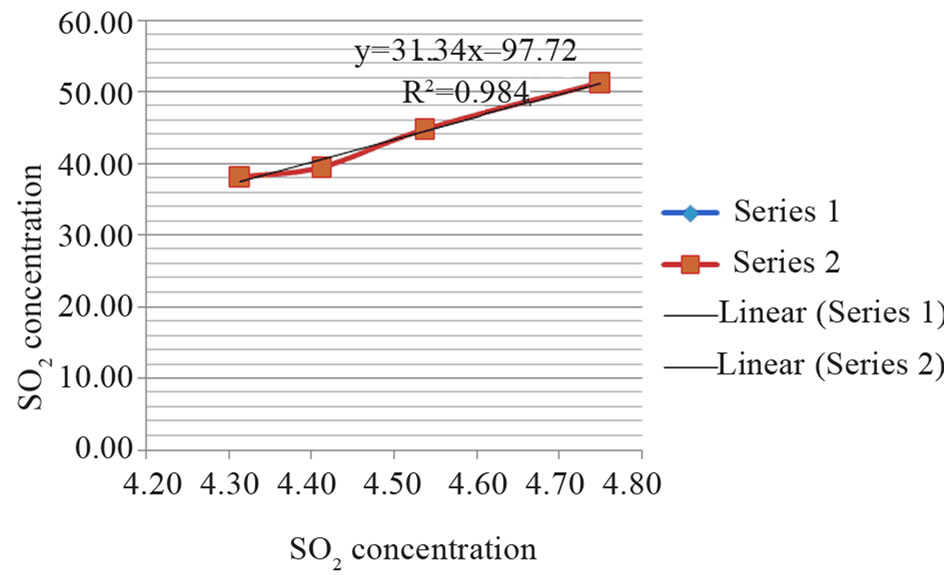
Figure 14. Interrelation between NO2 and PM10.
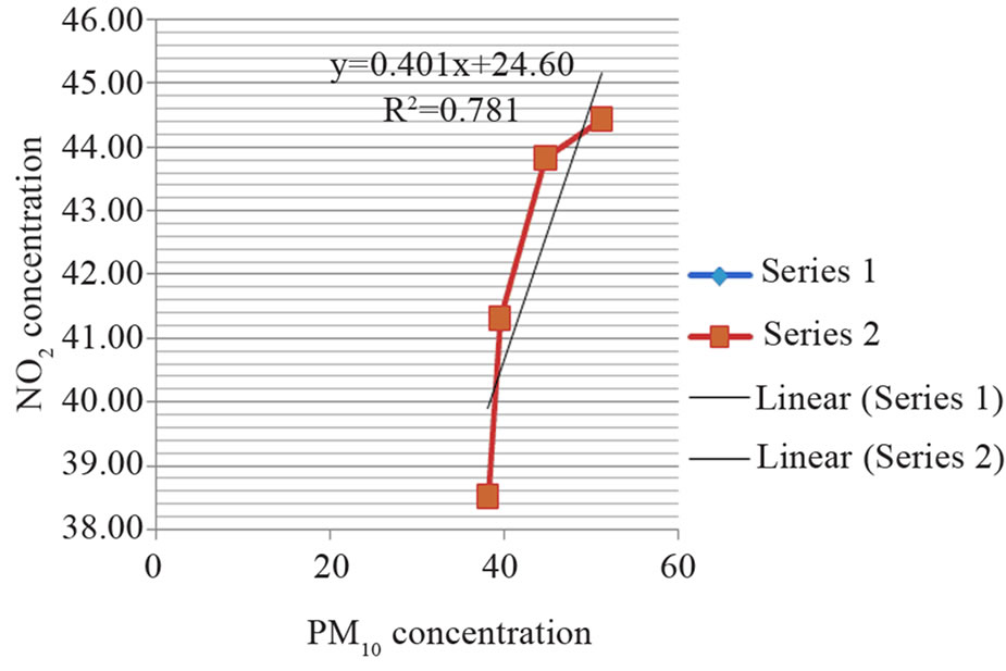
Figure 15. Interrelation between NO2 and SO2.
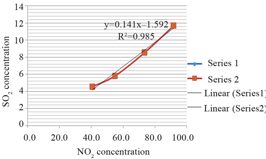
Figure 16. Interrelation between NO2 and SO2.
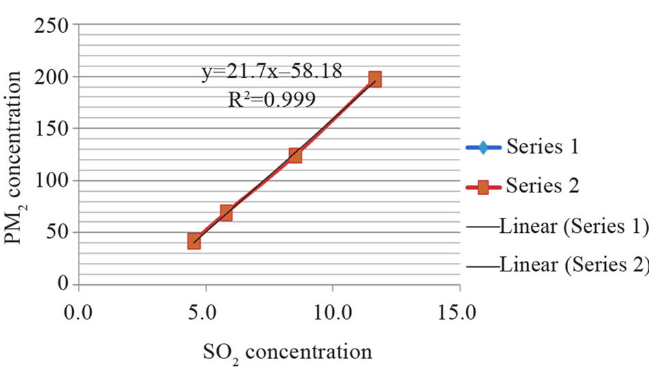
Figure 17. Interrelation between PM10 and SO2.
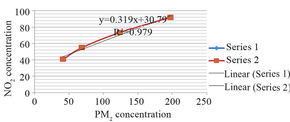
Figure 18. Interrelation between NO2 and PM10.
5. Conclusion
As different parameters are involved for dispersion of pollutants in atmosphere, it is not possible to achieve 100% accuracy for prediction in most of the cases due to different climatic parameters, sampling errors etc. Our study involves the prediction of major three types of pollutants and tries to give an idea about their levels which may help many future activities. If we follow the method given in our paper we find that instead of collecting all types of data, we need to measure only two types of parameters depending on the time periods. For example, prediction of PM10 can be made using the value of any one of the parameters NO2 and SO2. However, it is interesting to observe that prediction of PM10 is more accurate when only the value of NO2 is used instead of SO2. Thus during the process of data collection if sample of NO2 is only collected, our purpose would be served and, consequently, the cost involved in the field work to collect samples can be significantly reduced. As we know SO2, NO2 and PM10 have very negative impact of on our society; their predictions may help us adopt necessary preventive measure time to time to ensure better living conditions.
REFERENCES
- D. Majumdar, A. K. Mukherjee and S. Sen, “BTEX in Ambient Air of a Metropolitan City,” Journal of Enviornmental Protection, Vol. 2, No. 1, 2011, pp. 11-20. doi:10.4236/jep.2011.21002
- A. B. Chelani and S. Devotta, “Non-Linear Analysis and Prediction of Coarse Particulate Matter Concentration in Ambient Air,” Journal of Air and Waste Management Association, Vol. 56, No. 1, 2006, pp. 78-84.
- “Air Quality Status for Ten Cities of India, for 1999 & 2000,” National Environmental Research Institute, Nagpur, 2011.
- Website of National Ambient Air Quality Standard, “Central Pollution Control Board; Ministry of Environment and Forests,” India. http://cpcb.nic.in/National_Ambient_Air_Quality_Standards.php
- M. K. Ghosh, “Air Pollution in the City of Kolkata: Health Effects due to Chronic Exposure,” Environmental Quality Management. doi:10.1002/tqem/Winter
- C. H. Lai and K. S. Chen, “Characteristic of C2-C15 Hydrocarbons in the Air of Urban Kaohsiung,” Atmospheric Environment, Vol. 38, No. 13, 2004, pp. 1997-2011. doi:10.1016/j.atmosenv.2003.11.041.
- X. Wang, S. Guo, J. Fu, C. Chan, S. C. Lee, L. Y. Chan and Z. Wang, “Urban Roadside Aromatic Hydrocarbons in Three Cities of the Pearl River Delta, People’s Repub-lic of China,” Atmospheric Environment, Vol. 36, No. 33, 2002, pp. 5141-5148. doi:10.1016/S1352-2310(02)00640-4
- E. Ilgen, N. Karfich, K. Levsen, J. Angerer, P. Schneider, J. Heinrich, H. E. Wichmann, L. Dunemann and J. Begerow, “Aromatic Hydrocarbons in the Atmospheric Environment: Part I. Indoor Versus Outdoor Sources, the Influence of Traffic,” Atmospheric Environment, Vol. 35, No. 7, 2001, pp. 1235-1252. doi:10.1016/S1352-2310(00)00388-5
- West Bengal Pollution Control Board, “Rising up to the occasion,” Department of Information & Cultural Affairs Government of West Bengal Writers’ Buildings, Kolkata, 2006.
- Website of Daily Ambient Air quality Information of West Bengal. http://emis.wbpcb.gov.in/airquality/citizenreport.do