American Journal of Climate Change
Vol. 2 No. 3A (2013) , Article ID: 37407 , 15 pages DOI:10.4236/ajcc.2013.23A005
Extremes of Severe Storm Environments under a Changing Climate
1Department of Statistics, North Carolina State University, Raleigh, NC, USA
2Research Applications Laboratory, National Center for Atmospheric Research, Boulder, CO, USA
Email: mannshardt@stat.ncsu.edu
Copyright © 2013 Elizabeth Mannshardt, Eric Gilleland. This is an open access article distributed under the Creative Commons Attribution License, which permits unrestricted use, distribution, and reproduction in any medium, provided the original work is properly cited.
Received June 19, 2013; revised July 22, 2013; accepted August 25, 2013
Keywords: Projections of Extreme Events; Reanalysis; Severe Storms; Extreme Weather; Generalized Extreme Value Distribution (GEV); Block Maxima
ABSTRACT
One of the more critical issues in a changing climate is the behavior of extreme weather events, such as severe tornadic storms as seen recently in Moore and El Reno, Oklahoma. It is generally thought that such events would increase under a changing climate. How to evaluate this extreme behavior is a topic currently under much debate and investigation. One approach is to look at the behavior of large scale indicators of severe weather. The use of the generalized extreme value distribution for annual maxima is explored for a combination product of convective available potential energy and wind shear. Results from this initial study show successful modeling and high quantile prediction using extreme value methods. Predicted large scale values are consistent across different extreme value modeling frameworks, and a general increase over time in predicted values is indicated. A case study utilizing this methodology considers the large scale atmospheric indicators for the region of Moore, Oklahoma for Class EF5 tornadoes on May 3, 1999 and more recently on May 20, 2013, and for the class EF5 storm in El Reno, Oklahoma on May 31, 2013.
1. Introduction
One of the more critical issues with a changing climate is the behavior of extreme weather events, as these can cause loss of life, and have huge economic impacts. Currently, the average advance warning time for an approaching tornado is 5 - 13 minutes. Any increase in the advance warning time could be vital for preventing economic loss as well as for saving lives. Atmospheric sounding readings provide a measure of the energy systems in the atmosphere. Convective available potential energy (CAPE) and wind shear (WS) are indicators for ideal storm conditions, and can be predicted in real-time up to three hours before severe storms occur. Changes in these indicators can result in conditions that favor severe storms. Understanding the extreme behavior of these indicators could lead to real-time improvements in the advance warning times for possible severe storms. It is also important to understand whether the magnitude and frequency of these large scale indicators might be increasing over time. Here we consider extreme value analysis models for re-analysis data over the United States to explore the possibility of considering the large scale indicators of severe weather events and their behavior over time.
Numerous studies have been conducted pertaining to the characterization of environments that are conducive to severe thunderstorm activity and tornadic events (e.g., Brooks et al., 2003 [1]; Craven and Brooks, 2004 [2]. Molinari and Vollaro (2010) [3] examine the impact and interactions of atmospheric sounding readings including CAPE and WS on storm intensity. Definitions of storm classifications (Non-severe, Severe, Significant Nontornadic, Significant Tornadic) are provided in [1]. CAPE and WS are found to be associated with atmospheric conditions that exist during the occurrence of thunderstorms and tornadoes. Gilleland et al. (2013) [4] shows the distinction between the cumulative distribution functions by storm classification, and the distinction between the probability density functions of CAPE × Shear and WmSh for the different storm classifications, where WmSh is a function of CAPE and WS. A statistical summary of the distribution for WmSh by storm classification is provided in Table 1. Clearly, as the storm classifica-
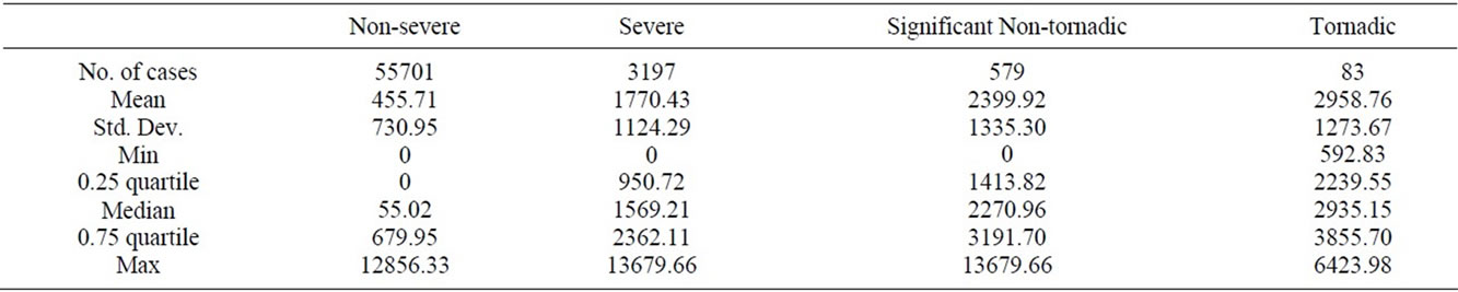
Table 1. Statistical summary of the distribution of WmSh (m2/s2) by storm classification (cf. Brooks, 2004).
tion intensifies, the number of cases decreases (there are fewer extremely severe storms), so caution is necessary in making any inferences about the distributions shown in the figure. Nevertheless, with 83 cases for the most severe category (tornadic), one can be reasonably certain that the distributions shift to higher values for both variables.
Convective available potential energy and wind shear are considered as large scale indicators of severe weather, as over land, high values of both variables together are characteristic of an environment conducive to severe weather. It is the extreme values of the processes that are of interest, which combined with the presence of a possible time trend, introduces new statistical challenges. Trapp et al. (2009) [5] look at frequencies of exceeding a threshold for areal averaged CAPE times WS (conditioned on having CAPE ≥ 100 J/kg and WS ≥ 5 m/s) and Marsh et al. (2007) [6] take the average over space to consider comparisons, but neither explore an extreme value approach for large scale indicators. Gilleland et al. (2008) [7] presents a preliminary investigation fitting an extreme value distribution individually at each location to investigate linear trends in the location parameter, whereas in this work the temporal relationship is more fully explored and showcases a case study. Heaton et al. (2010) [8] examine a spatial-temporal model for large scale indicators with focus on modeling the WmSh process, whereas here we are interested in investigating a possible change in the distribution of extremes of large scale indicators over time.
This paper outlines an extreme value approach for analyzing large scale indicators of severe weather through the consideration of WmSh. Various approaches utilizing extreme value theory for block maxima, including examination of a trend over time, are implemented for reanalysis data over the United States. Section 2 provides a description of the data and Section 3 details a study of the empirical frequency of exceeding large values. Section 4 outlines the methodology of extreme value theory, followed by Section 5 which details the extreme value analysis of WmSh. A case study of the recent tornadoes in Oklahoma is explored in Section 6. Finally, a summary of major findings is presented in Section 7 with a discussion in Section 8.
2. Data
For the present study, CAPE and WS, provided by H.E. Brooks, were calculated from the National Center for Environmental Prediction (NCEP)/National Center for Atmospheric Research (NCAR) reanalysis data (Kalnay et al., 1996) [9]. The dataset used here covers 42 years (1958-1999) of four times daily sounding readings over 884 sites covering North America at a resolution of approximately 1.875˚ longitude and 1.915˚ latitude. The maximum of the four values of each variable per day is taken to produce a daily observation, and to remove some temporal dependence. For the product variables, the product is taken before the maximum to ensure that the maximum product for each day is taken. Statistically, the data are very non-Gaussian and characterized by many zero or near-zero values. Depending on the region, some grid points never reach very high values, where others (e.g., over the central United States) are relatively very large relatively often.
Define WmSh = Wmax × WS, where wind shear (WS) is measured in meters/second, Wmax =![]() , and CAPE = Convective Available Potential Energy, measured in Joules/kg. Using Wmax rather than directly modeling CAPE has the advantage that Wmax and WS are in the same units.
, and CAPE = Convective Available Potential Energy, measured in Joules/kg. Using Wmax rather than directly modeling CAPE has the advantage that Wmax and WS are in the same units.
3. Empirical Frequency of Exceeding Large Values
As an initial exploratory analysis of whether these frequencies have been changing over the 42-year period, Figure 1 shows the probabilities of WmSh’s exceeding 1000 m2/s2 for each of three time periods: 1958-1969 (top left), 1970-1984 (top right), and 1985-1999 (lower left). This threshold is chosen because it represents relatively lower quantiles of the distributions of WmSh for the more severe storm types, versus a rather high quantile for the non-severe storm type (cf. [1]). From these plots, it is difficult to see any discernible difference from one period to the other. The plot in the lower right shows the ratio of the most recent period (1985-1999) to those of the earliest period (1958-1969) with 0.01 added to both numerator and denominator in order to avoid division by

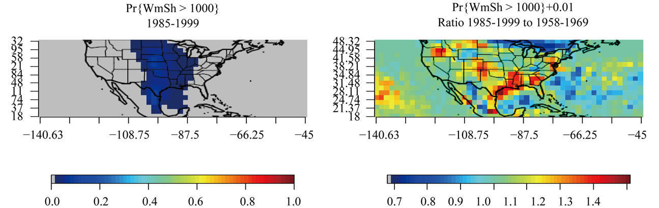
Figure 1. Point-wise probabilities of WmSh’s exceeding 1000 m2/s2 for 1958-1969 (top left), 1970-1984 (top right), and 1985- 1999 (lower left). Ratio of probabilities for 1984-1999 (+0.01) to those for 1958-1969 (+0.01). Left color scale applies for first three plots, right color scale only for lower right plot.
zero, and maintain comparability. Clearly, much of the region has not changed appreciably with respect to the frequency of exceeding 1000 m2/s2. All of the values are close to unity, indicating that the frequency of WmSh values exceeding 1000 m2/s2 has not changed. However, the Gulf Coast states appear to have a potentially higher frequency of this event’s occurring. The ratio of probabilities, shown in the bottom right plot of Figure 1, shows increasing trends over the Gulf Coast and central North America, with decreases seen over the region including Great Lakes and South Eastern Canada.
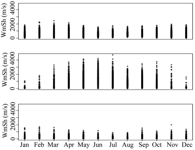
Figure 2 shows the daily WmSh (m2/s2) time series across the entire 42-year period for three individual grid points in the vicinities of Havana, Cuba (top), northwestern Oklahoma, USA (middle) and southern California, USA (bottom). Clearly, the values tend to have higher magnitude over northwestern Oklahoma than the other two locations, and Cuba tends to have moderately higher values than southern California. There do not appear to be any long term trends in any of these series, which is consistent with the above exploratory analysis. There is perhaps a periodic structure in them, but it is difficult to discern over the entire time length. Figure 3 shows the same series as Figure 2, but for only the year 1958. From this figure, it can be seen that the intra-annual behavior of WmSh varies wildly for each site. Cuba has moderately high, but relatively constant values throughout the year, Oklahoma has very low values in the winter, and extremely high values in the summer months, and southern California shows relatively low values for the entire year.
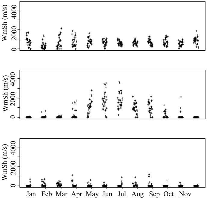
Finally, Figure 4 shows the entire 42-year series for these same three grid points by month. It can be seen from this figure that the behavior of WmSh is relatively constant from year to year for Cuba and southern California, but the sharp peaks for northwestern Oklahoma stretch over more of the year than they did for 1958 alone. In looking at the long-term behavior of frequencies of higher values of WmSh, it would seem prudent to account for the annual variability. While it might be reasonable to exclude November through February for northwestern Oklahoma, it is not clear that this strategy would work well for arbitrary grid points. Therefore, careful study of each region is necessary before applying a model for the frequencies.
4. Methodology: Extreme Value Theory
When dealing with extreme events, the values of interest lie in the tail of the distribution of the corresponding process. Even if the underlying distribution is known, estimation error for the corresponding parameters will be compounded in the high percentiles of the tails. Thus it is necessary to develop methodology to model the tail of the distribution directly. Extreme value theory offers a well-defined framework for the asymptotic properties of the tails of probability distributions.
4.1. Annual Maxima Approach
Consider the natural blocks of interest for the series under which the observations are measured, e.g. daily, yearly,
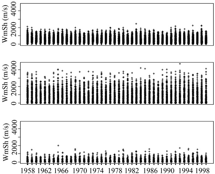
Figure 2. Daily WmSh (m2/s2) values from 1958-1999 for three grid points: around Havana, Cuba (top), northwestern Oklahoma, USA (middle) and southern California, USA (bottom).
etc. In many environmental applications, temporal observations are measured hourly or daily, where the year is the natural block of interest for the series. Under certain normalizing conditions (see Coles, 2001 [10]), the block maxima of the series can be modeled using a limiting form of an exponential distribution, known as the Generalized Extreme Value (GEV) distribution.
Let X represent the annual maximum of daily observations in a given series. The Generalized Extreme Value (GEV) distribution is defined by the formula
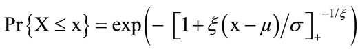 (1)
(1)
where y+ = max{y, 0}, µ is a location parameter, σ a
scale parameter and ξ is the extreme-value shape parameter; µ and ξ can take any value in (−∞, ∞), but σ must be positive. The notation (• • •)+ follows the convention x+ = max(x, 0) and is intended to signify that the range of the distribution is defined by . In other words,
  when ξ > 0,
  when ξ > 0 (cf. [10]; Smith, 1990 [11]).
4.2. Parameter Interpretation: Return Levels
It is difficult to directly interpret the parameter estimates, but it is convenient to investigate the associated return levels, which are a function of the parameters from the Generalized Extreme Value distribution. The n-year return level, rn, is the level so extreme it is expected to occur once every n years. Note that the n-year return level corresponds to the (1 – 1/n) quantile of the predictive distribution. An advantage of using the block maxima approach is the estimated parameters are directly interpretable in terms of the return levels.
The n-year return value is formally defined by setting Equation (1) to 1 – 1/n; rn is then the solution to the resulting equation. In practice, however, for large n we have 1 − 1/n ≈ e−1/n and it is more convenient to define rn by the equation:
which leads to the formula
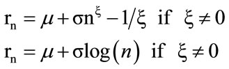 (2)
(2)
4.3. Tail Behavior
The shape parameter ξ is also of interest. The shape parameter determines the tail behavior of the extreme value distribution. A shape parameter value of ξ = 0 indicates a flat tail and corresponds to a limiting distribution of the Gumbel exponential form. Values between −0.5 and 0.5 are commonly seen, with negative values indicating a bounded tail [12] and positive values indicating unbounded, heavier tails.
4.4. Temporal Trend Model
In order to consider whether the extreme behavior is changing over time, a model incorporating a time component can be investigated. For a temporal model, the time component is considered by including a trend in the parameters of the generalized extreme value distribution.
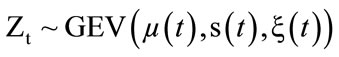
Define Zt, the annual WmSh level as:
 (3)
(3)
where for trend of interest ∑kµk∗fk(t) for 0 ≤ k ≤ u, with fk(t) a function of time such as a quadratic or linear trend, k the number of terms in the function of time, µk the kth term’s coefficient, and t representing the year.
As explored in Katz et al. 2005 [13] and Mannshardt et al. 2013 [14], a shift in the location parameter of an extreme value distribution can indicate a shift in the overall distribution.
Under the temporal trend model, the return values are:
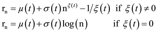 (4)
(4)
It is important to make the distinction between the timeframe defined by the return period and t. For the n-year return level, n is the timeframe defined by the return period. n = 10, 20, 50, 100 are return periods often considered in environmental applications. The temporal trend time period is defined by t, where t is the time at which the n-year return level is being calculated. Prediction utilizing the temporal trend coefficients significantly beyond the time period for which the model was fit could lead to misleading results due to extrapolation. Therefore for the temporal trend models we restrict our attention to values of t = 1, ..., 60. We consider the 20 years return levels from the temporal trend model as well as the no trend model in order to enable a comparison of the trend over time t for return levels within the time period used for model estimation. This also enables empirical validation with the 0.95 quantile of WmSh. It would be valid inference to consider the 50 or 100 years return levels for the models used here, where 50 or 100 would be the timeframe defined by the return period, though for the purposes of this paper we restrict our attention the 20 years return levels.
5. Extreme Value Analysis Results
We are interested in predicting the 20 years return levels of WmSh for the region of interest over North America including the continental United States. Recall that the n-year return level, rn, is the level so extreme it is expected to occur once on average every n years, and for the GEV fit to annual maxima of the data, corresponds to the (1 – 1/n) quantile. Thus the 20 years return level for WmSh corresponds to the 0.95 quantile of the distribution of WmSh. We consider a comparison of a GEV model under the assumption of no trend over time to models incorporating a temporal trend through different parameterizations. The generalized extreme value distribution for block maxima is fit to the time series at each of the 884 sites. The block maxima model is chosen for this analysis over alternative models such as a Peaks Over Threshold approach (cf. [10]). The main reason is for the interpretability of the location parameter of the GEV distribution, as a possible shift in distribution over time is ultimately of interest and is considered using a model with a temporal trend in the location parameter. Spatial patterns are evaluated, however no spatial trend is incurporated. The significance of the various time trend models is evaluated, and the 20 years return levels are calculated under each modeling framework. Analysis is done using the R (R Development Core Team, 2009 [15]) packages extRemes (Gilleland et al., 2009 [16]) and ismev (cf. [10]).
5.1. Annual Maxima Analysis for WmSh
Figure 5 shows the 20 years return levels for WmSh as calculated using Equation (2), corresponding to the 0.95 quantile of the distribution of WmSh. The top left shows the 20 years return levels resulting from fitting the GEV model; the empirical distribution for WmSh is shown in the top right. The lower and upper 95% confidence bounds are also shown (bottom) for the fitted return levels. The modeled 20 years return levels of WmSh are consistent with the empirical 20 years return levels, i.e. the empirical 0.95 quantiles. This helps to validate the use of the Generalized Extreme Value distribution for modeling the return levels of WmSh.
5.2. Tail Behavior: The Shape Parameter
For the annual maxima approach, ξ is small but positive for most of the stations, which can be seen in the top left plot of Figure 6. If the shape parameter is in fact zero, it suggests that directly modeling the return levels through fitting a Gumbel model may lead to a better fit. To determine whether the shape parameter is significantly different from zero, 80% confidence intervals for ξ are constructed to test the null hypothesis that ξ = 0 versus the alternative hypothesis that ξ is not zero. Figure 6 shows the estimates of ξ (top left), with the corresponding 80% confidence intervals (bottom). Note that the confidence intervals are not adjusted for multiple com-
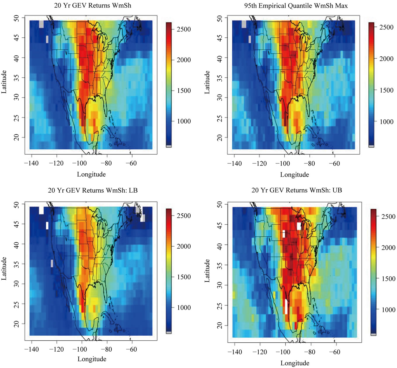
Figure 5. Generalized extreme value analysis, including the 20 years return levels (top left), 95% quantile (top right), and 95% lower and upper confidence bounds (bottom) for the estimated return levels.
parisons orspatial correlation. The top right plot in Figure 6 indicates the locations where ξ is significantly different from zero; non-significance is indicated in green, significantly less than zero in blue and significantly greater than zero in red.
Generally, this indicates a light and bounded upper tail behavior, which is consistent with the physics of WmSh in that there are physical properties constraining them from being very high simultaneously. At some locations, the shape parameter may not be significantly different from zero, but a three parameter model may still be the correct model. One consideration is the standard errors. The standard error estimates for the shape parameter may be too conservative, for which there are several considerations beyond the scope of this paper but are worth investigation for future applications. Here we are fitting the model to a limited number of data points, by utilizing only the annual maxima (nmax = 42). Additional methods, including a Peaks Over Threshold approach (cf. [10]), or methods taking advantage of spatial dependence (Cooley and Sain, 2011 [17]), could be considered.
We retain the use of the 3-parameter model as it was signficant for 350 of the 884 locations, and is ultimately more flexible. Additionally, while not detailed here, a Peaks Over Threshold model was fit to examine the tail behavior under a model incorporating more data points and the results support a non-Gumbel model.
5.3. Temporal Analysis
It is clear from Figure 1 that the empirical distribution of WmSh is changing over time. Thus it is of interest to
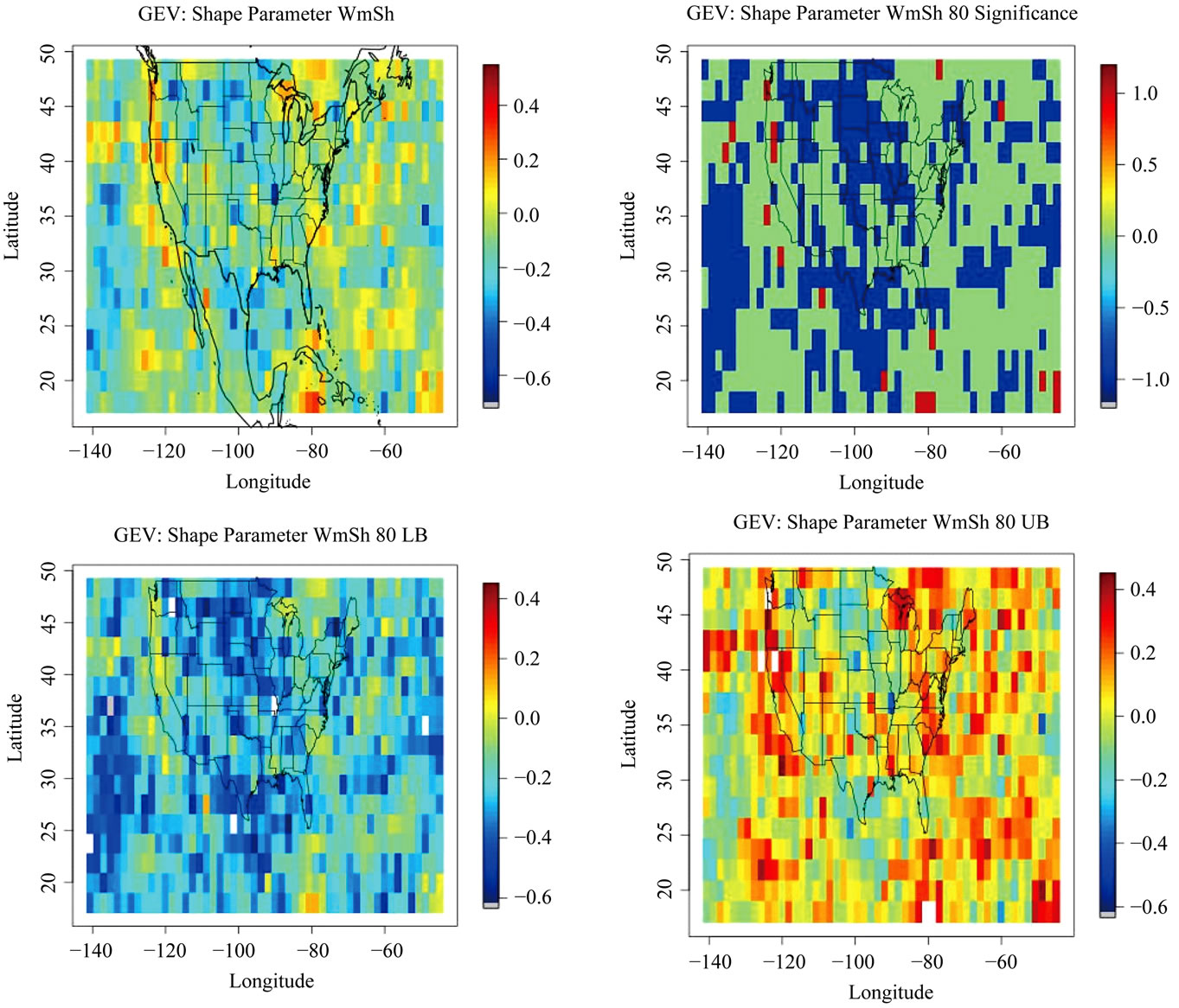
Figure 6. Shape parameter ξ (top left), its significance (top right) and the 80% lower and upper confidence bounds (bottom).
examine a temporal trend model. We consider a linear temporal trend model as well as a quadratic model in time for the location parameter of the generalized extreme value distribution of large scale indicator WmSh, and examine the behavior and predictive properties.
5.4. Linear Temporal Trend Model
For a simple linear trend temporal model, the time component is considered through a linear trend in the location parameter µ. Therefore Z, the annual WmSh level, is Zt ~  where µ(t) = µ0 + µ1t* with t* representing the standardized year for t = 1, ..., 42 for t corresponding to the 42 years in the reanalysis series of WmSh.
The top left plot of Figure 7 shows that the return values for the linear time trend model are consistent with the non-temporal GEV analysis. The top left shows the 20 years return levels estimated at the 40th year, where t = 40 is the 20-year return value seen at year 40 of the time series, which is comparable to the original 20-year return values resulting from the GEV model fit with no time trend for the 42 years in the original series of annual maxima. The interpretation of the location parameter can be seen in Figure 7. The top right shows the return values for the linear time trend versus the return values for no trend. The plot indicates relative agreement between the return values, suggesting that the linear trend model is a good fit. The bottom left plot of Figure 7 shows that there is a positive trend in the time coefficient for the location parameter of the generalized extreme value distribution across most of the continental US, particularly over the Mid-West region. The bottom right shows the significance at the 80% level of the linear time trend coefficient against a null hypothesis of no significance; coefficient estimates which are significantly greater than zero are shown in red, significantly less in blue, and non-significance in green.
To consider the possible change in trend for the loca-
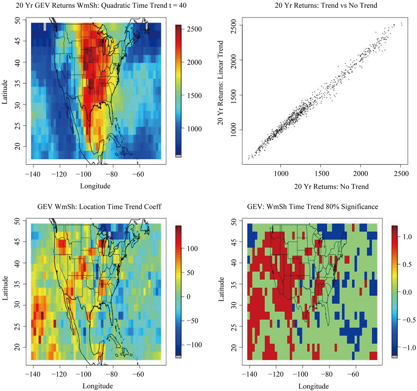
Figure 7. Temporal analysis: 20 years return levels for the linear trend model in time for WmSh (top left); comparison of return values for the Linear Trend model to No-Trend model (top right); location parameter time coefficient for WmSh (bottom left) and the significance of the linear time coefficient (bottom right).
tion parameter of the extreme value distribution of WmSh over time, the 20-year return values are calculated at different points in time, for t = 40, 60, 100, where t is the standardized t* values used in the model fitting. Figure 8 shows that there is an increasing trend in the return values over time across most of the continental US, particularly over the Mid-West region. This indicates that the location of the extreme value distribution for WmSh is shifting towards higher values over time. Again, t = 40 is the 20-year return value seen at year 40 of the time series, which is comparable to the original 20 years return values resulting from the GEV model fit with no time trend. (Note that in order to show differentiation across the different values of t, here the color scale is different than in previous figures. The 20 years return levels for t = 40 shown in the middle plot of Figure 8 are identical to the values in the top left plot of Figure 7, and are simply shown on a different color scale in order to consider regional patterns). Thus a positive linear time trend coefficient suggests that WmSh is increasing over the time period examined.
5.5. Tail Behavior in Linear Time Trend
The shape parameter ξ (tail parameter) is also of interest for the temporal trend, as the shape parameter determines the boundedness of the extreme value distribution. A fully temporally parameterized model was fit where
in order to investigate any possible trend in the tail pa-
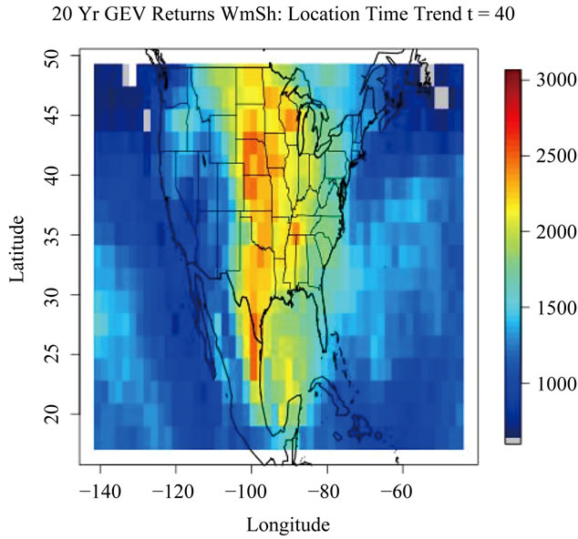
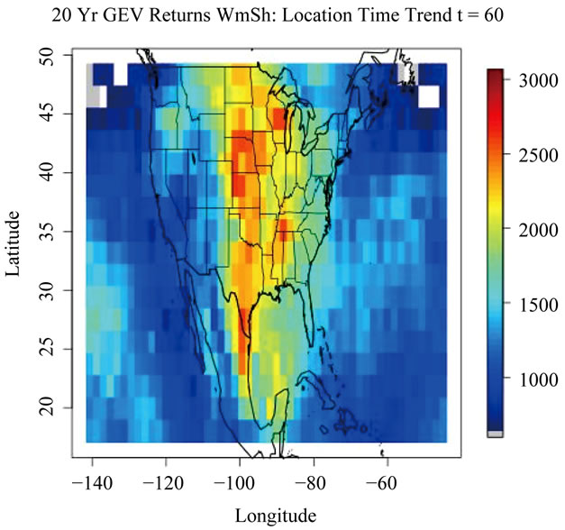
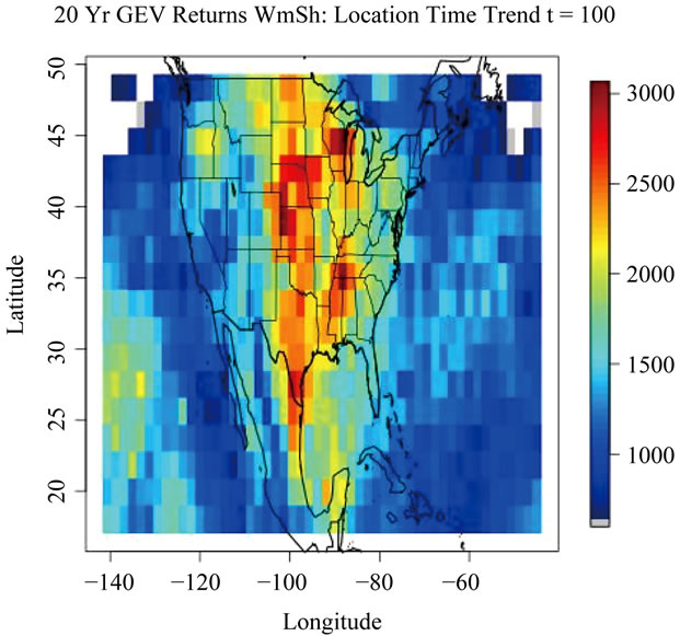
Figure 8. GEV 20-yr return values for WmSh with a time trend in the location parameter. Shown for t = 40, 60, and 100. Note that in order to show differentiation across the possible values of t, the color scale is different than in previous figures.
rameter over time.
The top left plot in Figure 9 shows the estimates of the intercept for ξ in the linear time trend model, with the corresponding standard errors (top right). The bottom left plot in Figure 9 shows the estimates of the coefficient or the linear time trend in ξ with the corresponding standard errors (bottom right). The tail behavior for the linear time trend model overall shows similar behavior as seen in Figure 6 for the no-trend model. There is little evidence of the tail behavior changing over time, as the estimates for the linear temporal trend coefficient are close to zero.
5.6. Quadratic Trend in Time
In order to allow for a more flexible trend in time, a quadratic temporal model is also considered with the time component a quadratic trend in the location parameter µ. Therefore Zt, the annual WmSh level, is Zt ~  where µ(t) = µ0 + µ1t* + µ2t**, where t* and t** are the standardized values of t and t2 respectively. The scale and shape parameter are taken to be constant over time.
The top plots of Figure 10 shows that the return values for the quadratic time trend model are consistent with the non-temporal GEV analysis. The top left shows the 20 years return levels estimated at the 40th year, which is comparable to the original 20 years return values resulting from the GEV model fit with no time trend.
The interpretation of the trend in the location parameter can be seen in Figure 10, where the top right shows the return values for the quadratic time trend versus the return values for the linear time trend. The plot indicates relative agreement between the return values, however does show a little dispersion around the higher return levels, indicating that the models differ slightly in how the time trend affects the return levels estimated for each model. To consider the possible change in trend for the location parameter of the extreme value distribution of WmSh over time, the 20-year return values are calculated at different points in time, for t = 40, 60, 100, where t and t2 are the standardized t* and t** values used in the model fitting. The middle left plot of Figure 10 shows that there is neutral trend in the linear time coefficient across most of the continental US, however the plot of the quadratic coefficient (bottom left) indicates a positive quadratic effect over most of the continental US. The middle right shows the significance of the linear time trend coefficient at the 80% level and the bottom right shows the significance of the quadratic coefficient; coefficient estimates which are significantly greater than zero are shown in red with significantly less than zero in blue and non-significance in green. In a quadratic model, t2 is the dominating term for the temporal behavior in the location parameter, which if positive indicates an increase in the location parameter over time. A positive quadratic
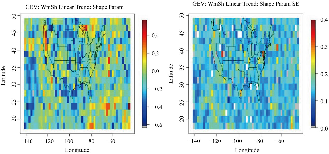

Figure 9. Shape parameter linear time trend coefficient for ξ (left) and the corresponding standard errors (right).
temporal coefficient suggests that the expected magnitude of the WmSh 20 years return levels is increasing over the time period examined. This positive trend is seen over much of the continental United States, with a few areas over the Pacific showing a negative trend.
The return values for the quadratic trend model seen in Figure 11 show that there is an increasing trend in for t = 20, 40, 60 across time across most of the continental US, particularly over the Mid-West region. It can be seen that the return values are increasing in comparison to the return levels seen in the no-trend model and the linear trend model. (Note that in order to show differentiation across the different values of t, the color scale is different than in previous figures). The 20 years return levels (for t = 40) shown in the middle plot of Figure 11 are identical to the values in the top left plot of Figure 10, simply shown on a different color scale in order to consider regional patterns. The increasing estimated return levels for different values of t suggest that the level of extremes expected on average over a 20-year period is increasing over time.
6. Case Study: Moore and El Reno, Oklahoma
We consider a case study utilizing this methodology to evaluate the large scale atmospheric indicators for the region of Moore, Oklahoma for May 3, 1999 and May 20, 2013, as well as El Reno, Oklahoma for May 31, 2013.
Figure 12 shows WmSh for Moore, Oklahoma on May 3, 1999. For 2013, values of CAPE and WS were estimated from the National Oceanic and Atmospheric Ad-

Figure 10. 20 years return levels for the linear trend model in time for WmSh (top left); comparison of return values for the Linear Trend model to No-Trend model (top right); linear time coefficient for WmSh (middle left) and the significance of the linear time coefficient in the quadratic model (middle right); Quadratic time coefficient for WmSh (bottom left) and the significance of the quadratic time coefficient in the quadratic model (bottom right).
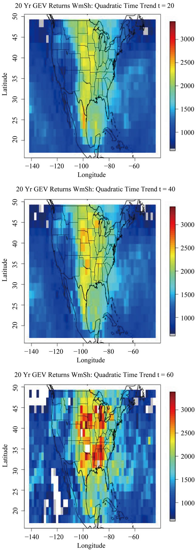
Figure 11. Univariate GEV 20-yr return values for WmSh with a quadratic time trend in the location parameter. Shown for t = 20, 40, and 60.
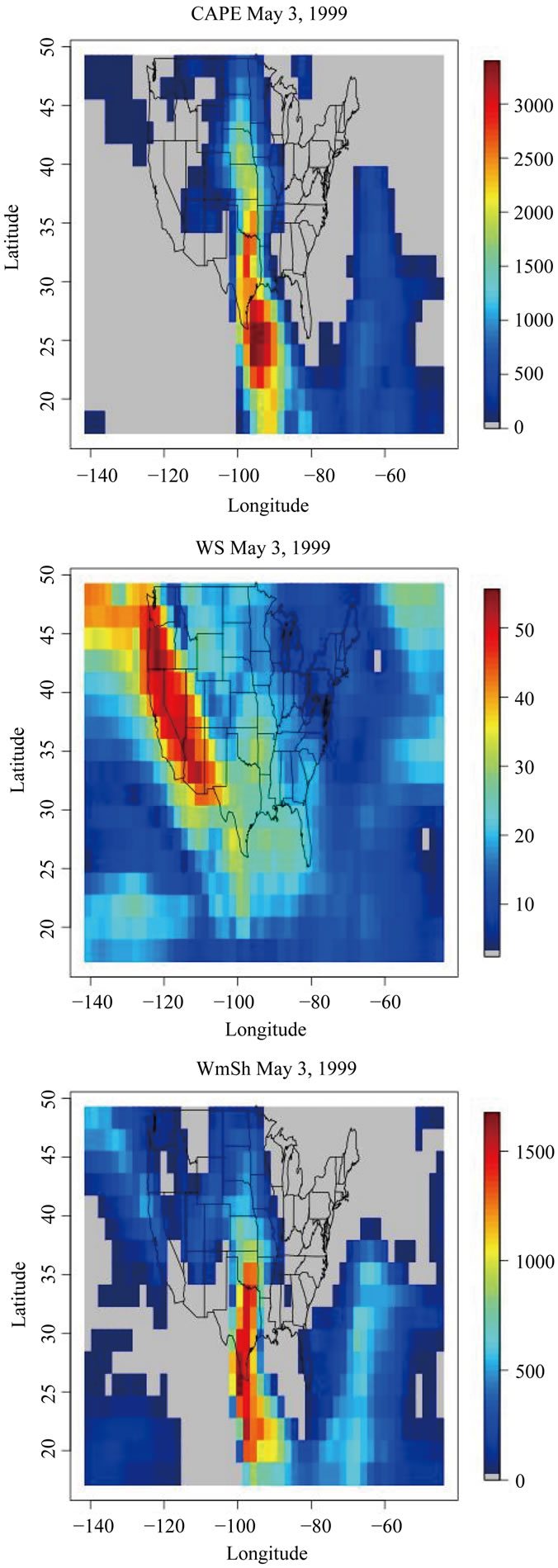
Figure 12. CAPE, WS, and WmSh values on May 3, 1999.
ministration’s (NOAA) Storm Prediction Center (SPC) Hourly Mesoscale Analysis graphical output for atmospheric sounding readings
(http://www.spc.noaa.gov/exper/ma_archive/images_s4). For the time trend models, t is the year in the series used for model fitting. t = 1 corresponds to 1958, and thus 1999 corresponds to the last year in the series used for model fitting, t = 42 and t = 56 corresponds to 2013. The standardized values, t* are used for t to calculate the return period, as in the model fitting and calculation of the 20 years return levels in Section 5.
Table 2 shows the estimated return periods for the values of WmSh observed during each of the tornadic events under each of the three models considered: No time trend, Linear time trend and Quadratic time trend. For the 1999 Moore, Oklahoma tornadic storm, the estimated return period for the observed WmSh = 1654 was n = 1.3. This indicates a value of WmSh is expected to be seen about once every 1.3 years. Note that WmSh = 1654 was well within the range of values observed over the 42 years period (0 - 2475). The location parameter for the no trend model was µ = 1747, which is higher than the observed value of 1654, so this return period validates well with the empirical distribution of WmSh in Moore, OK. The linear and the quadratic time trend models show decreasing return periods respectively, indicating that the severity of this event is becoming less extreme over time; i.e. what was considered a 1.3 years event is a 1.1 years event under the quadratic model, which allows for the changing trend in time.
For the 2013 Moore, Oklahoma tornadic storm, the estimated return period for the observed WmSh = 5020 is n = 402. This is a somewhat large return period, however note that WmSh = 4183 is almost twice that of the largest observed WmSh (2475) over the 42 years period. The linear and the quadratic time trend models show decreasing return periods respectively, indicating that the severity of this event is becoming less extreme over time, with the quadratic model estimating the return period at less than a quarter of the return period under the no trend model.
For the 2013 El Reno, Oklahoma tornadic storm, the estimated return period for the observed WmSh = 5692 is n = 900. Again note that WmSh = 4743 is twice that of the largest observed WmSh (2475) over the original 42 years period with which the model was fit. The linear and the quadratic time trend models show decreasing return periods respectively, indicating that the severity of this event is becoming less extreme over time, with the quadratic model estimating the return period at less than one third of the return period under the no-trend model.
For both the events that took place in Oklahoma in 2013, the temporal trend models show a significant difference in the estimated return periods. The flexibility in incorporating a trend in time allows us to see the changing distribution of extreme values of WmSh as a large scale indicator of extreme tornadic events. What the no trend model would estimate to be a level achieved at the magnitude of several hundreds of years, the quadratic model captures on a much more immediate time frame, with the 2013 Moore event being estimated at a less than 100 years event.
7. Summary
Results indicate that extreme value methods are successful for modeling large scale severe storm indicators CAPE and wind shear as WmSh. Standard extreme value modeling techniques are appropriate for modeling the behavior of WmSh, however there are a few points to consider. For most locations, the shape parameter is not significantly different from zero for the block maxima model. This indicates a light and bounded upper tail behavior, which is consistent with the physics of WmSh. The 3-parameter model is retained for its flexibility in allowing different tail behavior across locations.
Incorporation of a temporal component was successful and showed interesting trends over time. Investigation of the temporal magnitude of changes in WmSh shows slight changes in the location parameter of the extreme value distribution over time, including increasing trends in WmSh over the Gulf Coast and central North America, with decreases seen over the region including Great Lakes. A positive trend in the location parameter over time was seen across the US and especially over the MidWest, for both the linear and the quadratic model in time. This effect is also shown in the 20 years return values for WmSh, which are shown to be increasing across time.
The case study of the tornadic events in Oklahoma showcases an interesting retrospective analysis, as past data was used to evaluate return periods that can be evaluated using current events. The models allowing for
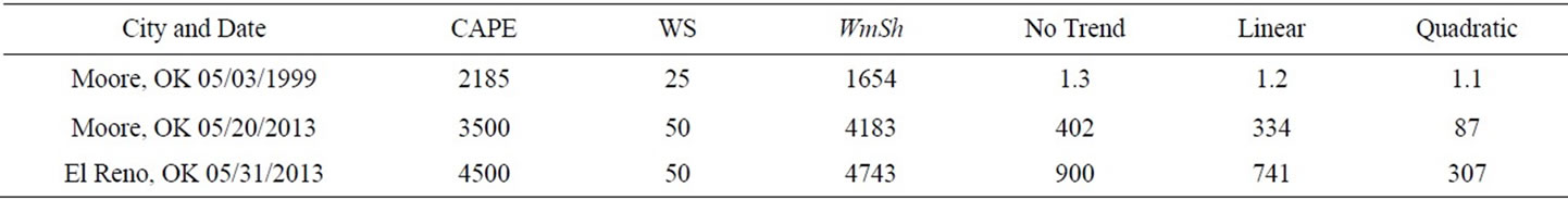
Table 2. Estimated return periods for the values of WmSh observed during each of the tornadic events for the three models considered: No time trend, linear time trend, and quadratic time trend.
a time trend show decreasing return periods, indicating that the severity of these events are becoming less extreme over time. This is an important indication of a positive shift in the distribution of atmospheric sounding extremes, high values of which are conducive to severe thunderstorm activity and tornadic events.
8. Discussion
Results indicate that the generalized extreme value distribution provides a good methodology for modeling the extremes for large scale indicators. A known weakness of the generalized extreme value distribution for block maxima is the tendency to discard data that might in actuality be considered extreme. While beyond the scope of this paper, for similar problems a threshold approach could be utilized—with careful attention given to declustering techniques to account for the fact that extreme weather patterns tend to occur in clusters over time. In addition, while they provide an improvement in data retention, because of the tendency of extremes to occur in clusters and hence violate independence assumptions, threshold methods are susceptible to the same loss of data issues that they are intended to resolve over the block-maxima approaches used in extreme value theory. The standard bias-variance trade-off is considered by Fawcett and Walshaw (2007) [18], who provide an alternative approach to the standard errors which makes use of all of the data above the threshold while addressing the temporal dependence within extreme clusters.
Results suggest spatial dependence as well as multivariate dependence among the different large scale indicators. Spatial extreme is an expanding field, and dependence structures can be introduced in different capacities to address both of these issues. There are several methods that can be investigated to resolve this dependence. Heaton et al. (2010) [8] considered a Bayesian modeling approach to address the tail behavior in physical regions for the indicators across the continental US, which could partially resolve the tail behavior issues occurring in the preliminary results for the global data. These approaches could both be considered.
There is much that can be learned from this initial exploration of the extreme behavior of large scale indicators for severe storm events. Predicting extreme weather events is an important, growing area of research and there remain many avenues for further exploration. The practical applications of properly describing this behavior are vital, given the possible effect of increasing the warning times for severe storms, which ultimately could have a huge human and economic impact.
9. Acknowledgements
The authors thank Harold E. Brooks, Patrick Marsh, Gregory Carbin, and Matt Pocernich for obtaining and providing the data, and supplying initial guidance on this project. This material was based upon work supported by the National Science Foundation (NSF) under Agreement No. DMS-0635449, as well as through the Weather and Climate Impacts Assessment Science Program at the National Center for Atmospheric Research, which is also supported by the NSF. Any opinions, findings, and conclusions or recommendations expressed in this material are those of the author(s) and do not necessarily reflect the views of the NSF. Elizabeth Mannshardt was supported as a Post Doctoral Research Scholar through the National Science Foundation’s Collaborative Research: RNMS Statistical Methods for Atmospheric and Oceanic Sciences under Grant No. DMS-1107046.
REFERENCES
- H. E. Brooks, J. W. Lee and J. P. Craven, “The Spatial Distribution of Severe Thunderstorm and Tornado Environments from Global Reanalysis Data,” Atmospheric Research, Vol. 67-68, 2003, pp. 73-94. http://dx.doi.org/10.1016/S0169-8095(03)00045-0
- J. P. Craven and H. E. Brooks, “Baseline Climatology of Sounding Derived Parameters Associated with Deep, Moist Convection,” National Weather Digest, Vol. 28, 2004, pp. 13-24.
- J. Molinari and D. Vollaro, “Distribution of Helicity, Cape, and Shear in Tropical Cyclones,” Journal of the Atmospheric Sciences, Vol. 67, No. 1, 2010, pp. 274-284. http://dx.doi.org/10.1175/2009JAS3090.1
- E. Gilleland, B. G. Brown and C. M. Ammann, “Spatial Extreme Value Analysisto Project Extremes of LargeScale Indicators for Severe Weather,” Environmetrics, Vol. 24, No. 6, 2013, pp. 418-432. http://onlinelibrary.wiley.com/doi/10.1002/env.2234/abstract
- R. J. Trapp, N. S. Diffenbaugh and A. Gluhovsky, “Transient Response of Severe Thunderstorm Forcing to Elevated Greenhouse Gas Concentrations,” Geophysical Research Letters, Vol. 36, No. 1, 2009. http://dx.doi.org/10.1029/2008GL036203
- P. T. Marsh, H. E. Brooks and D. J. Karoly, “Assessment of the Severe Weather Environment in North America Simulated by a Global Climate Model,” Atmospheric Science Letters, Vol. 8, No. 4, 2007, pp. 100-106. http://dx.doi.org/10.1002/asl.159
- E. Gilleland, M. Pocernich, H. E. Brooks, B. G. Brown, and P. Marsh, “Large-Scale Indicators for Severe Weather,” Proceedings of the American Statistical Association (ASA) Joint Statistical Meetings (JSM), Denver, 3-7 August 2008, pp. 1-16.
- M. J. Heaton, M. Katzfuss, S. Ramachandar, K. Pedings, Y. Li, E. Gilleland, E. Mannshardt-Shamseldin and R. L. Smith, “Spatio-Temporal Models for Extreme Weather Using Large-Scale Indicators,” Environmetrics, Vol. 22, No. 3, 2010, pp. 294-303. http://dx.doi.org/10.1002/env.1050
- E. Kalnay, M. Kanamitsu, R. Kistler, W. Collins, D. Deaven, L. Gandin, M. Iredell, S. Saha, G. White, J. Woollen, Y. Zhu, M. Chelliah, W. Ebisuzaki, W. Higgins, J. Janowiak, K. C. Mo, C. Ropelewski, J. Wang, A. Leetmaa, R. Reynolds, R. Jenne and D. Joseph, “The NCEP/ NCAR Reanalysis Project,” Bulletin of the American Meteorological Society, Vol. 77, No. 3, 1996, pp. 437- 471.
- S. G. Coles, “An Introduction to Statistical Modeling of Extreme Values,” Springer Verlag, New York, 2001.
- R. L. Smith, “Extreme Value Theory,” In: W. Ledermann, Ed., Handbook of Applicable Mathematic, 7th Edition, John Wiley, Chichester, 1990.
- R. L. Smith, “Estimating Tails of Probability Distributions,” The Annals of Statistics, Vol. 15, No. 3, 1987, pp. 1174-1207. http://dx.doi.org/10.1214/aos/1176350499
- R. Katz, G. Brush and Parlanger, “Statistics of Extremes: Modeling Ecological Disturbances,” Ecology, Vol. 86, No. 5, 2005, pp. 1124-1134. http://dx.doi.org/10.1890/04-0606
- E. Mannshardt, P. F. Craigmile and M. P. Tingely, “Statistical Modeling of Extreme Value Behavior in North American Tree-Ring Density Series,” Climatic Change, Vol. 117, No. 4, 2013, pp. 843-858. http://dx.doi.org/10.1007/s10584-012-0575-5
- R Development Core Team, “R: A Language and Environment for Statistical Computing,” R Foundation for Statistical Computing, Vienna, 2009.
- E. Gilleland, R. W. Katz and G. Young, “Extremes: Extreme Value Toolkit,” R Package Version 1.60, 2009.
- D. Cooley and S. R. Sain, “Spatial Hierarchical Modeling of Precipitation Extremes from a Regional Climate Model,” Journal of Agricultural, Biological, and Environmental Statistics, Vol. 15, No. 3, 2011, pp. 318-402. http://dx.doi.org/10.1007/s13253-010-0023-9
- L. Fawcett and D. Walshaw, “Improved Estimation for Temporally Clustered Extremes,” Environmetrics, Vol. 18, No. 2, 2007, pp. 173-188. http://dx.doi.org/10.1002/env.810