American Journal of Climate Change
Vol. 2 No. 2 (2013) , Article ID: 33506 , 10 pages DOI:10.4236/ajcc.2013.22013
Assessment of the Spatial Uncertainty of Nitrates in the Aquifers of the Campania Plain (Italy)
1Met European Research Observatory, HyMex-GEWEX Experiment, World Climate Research Programme, Benevento, Italy
2Environmental Geology Department, University of Sannio, Benevento, Italy
3Grassland Ecosystem Research Unit, French National Institute of Agricultural Research, Clermont-Ferrand, France
Email: *giannibellocchi@yahoo.com
Copyright © 2013 Nazzareno Diodato et al. This is an open access article distributed under the Creative Commons Attribution License, which permits unrestricted use, distribution, and reproduction in any medium, provided the original work is properly cited.
Received December 22, 2012; revised January 25, 2013; accepted February 5, 2013
Keywords: Campania Plain (Italy); Nitrate; Probability Kriging
ABSTRACT
We present a non-parametric hydro-geostatistical approach for mapping design nitrate hazard in groundwater. The approach is robust towards the uncertainty of the parametric models used to map groundwater pollution. In particular, probability kriging (PK) estimates the probability that the true value of a pollutant exceeds a set of threshold values using a binary response variable (probability indicator). Such soft description of the pollutant can mitigate the uncertainty in pollutant concentration mapping. PK was used for assessing nitrate migration hazard across the Campania Plain groundwater (Southern Italy) as exceeding typical critical values set to 25 and 50 mg∙L−1. Cross-validation indicated that the PK is more suitable than ordinary kriging (OK), which yields large uncertainty in absolute values prediction of nitrate concentration. This means that spatial variability is critical for contaminant transport because critical contaminants concentration could be exceeded due to preferential flows allowing the pollutant to migrate rapidly through the caveats aquifer. Accordingly with PK application, about 250 km2 (40% of the total 600 km2 of the Campania Plain) were classified as very sensitive areas (western zone) to maximum permissible concentration of nitrates (>50 mg∙L−1). When the probability to exceed 25 mg∙L−1 was considered, the contaminated surface increased to 70% of the total area.
1. Introduction
Rainfall is the main source for replenishment of groundwater resources that is the water taken into the ground after having saturated the soil [1]. Soil profile evolution follows land-use changes, with implications for groundwater quantity and quality [2]. Effective rainfall moves into the soil associated with point-source contaminants such as chloride and nitrogen compounds. This has occurred at high rates since the 1950s, with intensification of agriculture and urbanization [3]. In agricultural areas, in particular, an excessive use of fertilizers has directly or indirectly affected the groundwater quality [4]. The main cause of sub-surface water pollution in Europe is the input of nutrients to agricultural land (inorganic fertilisers and manure), and point-sources of pollution (organic and industrial waste) exceeding the output of nutrients from agricultural land (mainly harvested crop yield) and biological depuration, respectively [5-7].
Natural reactions of atmospheric forms of nitrogen with rainwater result in the formation of nitrate ( ) and ammonium (
 ) ions [8]. Nitrate is a common compound, naturally generated from the nitrogen cycle. However, anthropogenic sources have greatly increased the
  concentration, particularly in groundwater [9, 10]. The largest anthropogenic sources are septic tanks, nitrogen-rich fertilizers applied to turf grass, and agricultural processes. Nitrogen fertilizers are extensively applied in agriculture to increase crop production, but excess nitrogen supplies can cause air, soil, and water pollution. Arguably, one of the most widespread and damaging impacts of agricultural over-application of nitrogen fertilizers is the degradation of groundwater quality and contamination of drinking water supplies, which can pose immediate risks to human health [11-13]. When nitrate-nitrogen concentrations reach excessive levels there can be harmful biological consequences for the organisms in the groundwater habitat. Human interest is of primary concern when setting guidelines for acceptable nitrate levels and proper agricultural practices. However, though climate change has resulted in discharge depletion during the last decades, the advancements occurred in agricultural technology has accelerated the total flux of nitrogen in the soil across European western regions (Figure 1(a)).
Vulnerable lands for high nitrate concentration are in turn recorded in Italy (red colour in Figure 1(b)).
Although studies have been performed attempting to link nitrate consumption to human illnesses, only for methemoglobinemia (also infant cyanosis or blue-baby syndrome) ingestion of water containing high nitrate concentrations proved to be a significant cause. Since 1945, there have been over 2000 cases of infant methemoglobinemia reported in Europe and North America with 7% - 8% of the afflicted infants dying [14]. However, problems can be severe as shown in a 1950 report, documenting of 144 cases of infant methemoglobinemia with 14 deaths in a 30-day period in Minnesota, USA [14]. Even if this case was isolated, it points to the fact that groundwater can be used only when the quantity and quality is properly assessed [15]. For this, quality control becomes an important issue for the assessment of aquifers, especially those subject to both point and nonpoint pollution sources. Geographic Information Systems (GIS) have been used in the map classification of groundwater quality, based principally on modelling approaches and vulnerability methods [16-18]. There are, however, situations with large uncertainty, or in which a particular pollutant can be diluted in a zone and accumulated in another, also depending on the delay time—or migration time—that can operates for this purpose. Uncertainty, migration times and spatial patterns, interconnected with both the recharge of the acquifer and the modality of monitoring, could however be not discernible by standard GIS or parametric approaches in hydro-geostatistics, such as ordinary kriging (OK). Aware of this, some hydrogeological scientists have proposed softer approaches based on simulation or indicator kriging (IK) to attenuate spatial uncertainty in groundwater quality mapping [19- 22].
Considering the above aspects of groundwater contamination and use of non-parametric hydro-geostatistical approaches in groundwater quality mapping, the present study was undertaken to map the groundwater quality in Campania Plain (Southern Italy) using Box-Cox probability kriging (PK). The main objective of this work is to make groundwater quality assessment based on the available physical-chemical data from 158 locations. The purposes of this assessment are (1) to provide an overview of present groundwater quality, and (2) to determine spatial distribution of groundwater quality parameters such as nitrate (NO3) to generate groundwater quality probability map for a target zone (the Campania Plain, southern Italy).
2. Materials and Methods
2.1. Climatological and Geological Setting
The study area (approximately 500 km2) is the southern
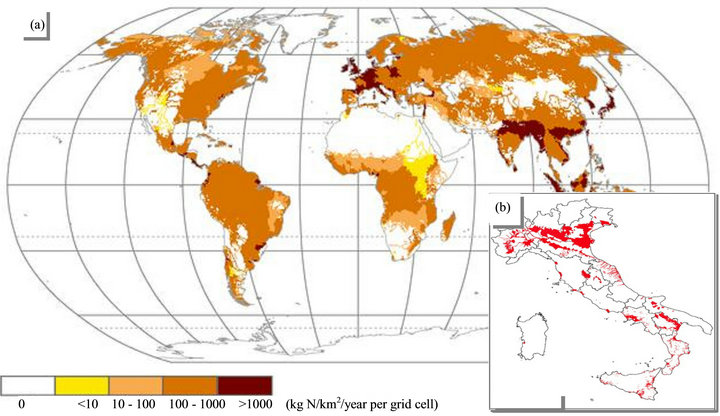
Figure 1. (a) World total nitrogen flux per grid cell (50 × 50 km) (data from http://wwdrii.sr.unh.edu/download.html), and (b) nitrate vulnerable area with concentration above 50 mg∙L−1 (red) in Italy [37].
sector of the wider Campania Plain, a structural depression on the Tyrrhenian Coast (Figure 2(a)). This area, located between Naples (40˚50' North, 14˚15' East) to the East, Somma-Vesuvius (40˚49' North, 14˚25' East) to the South, and the mountains of Sarno (40˚49' North, 14˚37' East) to the North, occupies the south-eastern part of the Campania Plain (Figure 2(b)).
Climate is very variable in spring and autumn and more stable in winter and summer. Dry season, from May to September, not enable to recharge the soil before of November-December, in order to inter-annual variability. A typical seasonal trend of different terms of water balance is illustrated in Figure 3, where the climogram for the Campania Plain describes the humid period (October-March) followed by the dry-summer season (June-August). Transitional periods (April-May and September) are the growing seasons where vegetation is green.
The graben system of the area began to form during the Pliocene, between Mesozoic carbonate sequence outcropping to the east and south of the plain. During the Pleistocene this structural depression was filled with pyroclastic deposits (ashes, pumice, scoriae and tuffs) of Neapolitan volcanoes (Phlegraean Fields and SommaVesuvius) and alluvial (mainly sandy and partly clayey) and marine (mainly silt) sediments to a thickness of some thousands of metres. The first few hundred metres beneath the soil of the circumvesuvian plain, the zone of the most active groundwater circulation, are made up of the pyroclastic deposits (ashes, pumice and scoriae) and alluvial deposits interposed with marine sediments marshy layers and paleosols. The tuff aquitards divide the flow into two overlapping levels (Figure 4).
Travertine, debris and conglomerates lie at the base of the limestone mountains, while approaching the SommaVesuvius volcano lava flows prevail, interbedded with pyroclastic deposits.
The carbonate aquifers are the most important aquifers located at the boundaries of the plain. The Somma-Vesuvius volcano has a radial water table. Groundwater flows towards the sea and also feeds the aquifer of the surrounding plain. The aquifer of the Campania Plain is characteristically extremely heterogeneous due to granulometric variation in the unconsolidated sediments, the degree of fissuring of rock and complex stratification of deposits.
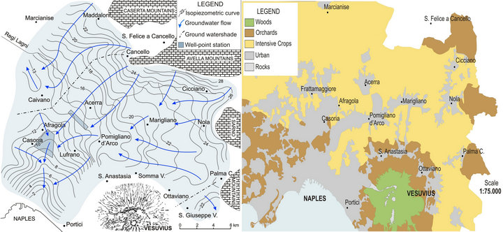
The map (Figure 5(a)) shows that the aquifer of the Campania Plain flows from NE to SW and highlights the presence of one axe of groundwater drainage to the East of Naples. There are two groundwater divides: the first is between San Giuseppe Vesuviano and Palma Campania (in SE of the map) and the second is between Cancello and Caivano (in NW of the map).
The hydraulic gradient varies from a few units per thousand to a few units per hundred. In particular, the highest values of the piezometric gradient found at the foot of Lattari mountains, may be related to high transmissivity from carbonate aquifers (10−1 - 10−2 m2∙s−1) compared with values in other areas the plain (10−2 - 10−4 m2∙s−1).
The main contributions to aquifer recharge are provided by direct infiltration and groundwater inflow from the nearby volcanic and carbonate aquifers. The mean annual effective infiltration is of 59.6 × 10⁶ m3∙yr−1 [23]. In the Figure 5(b) is shown the map of land-use, with the urban and agricultural activity covering most of the study area. The urban areas are developed, however, in the absence of infrastructure networks. Therefore, we assume a deep percolation of organic waste in the aquifer.
2.2. Nitrate Sampling
Groundwater pollution sampling was initiated since 1992
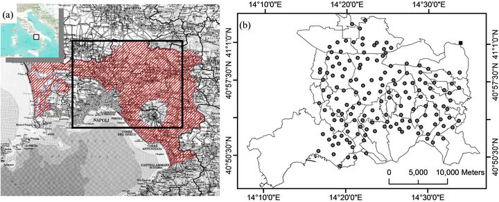
Figure 2. (a) Central coast of Campania region with a suitable zone for nitrate pollution and the study area (squared); (b) Area of investigation with indicated municipalities and wells (dots) where nitrates were sampled. The image in (a) is from Region Campania (http://www.agricoltura.regione.campania.it/nitrati/zvnoana.jpg).
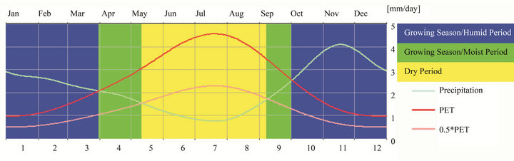
Figure 3. Climogram with representations of the seasonal regime of deficit (yellow band) and surplus water (blue bands) from precipitation for Campania Plain (arranged by New-LocClim FAO software, http://www.fao.org/nr/climpag/pub/en0201_en.asp).
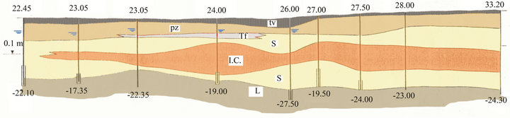
Figure 4. Geological profile of Campania Plain (tv = vegetal soil; pz = pozzolane, tf = tuffs; IC = Ignimbrite Campana; s = sand; l = silt).
 (a) (b)
Figure 5. (a) Map of isopiezometric of groundwater level and (b) land-use cover across the Campania Plain.
in Campania Plain and continued in 2001 and 2006 years [24,25]. However, only in 1992 a wide and resolute sampling was conducted covering a surface of about 500 km2.
In 158 wells used for the reconstruction of the paper in the aquifer isopiezometric curves were also collected water samples for the determination of nitrate concentrations. The analysis refers to the period of low water of the aquifer. Nitrate in water samples was colorimetrically measured [26,27]. The wells were managed by one of the leading institutions of central-southern aqueduct (ARIN, Naples Water Resources Company, http://www.arin.na.it).
2.3. Probability Kriging
Kriging and its derivatives have been recognized as the main spatial interpolation techniques from 1970s. Kriging is a method for making optimal, unbiased estimates of regionalized variables at unsampled points. It is possible to have a good estimation of the selected variable using the values collected in the surrounding stations and a structural analysis [28]. Probability kriging (PK) is a specific method belonging to the family of kriging, introduced by as a non-linear and non-parametric method using indicator variables [29]. PK represents an effort for calculating estimates that are less sensitive than indicator kriging to the choice and number of cut-offs (thresholds) and estimates better reflecting local variability [30]. PK is a composite kriging of the indicator data using the rank-order transform as additional variable [31]. Replacing the values of the primary variable in PK by indicator data and using the rank-order transform data, the indicator code,  , is assigned as the pollutant variable [32,33]. A vector-based GIS software package ArcGIS 9.2 was used to map, query, and analyze the data in this study.
2.4. Decision-Making in the Presence of Uncertainty
In the present paper, environmental risk assessments related to nitrate pollution are derived from the probability that a pollutant leaching rate can migrate from sub-surface to groundwater. The selected thresholds or the action level often determine the introduction or not of certain measures. The concentration in natural water is less than 10 mg∙L−1. Water containing more than 100 mg∙L−1 is bitter to taste and causes physiological distress. Water in shallow wells containing more than 50 mg∙L−1 causes methemoglobinemia, the so-called blue baby syndrome in humans [34].
Availability of the regionalization between indicator pollutant at nitrate threshold concentrations for each location sα within the study area would allow a grid layer α(sα) referring to “probable hydrogeological effectiveness” of the nitrate pollutant on the basis of the estimate  when actually
 . The European Commission suggested two limits for nitrates: a first threshold, zk1 = 25 mg∙L−1, which represents the minimum concentration needed to overcome the drinking groundwater quality, and the second, zk2 = 50 mg∙L−1, which represents the maximum values for the drinking groundwater quality.
3. Results and Discussion
The ability to identify the true spatial variability of a dataset depends to a great extent, on ancillary knowledge of the underlying measured phenomenon. This is why exploratory data analysis is often the first step in hydrogeostatistical studies. Postplot, initial contour maps and basic statistics are used as a preliminary description of the dataset in a spatial context and to develop a strategy for future evaluation [35].
3.1. Distribution of the Data
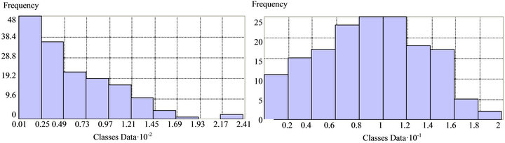
The presence of nitrates is considered an indicator of pollution in the Campania Plain because of the intensive agricultural land use, urbanization and industrial practices throughout the area. In several wells, nitrate concentrations exceed the maximum allowable concentration (50 mg∙L−1) as set by the Italian law. The statistics of nitrate data collected in October 1993 are summarized with mean and median values equal to 57 mg∙L−1, and 43 mg∙L−1, respectively. The maximum value is 239 mg∙L−1. Figure 6(a) shows a strong skewed distribution. This is why a Box-Cox transformation (with 0.4 transformation parameter) was adopted. The transformation results in a quasinormal distribution (Figure 6(b)).
3.2. Spatial Structural Modelling
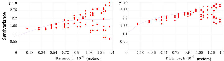
A two-stage model of regionalization was fitted using an iterative procedure [31]. Stage 1 assumes an isotropic model and executes a first run of the experimental spatial structures on the scaled data,  , where z(sα) is used to denote the jth measurement of a variable at the αth spatial locations sα, and σ is the sample standard deviation. With stage 2, numbers such as lag (assumed equal 7), lag size h (assumed equal to 2000 m), and range (a) are set to represent the limit of spatial dependence, while nugget is set to represent the unexplained spatial variability, calibrated interactively. Also at, this stage it has been assumed an isotropic semivariogram model for the pollutant indicator spatial pattern. In this way, Figure 7 shows the experimental semivariogram (dots) computed from 158 nitrate data, with spherical permissible models fitted (blue curves).
Semivariogram values increase with the separation distance, reflecting the assumption that nearby nitrate-pollutant data tend to be more similar than data that are farther apart. The modelled variograms have been tested by the cross-validation method. The semivariograms reach 2000 to 10,000 m before dipping around a sill value.
 (a) (b)
Figure 6. (a) Statistical distribution of nitrate concentration for the original series and (b) Box-Cox transformed series (nitrate classes data along X-axis are in mg∙L−1).
 (a) (b)
Figure 7. (a) Experimental semivariance (dots) and related spherical models (curves) for zk > 25 mg∙L−1), and (b) for zk > 50 mg∙L−1). The semivariogram in (b) is composed by nugget effect plus two spherical structures.
In particular, while unidirectional semivariograms in Figure 7(a) was modelled as a combination of two distinct spatial structures-nugget variance and a spherical structure for zk1—the semivariogram in Figure 7(b) was composed by nugget plus two spherical structures for zk2 (Figure 6(b)) (see also Equations (3) and (4)).
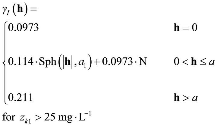 (3)
(3)
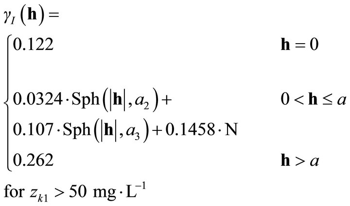 (4)
(4)
The three spatial structures for high nitrate concentration lead us to believe that there are different sources of pollution resulting from the landscape overlying the aquifer. At the local level the presence of nitrates may result from direct leakage into the groundwater of organic waste. At larger range, instead, nitrate may have derived from non-point source as agricultural manures.
The symbolic term in Equations (3) and (4),  , is the spherical correlation function equal to
 .
.
It represents a dimensional semivariance of unit sill with ranges given by the circle with a1 = 10000, zk1 = 25 mg∙L−1, and a2 = 3000 a3 = 10000 meters, for zk2. Ideally, the value of the semivariogram should reach a minimum value when the separation vector h is zero. In the case study, this is not true firstly because the measurement error exists in nitrate sampling data, and secondly because the distribution and number of wells could be poor. The range relative to the large threshold, zk2 = 50 mg∙L−1, has a minor nugget than with zk1 = 25 mg∙L−1 but the nugget/total sill ratio is roughly the same (0.46 - 0.47)which indicates moderate spatial correlation for both the thresholds.
3.3. Spatial Pattern of Estimation and Hazard Classification
Figures 8(a) and (b) show probability-kriged maps, based on 500 m by 500 m grid across Campania Plain. In kriged model pattern area of Figure 8(a), it is possible to observe a distinct separation between East (minor) and West (major) zone of nitrate map, which is consistent with the pattern of groundwater flow outlined in par. 2.1. The areas having probability of 50% that the nitrate concentration exceeded 25 and 50 mg∙L−1 are narrow, intermediate bands (in light blue). This indicates that nitrate concentration is characterized by high gradient when its concentration is near the threshold values.
Especially in the map of Figure 8(a), it appears a distinct separation between little free zone at East (blue) and a large polluted area at West (red-orange-yellow) including Naples metropolitan area. This map accounts for areas exceeding 25 mg∙L−1 for about 70% of the total surface.
In Figure 8(b), it is mapped the probability that nitrate concentration exceeded the 50 mg∙L−1, with high probability that remains at West, although not all areas are strongly polluted. In this case, areas with very high probability are aligned along a diagonal line crossing Maddaloni, Acerra, Lufrano and Naples municipalities.
As already outlined [24], this trend takes into account the groundwater inflow that is carried out in correspondence of the foothills (cf. par. 2.1), but also the concentration of the pollutant that originates from the surface and effective infiltration. Due to the source of surface contamination, the pollutant load in the vicinity of the foothills is not particularly high, when compared to that of more central areas of the plain. This is due both to the limited extension of the foothills, on which the effective infiltration of rain takes place, and to a major capacity of denitrification of the plain subject to agricultural manure. In the most central part of the plain, there has been a general increase in the spread of nitrates due to the flow of water and potential pollution. Comparing land-use chart and nitrate probability maps, we can see an increase in hazard only where intensive agriculture mixes with more urbanized areas.
At the time of sampling, the only areas remaining free from high concentrations can be individuated between the surrounding of Palma Campania, Nola, Marigliano and Roccarainola municipalities. Local patterns with high nitrate concentration were also founded in Somma Vesuviana and Palma Campania, especially in PK [>50 mg∙L−1].
However, no spatial pattern variability can be detected below 2000 m, due to nugget effect. This represents unexplained or random variance, which is either caused by variability of data that cannot be detected at the scale of sampling, or measurement errors within Campania Plain. Although the monitoring phase refers to the period of lean ground when less effective infiltration is present, the maps presented here suggest a dramatic pattern with still high probability of exceeding the above limits. Therefore, it is suspected that nitrate concentrations in well water can be high during any month of the year and the issue of nitrate contamination and health effects should not be ignored.
3.4. Cross-Validation Results and Spatial Error Qualitative Assessment
The error involved on the expansion of the information from point to landscapes through probability kriging es-
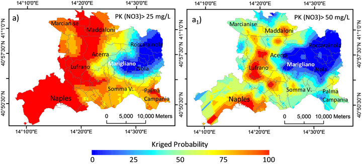
Figure 8. Spatial patterns of kriged-probability maps exceeding the nitrate threshold-value of (a) 25 mg∙L−1, and (b) 50 mg∙L−1 across Campania Plain for October 1992.
timation can be assessed through a quantitative estimation standard error of indicator and cross-validation [36].
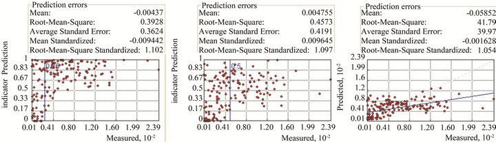
The result of the cross-validation is presented within the statistical errors and scatter diagram (above and below panels in Figure 9, respectively). Mean is minor of 0.01 for PK [(a) and (b)] showing lack of systematic error. Since Root Mean Square Error is close to the Average Standard Errors (second and third row, respectively, in Figures 8(a) and (b)), mean is correctly assessing the variability in prediction. Root Mean Square Standardized error (RMSS) compare the error variance with the same theoretical variance such as kriging variance. Therefore, it should be close to 1, as resulting from the fifth row, where RMSS is 1.01.
If we consider OK experiment, measurements versus the predicted values of nitrate are in disagreement (see the scatter diagram of Figure 9(c)). Also, mean error is greater than 0.01, although the other errors are comparable with PK approach. However, a large bias remains in the relative scatter plot, indicating that OK is not suitable for interpreting spatial pattern in Campania Plain.
4. Discussion and Conclusions
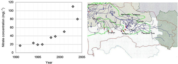
Figure 10 shows that nitrate concentrations have increased compared to the first sampling in 1993. Analyzing both the graphs of Figure 10(a), it appears that nitrate concentration has increased both in time and in space. Therefore, a strong temporal persistence and enrichment of nitrate concentrations seems to be present in the aquifer. However the few sampling points of 2006 (black dots in Figure 10(b)) does not allow us to compare the relative map with the one developed in this work.
This study has attempted to predict the spatial distribution and uncertainty of groundwater nitrate concentration across some municipalities of the Campania Plain (Southern Italy). Probability kriging, a type of nonparametric geostatistical techniques, was applied to the groundwater nitrate hazard data for two distribution maps related to
 (a) (b) (c)
Figure 9. Scatterplot of cross-validation between nitrate-measured and indicator probability kriging for the nitrate-thresholds of (a) 25 mg∙L−1, and (b) 50 mg∙L−1, and (c) for ordinary kriging. Vertical lines in both graphs (a) and (b) represent the respective thresholds. In graph (c), a large bias exists for ordinary kriging application.
 (a) (b)
Figure 10. (a) Trend of nitrate concentration in Somma Vesuviana from 1991 to 2004 [38], and (b) iso-nitrate pattern upon Campania Plain in 2006 (from ENEA, http://eboals.bologna.enea.it/ambtd/regi-lagni/volume-2/3-vol2-ac_sot_all6.html).
the threshold values of 25 and 50 mg∙L−1, respectively. Geostatistics can provide tools to describe spatial and hazard behavior of hydrochemical parameters. Groundwater nitrate concentrations were log-normally distributed. The spherical model was found to be the best model representing the spatial variability of groundwater probability nitrate maps. The average value of the variograms for the spatial analysis was in a range of 2000 - 10,000 m in the spherical model. Nitrate pollution in the groundwater occurred most in the urban and periurban centre of the municipalities because of nitrate excess from biological, agricultural and, secondarily, industrial production. Although the modelling results indicate that the probability kriged groundwater nitrate maps satisfactorily matched the observed groundwater nitrate distribution, a newer and more continuos sampling is needed for reaching the areas with more hazard.
REFERENCES
- S. Buchan and A. Key, “Pollution of Ground Water in Europe,” Bulletin of the World Health Organization, Vol. 14, No. 5-6, 1956, pp. 949-1006.
- T. Huang, Z. Pang and W. M. Edmunds, “Soil Profile Evolution Following Land-Use Change: Implications for Groundwater Quantity and Quality,” Hydrological Processes, Vol. 27, No. 8, 2012, pp. 1238-1252. doi:10.1002/hyp.9302
- A. Visser, I. Dubus, H. P. Broers, S. Brouyere, M. Korcz, P. Orban, P. Goderniaux, J. Batlle-Aguilar, N. Surdyk, N. Amraoui, H. Job, J. L. Pinault and M. Bierken, “Comparison of Methods for the Detection and Extrapolation of Trends in Groundwater Quality,” Journal of Environmental Monitoring, Vol. 11, No. 11, 2009, pp. 2030-2043. doi:10.1039/b905926a
- J. K. Böhlke, “Groundwater Recharge and Agricultural Contamination,” Hydrogeology Journal, Vol. 10, No. 1, 2002, pp. 153-179. doi:10.1007/s10040-001-0183-3
- M. de Wit, H. Behrendt, G. Bendoricchio, W. Bleuten and P. van Gaans, “The Contribution of Agriculture to Nutrient Pollution in Three European Rivers, with Reference to the European Nitrates Directive,” European Water Management Online, 2002. www.ewaonline.de/journal/2002_02.pdf
- G. J. Kraft and W. Stites, “Nitrate Impacts on Groundwater from Irrigated-Vegetable Systems in a Humid NorthCentral US Sand Plain,” Agriculture, Ecosystems and Environment, Vol. 100, No. 1, 2003, pp. 63-74. doi:10.1016/S0167-8809(03)00172-5
- B. Nas and A. Berktay, “Groundwater Contamination by Nitrates in the City of Konya (Turkey): A GIS Perspective,” Journal of Environmental Management, Vol. 79, No. 1, 2006, pp. 30-37. doi:10.1016/j.jenvman.2005.05.010
- J. J. Schröder, D. Scholefield, F. Cabral and G. Hofman, “The Effects of Nutrient Losses from Agriculture on Ground and Surface Water Quality: The Position of Science in Developing Indicators for Regulation,” Environmental Science & Policy, Vol. 7, 2004, pp. 15-23. doi:10.1016/j.envsci.2003.10.006
- S. Chand, M. Ashif, M. Y. Zargar and B. M. Ayub, “Nitrate Pollution: A Menace to Human, Soil, Water and Plant,” Universal Journal of Environmental Research and Technology, Vol. 1, 2011, pp. 22-32.
- J. A. Vomocil, “Fertilizers: Best Management Practices to Control Nutrients,” Proceedings of the Northwest Nonpoint Source Pollution Conference, Olympia, 24-25 March 1987, pp. 88-97.
- G. R. Hallberg and D. R. Keeney, “Nitrate,” In: W. M. Alley, Ed., Regional Groundwater Quality, van Nostrand Reinhold, New York, 1993, pp. 297-322.
- I. Lord, S. G. Anthony and G. Goodlass, “Agricultural Nitrogen Balance and Water Quality in the UK,” Soil Use and Management, Vol. 18, No. 4, 2006, pp. 363-369. doi:10.1111/j.1475-2743.2002.tb00253.x
- C. D. Rail, “Groundwater Contamination: Sources, Control, and Preventive Measures,” Technomic, Lancaster, 1989.
- C. J. Johnson, P. A. Bonrud, T. L. Dosch, A. W. Kilness, K. A. Senger, D. C. Busch and M. R. Meyer, “Fatal Outcome of Methemoglobinemia in an Infant,” Journal of the American Medical Association, Vol. 257, No. 20, 1987, pp. 2796-2797. doi:10.1001/jama.1987.03390200136029
- S. M. Kharad, K. Srinivas Rao and G. S. Rao, “GIS Based Groundwater Assessment Model,” GIS@development, 1999. http://www.gisdevelopment.net/application/nrm/water/ground/watg0001.htm
- M. Butler, J. Wallace and M. Lowe, “Ground-Water Quality Classification Using GIS Contouring Methods for Cedar Valley, Iron County, Utah,” US Geological Survey Open-File Report 02-370, Workshop Proceedings of Digital Mapping Techniques, Salt Lake City, 19-22 May 2002.
- S. S. Asadi, P. Vuppala and M. A. Reddy, “Remote Sensing and GIS Techniques for Evaluation of Groundwater Quality in Municipal Corporation of Hyderabad (Zone-V), India,” International Journal of Environmental Research and Public Health, Vol. 4, No. 1, 2007, pp. 45-52. doi:10.3390/ijerph2007010008
- P. Balakrishnan, A. Saleem and N. D. Mallikarjun, “Groundwater Quality Mapping Using Geographic Information System (GIS): A Case Study of Gulbarga City, Karnataka,” India African Journal of Environmental Science and Technology, Vol. 5, No. 12, 2011, pp. 1069- 1084.
- R. A. Carlson and J. L. Osiensky, “Geostatistical Analysis and Simulation of Nonpoint Source Groundwater Nitrate Contamination: A Case Study,” Environmental Geoscience, Vol. 5, No. 4, 1998, pp. 177-186.
- C. W. Liu, C. S. Jang and C. M. Liao, “Evaluation of Arsenic Contamination Potential Using Indicator Kriging in the Yun-Lin Aquifer (Taiwan),” Science of the Total Environment, Vol. 321, No. 1-3, 2004, pp. 173-188. doi:10.1016/j.scitotenv.2003.09.002
- N. Diodato and M. Ceccarelli, “Computational Uncertainty Analysis of Groundwater Recharge in Catchment,” Ecological Informatics, Vol. 1, No. 4, 2006, pp. 377-389. doi:10.1016/j.ecoinf.2006.02.003
- C. Piccini, A. Marchetti, R. Farina and R. Francaviglia, “Application of Indicator Kriging to Evaluate the Probability of Exceeding Nitrate Contamination Thresholds,” International Journal of Environmental Research, Vol. 6, No. 4, 2012, pp. 853-862.
- L. Esposito and V. Piscopo, “Groundwater Flow Evolution in the Circum-Vesuvian Plain (Italy),” Proceedings of the XXVII IAH Congress on Groundwater in the Urban Environment, Nottingham, 21-27 September 1997, pp. 309-314.
- F. Celico, L. Esposito and V. Piscopo, “Limiti di Applicabilità Delle Carte Della Vulnerabilità All’Inquinamento Degli Acquiferi Nella Previsione Dello Stato di Contaminazione Antropica Delle Acque Sotterranee,” Geologica Romana, Vol. 33, 1997, pp. 65-72 (in Italian).
- A. Corniello and D. Ducci, “Origine Dell’Inquinamento da Nitrati Nelle Falde Dell’Area di Acerra (Piana Campana),” Engineering Hydro Environmental Geology, Vol. 12, 2009, pp. 157-166 (in Italian).
- M. J. Fishman and L. C. Friedman, “Methods for Determination of Inorganic Substances in Water and Fluvial Sediments,” US Geological Survey Techniques of WaterResources Investigations, Book 5, Chapter A1, 1989.
- M. J. Fishman, “Methods of Analysis by the US Geological Survey National Water Quality Laboratory-Determination of Inorganic and Organic Constituents in Water and Fluvial Sediments,” US Geological Survey Open-File Report, 1993, pp. 93-125.
- A. G. Journel and C. J. Huijbregts, “Mining Geostatistics,” Academic Press, New York, 1978.
- J. Sullivan, “Conditional Recovery Estimation through Probability Kriging-Theory and Practice,” In: G. M. Verly, M. David, A. G. Journel and A. Marechal, Eds., Geostatistics for Natural Resources Characterisation, Part 1., Reidel, Dordrecht, 1984, pp. 365-384. doi:10.1007/978-94-009-3699-7_22
- M. E. Hohn, “Petroleum and Geostatistics,” Kluwer Academic Publishers, Dordrecht, 1999.
- P. Goovaerts, “Geostatistics for Natural Resources Evaluation,” Oxford University Press, New York, 1997.
- C. V. Deutsch and A. G. Journel, “GSLIB Geostatistical Software Library and User’s Guide,” Oxford University Press, New York, 1992.
- K. Johnston, J. M. Ver Hoef, K. Krivoruchko and N. Lucas, “Using ArcGis Geostatistical Analyst,” ESRI, 2001.
- P. Balakrishnan, A. Saleem and N. D. Mallikarjun, “Groundwater Quality Mapping Using Geographic Information System (GIS): A Case Study of Gulbarga City, Karnataka, India,” African Journal of Environmental Science and Technology, Vol. 5, No. 12, 2011, pp. 1069- 1084.
- R. Carlson and J. Osiensky, “Geostatistical Analysis and Simulation of Nonpoint Source Groundwater Nitrate Contamination: A Case Study,” Environmental Geosciences, Vol. 5, No. 4, 1998, pp. 177-186. doi:10.1046/j.1526-0984.1998.08025.x
- E. H. Isaaks and R. M. Srivastava, “An Introduction to Applied Geostatistics,” Oxford University Press, New York, 1989.
- E. Capri, M. Civita, A. Corniello, G. Cusimano, M. De Maio, D. Ducci, G. Fait, A. Fiorucci, S. Hauser, A. Pisciotta, G. Pranzini, M. Trevisan, A. Delgado Huertas, F. Ferrari, R. Frullini, B. Nisi, M. Offi, O. Vaselli and M. Vassallo, “Assessment of Nitrate Contamination Risk: The Italian Experience,” Journal of Geochemical Exploration, Vol. 102, No. 2, 2009, pp. 71-86. doi:10.1016/j.gexplo.2009.02.006
- G. Onorati and T. Di Meo, “Lo Stato Delle Acque Sotterranee in Campania e la Diffusione dei Nitrati. La Direttiva Nitrati, Un’Opportunità per L’Agricoltura Campana,” ARPAC, Convegno Provinciale Avellino, 21 giugno 2006 (in Italian). http://www.stapacepicaavellino.com/documenti/nitrati/onorati-dimeo.pdf
NOTES
*Corresponding author.