Open Journal of Applied Sciences
Vol.4 No.9(2014), Article ID:48746,19 pages
DOI:10.4236/ojapps.2014.49046
Epistasis in Predator-Prey Relationships
Iuliia Inozemtseva, James Braselton*
Georgia Southern University, Statesboro, GA, USA
Email: ii00073@georgiasouthern.edu, *jbraselton@georgiasouthern.edu
Received 5 June 2014; revised 23 July 2014; accepted 8 August 201 4
ABSTRACT
Epistasis is the interaction between two or more genes to control a single phenotype. We model epistasis of the prey in a two-locus two-allele problem in a basic predator-prey relationship. The resulting model allows us to examine both population sizes as well as genotypic and phenotypic frequencies. In the context of several numerical examples, we show that if epistasis results in an undesirable or desirable phenotype in the prey by making the particular genotype more or less susceptible to the predator or dangerous to the predator, elimination of undesirable phenotypes and then genotypes occurs.
Keywords:Epistasis, Predator-Prey Equations, Logistic Equation, Hardy-Weinberg Equation

1. Introduction
The usual starting point for models in population genetics is a model of random
mating for a one-locus, twoallele problem with Hardy-Weinberg proportions for the
alleles. Refer to Karlin [1] , for an overview
of mathematical models of population genetics. In genetic problems, the genotype
is defined to be the genetic makeup of an organism. For example, in a one-locus,
two-allele model, one can label the alleles as
 (dominant) and
 (recessive). The possible genotypes are then
 ,
,
![]() , and
, and . On the other hand, the phenotype is defined
to be the set of observable characteristics of an individual resulting from the
interaction of its genotype with the environment. In the absence of epistasis, defined
in the next paragraph, with the above genotypes, the phenotypes would be
. On the other hand, the phenotype is defined
to be the set of observable characteristics of an individual resulting from the
interaction of its genotype with the environment. In the absence of epistasis, defined
in the next paragraph, with the above genotypes, the phenotypes would be
 for the genotypes of type
 and
and
![]() and
and
 for the genotype of type
 .
.
Epistasis occurs when the genotype results in a phenotype different from that expected.
For example, in the context of the example above, epistasis would occur if either
the
 or
or
![]() genotype did not result in the phenotype expected,
genotype did not result in the phenotype expected, .
.
One of the more interesting examples of epistasis in humans occurs in human blood
in the form of the Bombay Phenotype. The Bombay Phenotype is a very rare blood phenotype
in humans that is scientifically referred to as the
 (the
(the ) antigen that results in a phenotype of type
![]() , even though the genotype of these individuals
is of type
, even though the genotype of these individuals
is of type![]() , which typically would be expressed as of type
, which typically would be expressed as of type . People with the Bombay Phenotype can donate to
any member of the
. People with the Bombay Phenotype can donate to
any member of the
![]() blood group system, but they can only receive blood from others with the Bombay
Phenotype. The Bombay Phenotype is very rare and only occurs in approximately 1
in 10,000 individuals in India and 1 in a million people in Europe (see [2] ).
blood group system, but they can only receive blood from others with the Bombay
Phenotype. The Bombay Phenotype is very rare and only occurs in approximately 1
in 10,000 individuals in India and 1 in a million people in Europe (see [2] ).
In the study of epistasis discussed here the modifications introduced are that epistasis is incorporated into a standard predator-prey model, so that one genotype of the prey may be more or less susceptible to the predator than other prey with a different genotype, but the same phenotype in the absence of epistasis. Second, we introduce epistasis in the standard predator-prey model so that one genotype of the prey is dangerous (lethal or poisonous) to the predator than other prey with different genotypes but the same expected phenotype in the absence of epistasis.
This is accomplished by a perturbation of the random mating model within the context of established ecological models for the evolution of a predator-prey population.
Of course, general mating preferences almost certainly depend on numerous external factors that might include but are not limited to available mates, parasites, season, climate, and such that they are beyond the scope of the model discussed here, but could lead to interesting extensions of the situations discussed here.
2. Formulation of the Model
2.1. The Standard Predator-Prey Equations
Let
 denote the size or density of the prey population and
 denote the size or density of the predator population. Then the standard predator-prey
equations take the form
denote the size or density of the predator population. Then the standard predator-prey
equations take the form
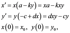 (1)
(1)
where ,
,
 ,
,
 , and
, and
 are all positive constants. Refer to Lotka [3]
, or Karlin [1] , for basic details regarding the
standard Predator-Prey model. In the absence of the predator, the prey has linear
growth, given by the
are all positive constants. Refer to Lotka [3]
, or Karlin [1] , for basic details regarding the
standard Predator-Prey model. In the absence of the predator, the prey has linear
growth, given by the
 term. The death rate of the prey is governed by predator-prey interactions given
by the quadratic
term. The death rate of the prey is governed by predator-prey interactions given
by the quadratic
 term, which contributes to the growth rate of the predator by the
 term. We interpret
 to be the catchability of the prey
 by the predator
![]() . Details regarding the standard predator-prey
equations and different interpretations of the coefficients are discussed in most
introductory differential equations texts like Abell and Braselton [4] , or introductory mathematical modeling and/or mathematical
biology texts such as Beltrami [5] , or Murray
[6] .
. Details regarding the standard predator-prey
equations and different interpretations of the coefficients are discussed in most
introductory differential equations texts like Abell and Braselton [4] , or introductory mathematical modeling and/or mathematical
biology texts such as Beltrami [5] , or Murray
[6] .
The most important result for system (1) is that the equilibrium (rest) point
 is classified as a center in the corresponding linearized system because the eigenvalues
of the Jacobian of system (1),
is classified as a center in the corresponding linearized system because the eigenvalues
of the Jacobian of system (1),

evaluated at the equilibrium (rest) point
 are
are
While the stability of the equilibrium point in the nonlinear system is generally
inconclusive in this case, other solution methods can verify that the equilibrium
point is, in fact, a center. A typical example is shown in
Figure 1, where we have used the values![]() ,
,
 ,
,
![]() , and
, and . In Figure 1,
observe how the limit cycles revolve about the center,
. In Figure 1,
observe how the limit cycles revolve about the center,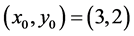 .
.
Figure 1.
We choose![]() ,
,
![]() ,
,
![]() , and
, and![]() . Observe how the solution curves revolve about
the center,
. Observe how the solution curves revolve about
the center, .
.
2.2. A Two-Locus, Two-Allele Model
In the two-locus, two-allele problem, the number of genotypes is nine but in the
absence of epistasis, the number of phenotypes is four. If the
 and
and
 alleles are dominant, the expected result is four phenotypes
 (
( ,
,![]() ,
,
![]() , and
, and![]() ),
),
 (
( and
and![]() ),
),
![]() (
(![]() and
and ), and
 (
(![]() ), as described next. For the two-locus, two-allele problem,we
consider a population
), as described next. For the two-locus, two-allele problem,we
consider a population
 with size (or density)

where
•
 is the size of the population of type
 (expected phenotype
 )•
)•
![]() is the size of the population of type
is the size of the population of type
 (expected phenotype
 )•
)•
 is the size of the population of type
 (expected phenotype
 )•
)•
![]() is the size of the population of type
is the size of the population of type
![]() (expected phenotype
(expected phenotype )•
)•
![]() is the size of the population of type
is the size of the population of type
 (expected phenotype
 )•
)•
![]() is the size of the population of type
is the size of the population of type
 (expected phenotype
 )•
)•
![]() is the size of the population of type
is the size of the population of type
![]() (expected phenotype
(expected phenotype![]() )•
)•
 is the size of the population of type
 (expected phenotype
![]() ) and
) and
•
![]() is the size of the population of type
is the size of the population of type
 (expected phenotype
 ).
).
The proportion of gametes of type ,
,
 ,
,
![]() , and
, and
 are given by
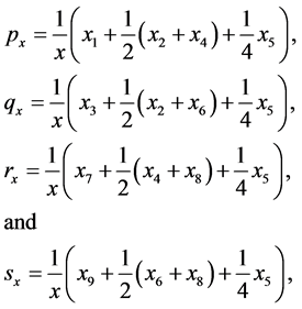 (2)
(2)
respectively. Observe that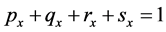 . Table A1
in the Appendix shows the expected ratio of offspring
produced by each
. Table A1
in the Appendix shows the expected ratio of offspring
produced by each
 combination. Refer to articles like Braselton et al. [7]
, or Szathmáry [8] , for details regarding these
and similar calculations.
combination. Refer to articles like Braselton et al. [7]
, or Szathmáry [8] , for details regarding these
and similar calculations.
Assuming random mating between the genotypes of the prey, the predator-prey Equations (1) become
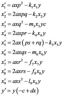 (3)
(3)
with initial conditions
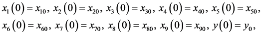 (4)
(4)
where we have used Table A1 in the Appendix to compute the coefficients and simplified the results
using Equation (2) as well as omitted the subscripts for the ,
,
 ,
,
 , and
, and
 terms.
If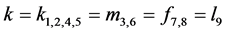 , adding system (3) and then substituting the proportion of
gametes given in Equation (2) and adding
, adding system (3) and then substituting the proportion of
gametes given in Equation (2) and adding
 results in the predator-prey equations, system (1). Using Equation (2), the allele
frequencies of
results in the predator-prey equations, system (1). Using Equation (2), the allele
frequencies of ,
,
 ,
,
 , and
, and
 are given by
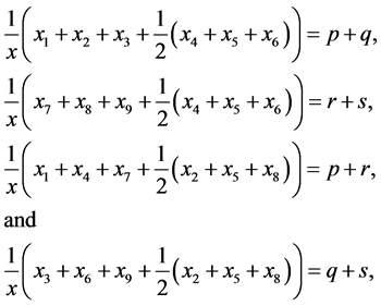 (5)
(5)
respectively.
In addition, using system (3) and Equations (2), we have
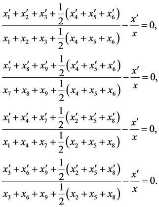 (6)
(6)
Integrating and exponentiating each Equation in (6) results in the following
 (7)
(7)
This proves the theorem.
Theorem 1. For random mating, the relative frequencies of the alleles ,
,
 ,
,
 , and
, and
 are constant, agreeing with the Hardy-Weinberg equation.
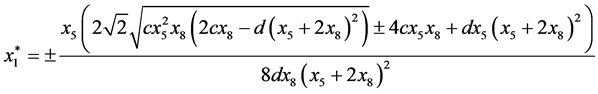
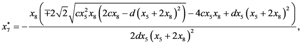
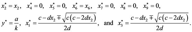
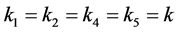
Theorem 2. If , there are up to 14 equilibrium (rest) points,
provided that the appropriate quantities are nonnegative.
, there are up to 14 equilibrium (rest) points,
provided that the appropriate quantities are nonnegative.
Proof. In the following,
 ,
,
 ,
,
 ,
,
 ,
,
 ,
,
 ,
,
 ,
,
 , and
, and .
.
 are given by


and

Next,
 are given by


 are given by
 are given by
 are given by
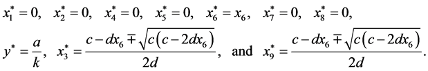
 is given by
 ,
,
 ,
,
 ,
,
 ,
,
 ,
,
 ,
,
 ,
,
 ,
,
 , and
, and .
.
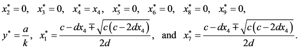
 is given by
 ,
,
 ,
,
 ,
,
 ,
,
 ,
,
 ,
,
 ,
,
 ,
,
 , and
, and .
.
 is given by
 ,
,
 ,
,
 ,
,
 ,
,
 ,
,
 ,
,
 ,
,
 ,
,
 , and
, and .
.
Finally,
 is given by
 ,
,
 ,
,
 ,
,
 ,
,
 ,
,
 ,
,
 ,
,
 ,
,
 , and
, and .
.
For all 14 rest points, .
.
Observe that the Jacobian,
![]() , for system (3) is a
, for system (3) is a
![]() matrix. We are unable to compute the eigenvalues of
matrix. We are unable to compute the eigenvalues of
![]() at
at
![]() or
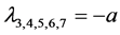
or . However, for the remaining rest points (equilibrium points),
 ,
,
 ,
,
![]() ,
,
 , the eigenvalues of
![]() evaluated at
evaluated at
![]() are
are ,
,
 ,
,
 , and
, and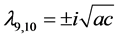 . Thus, we expect the rest points to usually
be “center-like”, which is illustrated in the computations.
. Thus, we expect the rest points to usually
be “center-like”, which is illustrated in the computations.
When
 (phenotype
 ),
),
 (phenotype
 ), or
), or
 (phenotype
![]() ), the interpretation is that the corresponding phenotype
of the prey have the same catchability to the predator. In this situation, we are
not able to find exact formulas for the rest points as in the case when
), the interpretation is that the corresponding phenotype
of the prey have the same catchability to the predator. In this situation, we are
not able to find exact formulas for the rest points as in the case when
 . Thus, we conduct numerous numerical studies to explore some
of the possibilities.
. Thus, we conduct numerous numerical studies to explore some
of the possibilities.
When all parameter values have similar values as in the standard predator-prey Equation (1), we typically see a limit cycle that is illustrated in Figure 2.
Reviewing the standard predator-prey system of Equation (1), we expect to see that
the higher parameter values of
 and
and
 (such as
![]() and
and![]() ) give the advantage to the prey because the parameter
) give the advantage to the prey because the parameter
 is the growth rate of the (prey) species
 and the parameter
 is the death (or emigration) rate of (predator) species
![]() .
.
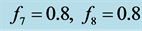
With these parameter values, Figure 3 illustrates
that the genotype
 generally has the highest population sizes/densities. Because
 matings produce all of the other genotypes, all genotypes and phenotypes,
 ,
,
 ,
,
![]() and
and
 coexist.
Choosing values for
 and
and
 to be greater than values for
 and
and
 (using the same initial conditions and values for
 ,
,
 , and
, and
 in (1)) causes the two-locus, two-allele problem to typically result in a stable
solution, such as the stable equilibrium point illustrated in
Figure 4 and Figure 5.
in (1)) causes the two-locus, two-allele problem to typically result in a stable
solution, such as the stable equilibrium point illustrated in
Figure 4 and Figure 5.
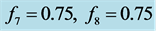
Giving the “weakest” genotype, usually the genotype of type
 (expected phenotype is
 ), an advantage with a low catchability rate
with respect to the other genotypes, such as
), an advantage with a low catchability rate
with respect to the other genotypes, such as , helps this genotype to persist, even with relatively
low population size/density. Regardless, in this simulation the genotype of type
, helps this genotype to persist, even with relatively
low population size/density. Regardless, in this simulation the genotype of type
 again has the highest population density as illustrated in
Figure 6.
again has the highest population density as illustrated in
Figure 6.
From Figure 6 we see the stabilization points (or
equilibrium or rest points) for the predator and prey populations. In Figure 7, the population density for the prey (black) converges
to
![]() and the population
and the population
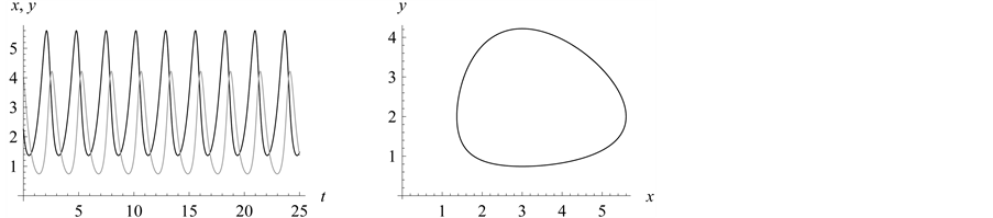
Figure 2. We choose
 and
and . Initial values are
 . All solutions, except for the equilibrium
solution
. All solutions, except for the equilibrium
solution![]() ,
,
 , are periodic so all solution curves are closed curves in
the graph on the right.
, are periodic so all solution curves are closed curves in
the graph on the right.
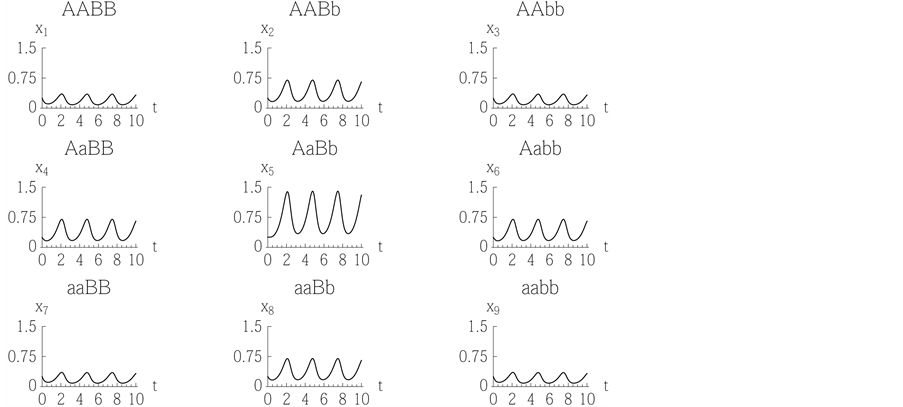
Figure 3. Because the genotype
of type
![]() has an advantage over the others, all genotypes coexist because random matings of
this genotype produce all other genotypes (refer to the
Appendix).
has an advantage over the others, all genotypes coexist because random matings of
this genotype produce all other genotypes (refer to the
Appendix).
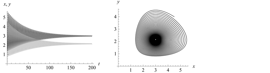
Figure 4. The parameter
values used are![]() ,
,
![]() ,
,
 and
and![]() , which result in stabilization.
, which result in stabilization.
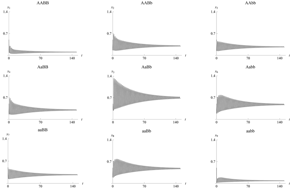
Figure 5. Stabilization
with![]() ,
,
![]() ,
,
 and
and![]() . The size/density of the population of each
expected phenotype stabilizes.
. The size/density of the population of each
expected phenotype stabilizes.
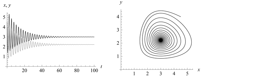
Figure 6. Stabilization
with![]() ,
,
![]() ,
,
 and
and![]() .
.
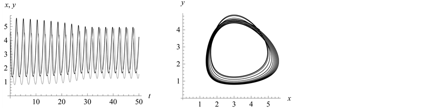
Figure 7. A limit cycle with![]() ,
,
 and
and![]() .
.
density of the predator (grey) converges to .
.
Our final example using this model illustrates that when the expected weakest genotype
of type,
 , dominates, both the
 and
and
 alleles may go to fixation (In the gene pool, fixation means that of two variants
of a particular allele (gene), only one of the alleles remains after a period of
time). Refer to Figure 7. Both prey and predator
populations/densities remain at almost oscillatory rates as shown in the graph on
the left in Figure 7.
alleles may go to fixation (In the gene pool, fixation means that of two variants
of a particular allele (gene), only one of the alleles remains after a period of
time). Refer to Figure 7. Both prey and predator
populations/densities remain at almost oscillatory rates as shown in the graph on
the left in Figure 7.
In Figure 8, observe that we expected the “strongest”
(lowest mortality rate than the other prey genotypes experience with the predator)
genotypes to survive, but their population rates were continuously decreasing. At
some point, around , all vanish. At the same time, the population
density of the
, all vanish. At the same time, the population
density of the
 genotype type starts to increase and stabilizes in the range from 1.8 to 5: the
 and
and
 alleles go to fixation.
3. Epistasis
As discussed previously, epistasis occurs when the genotype results in a phenotype
different from that expected. We model epistasis in a predator-prey relationship
by forcing the catchability (given by the ,
,
 , or
, or
 terms) of one genotype of a particular phenotype to be greater or smaller than other
organisms with the same expected phenotype. Recall that the
terms) of one genotype of a particular phenotype to be greater or smaller than other
organisms with the same expected phenotype. Recall that the
 (or
(or ) (prey) and
![]() (predator) population densities are given by Equations (3) and that
(predator) population densities are given by Equations (3) and that
 is the growth rate of species
 (prey) while
 is the death (or emigration) rate of species
![]() (predator) (Figure 9).
(predator) (Figure 9).
We use the same initial conditions and parameter values for ,
,
 , and
, and
 as in the previous simulations.
3.1. Example 1.
 and
and
 Are the Greatest
Setting
 greater than the other
 values models epistasis by giving the genotype
 (expected phenotype
 ) a higher prey-induced death rate than the
other organisms with phenotype
) a higher prey-induced death rate than the
other organisms with phenotype . We choose
 to be large as well because some would argue that the
 phenotype would often be the weakest, which we continue to assume throughout the
examples unless otherwise stated. Figure 10 illustrates
that the population rate of the type
phenotype would often be the weakest, which we continue to assume throughout the
examples unless otherwise stated. Figure 10 illustrates
that the population rate of the type
 genotype (expected phenotype
 ) stabilizes around the point
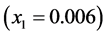 . This happens because of several factors:
the catchability of this genotype is high
. This happens because of several factors:
the catchability of this genotype is high
 and population rates for the genotypes of type
 ,
,
![]() and
and
 (same expected phenotype
 ) are low. The population size rate for the
genotype of type
) are low. The population size rate for the
genotype of type
 with high catchability parameter
 stabilizes at the point around
 . The organisms with genotypes
 and
and
![]() have the highest population rates (around
have the highest population rates (around![]() ).
).
3.2. Example 2. (a)
 and
and
 Are the Greatest
Setting
 greater than the other
 values models epistasis by giving the genotype
 (expected phenotype
 ) a higher prey-induced death rate than the
other organisms with phenotype
) a higher prey-induced death rate than the
other organisms with phenotype . Using these parameters, stabilization took
nearly twice as long as in the previous model. Refer to
Figure 11 and Figure 12.
. Using these parameters, stabilization took
nearly twice as long as in the previous model. Refer to
Figure 11 and Figure 12.
The high value of the catchability parameter
 forces the organism of genotype
 to very small levels, faster than in the previous example. The population size rate
for the organisms of type
to very small levels, faster than in the previous example. The population size rate
for the organisms of type
 with catchability parameter
 is smaller too (around
![]() ). On the other hand, the organisms with lower catchability
values (genotypes
). On the other hand, the organisms with lower catchability
values (genotypes ,
,
 ,
,
![]() , and
, and ) have the highest population densities.
Since
 and mating between the organism of type
 produces all the other genotypes,

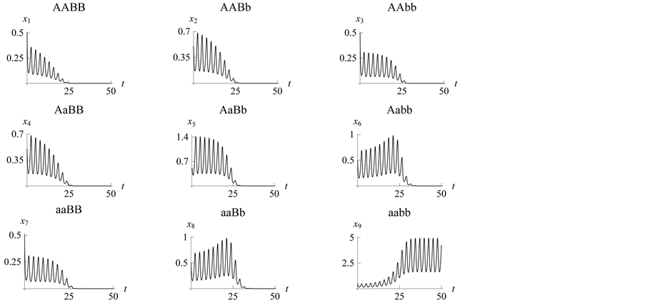
Figure 8. Limit cycles
with![]() ,
,
 and
and![]() . The organism of genotype
. The organism of genotype
![]() survives; the
survives; the
 and
and
![]() alleles go to fixation.
alleles go to fixation.
Figure 9. Stabilization
with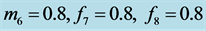
 .
.
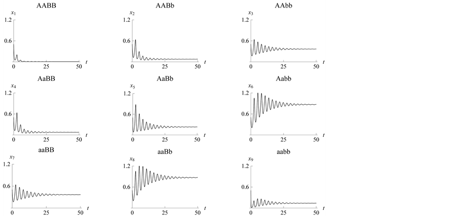
Figure 10. Stabilization
with

 .
.
Figure 11. Stabilization
with

 .
.
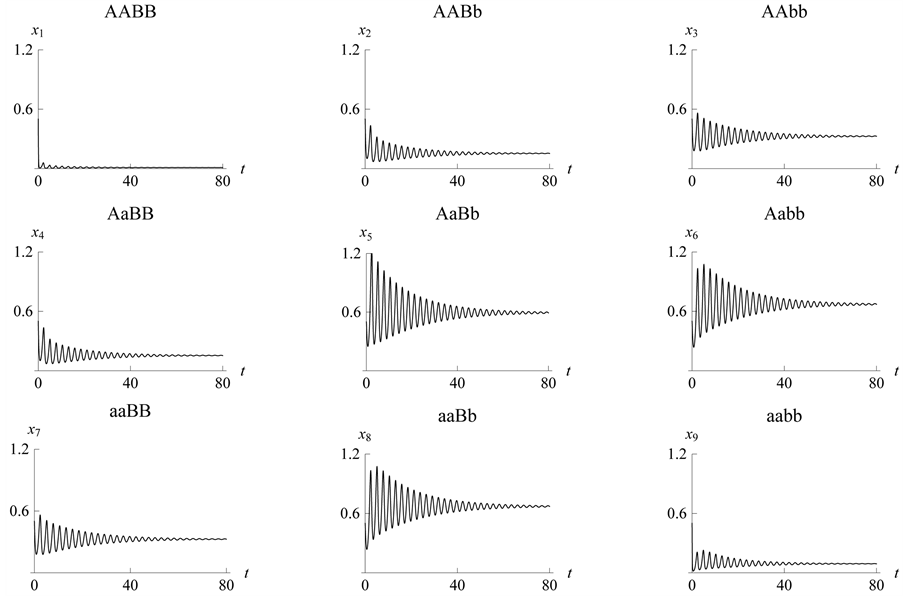
Figure 12. Stabilization
with .
.
and
 (expected phenotype is
 and
and
![]() respectively) have the highest rates and more chances for survival.
respectively) have the highest rates and more chances for survival.
3.3. Example 2. (b)
 and
and
 Are the Greatest While All Other Parameter Values Are 1
This case is interesting by the “slowness” in the rate at which the system stabilizes when compared to the previous two examples. From Figure 13 we see that both populations need around 170 steps to stabilize at one point.
This example numerically indicates that all genotypes except
 and
and
 find stabilization at the hight value population rate point. Both types
 with dominant alleles and the weakest genotype
 with recessive alleles have high catchability value
 and stabilize at the point close to zero (that is, they are close to extinction)
(Figure 14).
and stabilize at the point close to zero (that is, they are close to extinction)
(Figure 14).
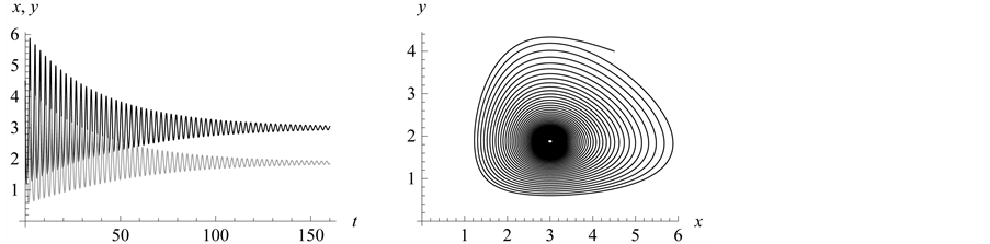
Figure 13. Stabilization
with .
.
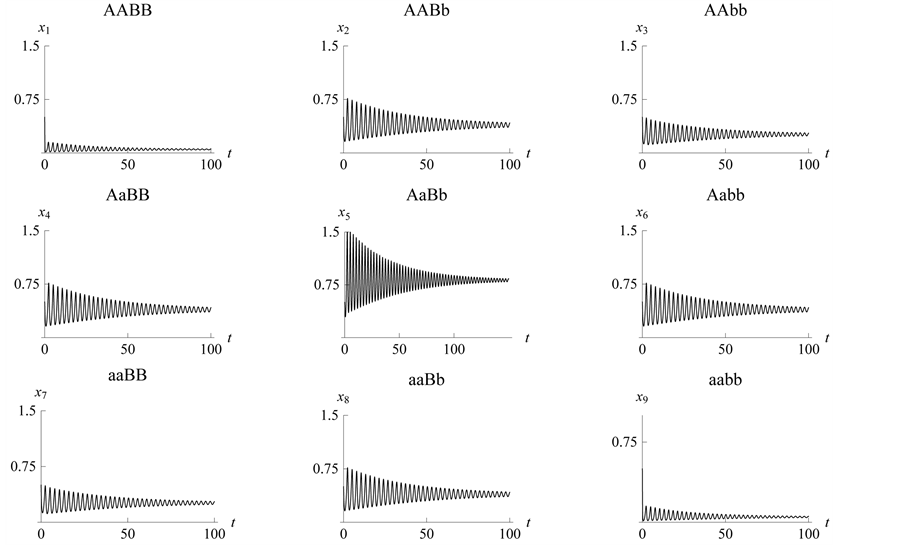
Figure 14. Stabilization
with .
.
3.4. Example 3.
 Is the Smallest: The Catchability of the Organism with Genotype
![]() Is the Lowest
Is the Lowest
Setting
 smaller than the other
 values models epistasis by giving the genotype
 (expected phenotype
 ) a lower prey-induced death rate than the other
organisms with phenotype
) a lower prey-induced death rate than the other
organisms with phenotype . Figure 15
illustrates that the population/density rate of the prey changes from approximately
. Figure 15
illustrates that the population/density rate of the prey changes from approximately
![]() to
to
![]() while the predator population/density rate changes from approximately
while the predator population/density rate changes from approximately
 to
to .
.
Setting
 smaller than the other
 values models epistasis by giving the genotype
 (expected phenotype
 ) a lower prey-induced death rate than the other
organisms with phenotype
) a lower prey-induced death rate than the other
organisms with phenotype . The example illustrates an interesting situation.
The small catchability rate of the species with genotype
. The example illustrates an interesting situation.
The small catchability rate of the species with genotype
 with dominant alleles
 and
and
 and the same catchability rates for the other species with genotypes
 survive the competition between the other genotypes and forces them to extinction.
A critical point around
survive the competition between the other genotypes and forces them to extinction.
A critical point around
![]() can be observed. In this case, the
can be observed. In this case, the
 and
and
 alleles go to fixation (Figure 16 and Figure 17).
3.5. Example 4.
 Is the Smallest;
 Is the Greatest
Both predator and prey populations stabilize at almost the same rate (around
![]() for the predator and
for the predator and
![]() for the prey with the parameter values we use) as shown in
Figure 18.
for the prey with the parameter values we use) as shown in
Figure 18.
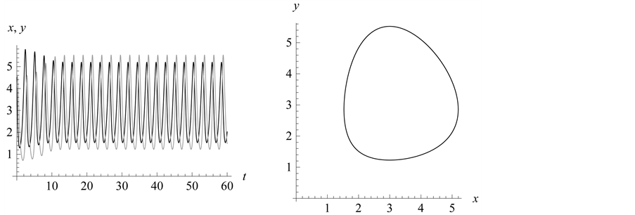
Figure 15. Limit cycle
with . The
. The
 and
and
 alleles go to fixation so the genotype
 is the only one to survive.
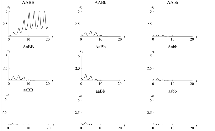
Figure 16. Limit cycle
with . The
. The
 and
and
 alleles go to fixation to the genotype
 is the only one to survive.
When the growth advantage is given to the
![]() organism (with genotype
organism (with genotype ) and because random mating of the organism with
genotype
) and because random mating of the organism with
genotype
 produces all of other genotypes, we observe the stabilization shown in Figure 19. Since
 , all other genotypes stabilize as well.
3.6. Example 5. (a)
 Is the Largest; All Other Parameter Values Are Equal
With these parameter values, the example, which is graphically illustrated in Figure 19, illustrates how the
 - phenotype group (
 ,
,
![]() ,
,
![]() , and
, and![]() ) can be the strongest (or survive with the highest
population/density) with respect to the population sizes/densities of the other
genotypes. In this case, the
) can be the strongest (or survive with the highest
population/density) with respect to the population sizes/densities of the other
genotypes. In this case, the
 and
and
 alleles go to fixation.
Making the weakest species with genotype
 (because the genes
 and
and
 are recessive) more catchable by choosing large catchability parameter values forces
the genotype to extinction. We have also observed
are recessive) more catchable by choosing large catchability parameter values forces
the genotype to extinction. We have also observed
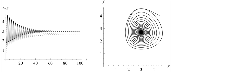
Figure 17.
Stabilization with

 .
.
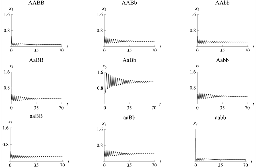
Figure 18.
Stabilization with .
.

Figure 19.
Limit ycle with .
.
that a limit cycle sometimes occurs. Population sizes/densities of the species with
genotypes
 and
and
![]() decrease extremely slowly with the selected parameter values as shown in Figure 20.
decrease extremely slowly with the selected parameter values as shown in Figure 20.
3.7. Example 5. (b) Parameter Value
 Is the Greatest and We Choose the Parameter Values
 and
and
 to Be Smaller
As in the previous example (refer to Figure 17
and Figure 18), high population size/density of
the organism with genotype
 forces the system to stabilize. In this case, the organisms with genotypes
 ,
,
 and
and
 have the highest values because their catchability parameters are the lowest with
respect to the other population sizes/densities of the species with the other genotypes.
The lowest population sizes/densities, as we have seen in the simulation, are the
organisms with genotypes
have the highest values because their catchability parameters are the lowest with
respect to the other population sizes/densities of the species with the other genotypes.
The lowest population sizes/densities, as we have seen in the simulation, are the
organisms with genotypes
 and
and
 (both around
![]() ) (Figure 21 and
Figure 22).
) (Figure 21 and
Figure 22).
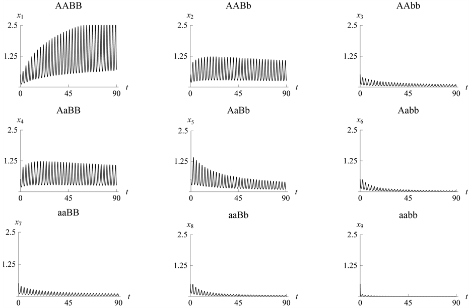
Figure 20. Limit cycle
with .
.
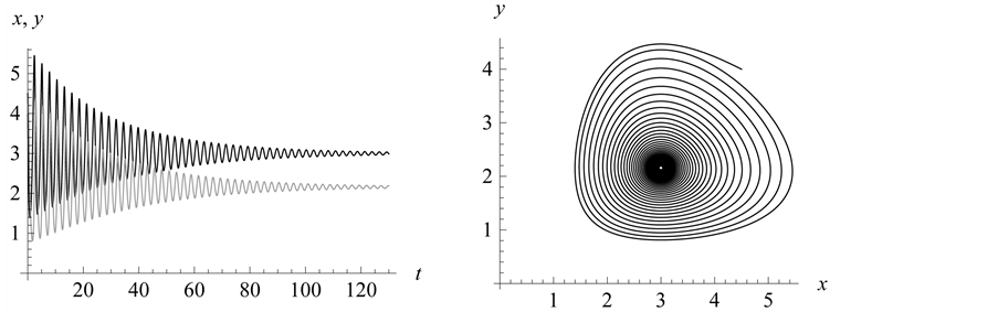
Figure 21. Stabilization
with .
.
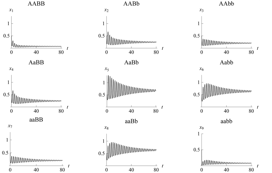
Figure 22. Stabilization
with .
.
4. Conclusions
In this paper we have discussed different cases of epistasis of the prey in a two-locus, two-allele problem in a basic predator-prey relationship. After discussing the most famous example of epistasis in humans, The Bombay Phenotype, we constructed the main model for a two-locus, two-allele problem with nine genotypes. Then we used different values for “catchability” parameters to examine both population sizes as well as genotypic and phenotypic population/densities.
In our simulations and examples, we saw that in different situations limit cycles
or stabilization can occur. The simulations showed that the model was highly sensitive
to the different parameters. Some cases illustrated total extinction of the weakest
types of the prey, while in other examples all population types survived and a limit
cycle occurred. Some interesting examples were observed where the weakest or the
strongest types also became extinct. Since random mating of the organism of type
 produces all of the other genotypes (and phenotypes), this type had the highest
population rate most of the time.
produces all of the other genotypes (and phenotypes), this type had the highest
population rate most of the time.
Future studies might include using different predator-prey models such as epistasis of the predator in a twolocus two-allele problem, epistasis of both predator and prey in the same model, or epistasis in the dangerous predator case. In future studies, we will be able to see how the numerical results obtained here might change or how the situation might evolve differently if epistasis occurs in both the predator and the prey. Other interesting studies would be to incorporate epistasis into competition, cooperation problems, or host-parasite problems.
Computational Remarks
Mathematica 9.0 [9] , was used to create the graphics and perform the computations presented in this paper. Copies of the Mathematica notebooks used are available from the authors by sending a request for them to Jim Braselton at jbraselton@georgiasouthern.edu.
[1] Karlin, S. (1972) Some Mathematical Models of Population Genetics. American Mathematical Monthly, 79, 699-739. http://dx.doi.org/10.2307/2316262
[2] Dean, L. (2005) Blood Groups and Red Cell Antigens. National Center for Biotechnology Information.
[3] Lotka, A.J. (1956) Elements of Mathematical Biology. Dover, New York
[4] Abell, M. and Braselton, J. (2010) Introductory Differential Equations with Boundary Value Problems. 3rd Edition, Academic Press, Boston.
[5] Beltrami, E. (2013) Mathematical Models for Society and Biology. 2nd Edition, Academic Press, Boston.
[6] Murray, J. (2007) Mathematical Biology: I. An Introduction. 3rd Edition, Springer, New York.
[7] Braselton, J., Abell, M. and Braselton, L. (2005) Selective Mating in a Continuous Model of Epistasis. Applied Mathematics and Computation, 171, 225-241. http://dx.doi.org/10.1016/j.amc.2005.01.059
[8] Szathmáry, E. (1993) A Note on the Reduction of the Dynamics of Multilocus Diploid Genetic Systems with Multiplicative Fitness. Journal of Theoretical Biology, 164, 351-358. http://dx.doi.org/10.1006/jtbi.1993.1159
[9] Wolfram Research, Inc. (2013) Dominance, Population Size, and Delayed Inheritance. Evolution, 67, 2011-2023.
Appendix: Ratios of Offspring for Mating Combinations
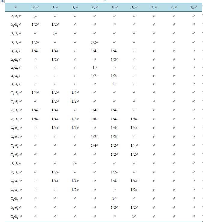
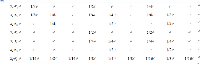
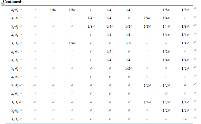
Table A1. Ratios of offspring for
 mating combinations.
NOTES

*Corresponding author.