

Journal of High Energy Physics, Gravitation and Cosmology
Vol.02 No.02(2016), Article ID:65462,23 pages
10.4236/jhepgc.2016.22018
Open Question: Could a Causal Discontinuity Explain Fluctuations in the CMBR Radiation Spectrum?
Andrew Walcott Beckwith
Physics Department, College of Physics, Chongqing University, Chongqing, China

Copyright © 2016 by authors and Scientific Research Publishing Inc.
This work is licensed under the Creative Commons Attribution International License (CC BY).
http://creativecommons.org/licenses/by/4.0/



Received 24 November 2016; accepted 10 April 2016; published 13 April 2016
ABSTRACT
Could a causal discontinuity lead to an explanation of fluctuations in the CMBR radiation spectrum? Is this argument valid if there is some third choice of set structure (for instance do self-referential sets fall into one category or another)? The answer to this question may lie in (entangled) vortex structure of space time, along the lines of structure similar to that generate in the laboratory by Ruutu. Self-referential sets may be part of the generated vortex structure, and we will endeavor to find if this can be experimentally investigated. If the causal set argument and its violation via this procedure holds, we have the view that what we see a space time “drum” effect with the causal discontinuity forming the head of a “drum” for a region of about 1010 bits of “information” before our present universe up to the instant of the big bang itself for a time region less than  seconds in duration, with a region of increasing bits of “information” going up to 10120 due to vortex filament condensed matter style forming through a symmetry breaking phase transition. We address the issue of what this has to do with Bicep 2, the question of scalar-tensor gravity versus general relativity, how to avoid the detection of dust generated Gravity wave signals as what ruined the Bicep 2 experiment and some issues information flow and causal structure has for our CMBR data as seen in an overall summary of these issues in Appendix X, of this document. Appendix XI mentions how to differentiate between scalar-tensor gravity, and general relativity whereas Appendix XII, discusses how to avoid the Bicep 2 mistake again. While Appendix VIII gives us a simple data for a graviton power burst which we find instructive. We stress again, the importance of obtaining clean data sets so as to help us in the eventual detection of gravitational waves which we regard as decisively important and which we think by 2025 or so which will be an important test to discriminate in a full experimental sense the choice of general relativity and other gravity theories, for the evolution of cosmology. Finally, Appendix VII brings up a model for production for gravitons, which is extremely simple. Based upon a formula given in a reference, by Weinberg, in 1971, we chose it due to its illustrative convenience and ties in with Bosonic particles.
Keywords:
Scalar-Tensor Gravity, Bicep 2, CMBR, Causal Structure, Causal Discontinuity

1. Introduction
We start, as stated earlier, by appealing to work done by Ruutu [1] as far as vortex structure, being generated in a laboratory. From here, we ask if there is a possibility of obtaining the same sort of structure in early space-time physics. We will ask, also a question if this vortex filament generates chaos, in the beginning it can have been created by a causal discontinuity in the heart of space-time.
The causal discontinuity condition is in [2] and is integral to the evolution of space time physics. The relevance of this question as presented in the abstract has with CMBR is two-fold. Conventional fluctuations lead to the CMBR angular separation of the particle-horizon distance of about , and this is in line with acoustic peaks in the WMAP power spectrum starting at about
 for the multipole moment. Conventional treatment of the CMBR data makes generous use of error bars. Shankar has raised the specific possibility in his talk “Cosmology beyond the Standard Model” in ICGC-07, Pune, India, and also in print [3] that there is another explanation as to the error bars, namely that as reported in Sarkar’s BadHonnef 07 talk [4] that there is a fluctuation in early universe structure, beyond the normal perturbations associated with the standard model which need to be investigated. In particular, J.J. Blanco-Pillado et al. in 2004 [5] investigated race track models of inflation where there was investigation of a more complex version of a scalar field evolution equation of the form
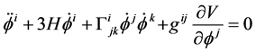 (1)
This has real and imaginary components to the scalar field which can be identified as of the form  for the real part to the scalar field
 , and
 for the imaginary part of the scalar field
 , as well as having
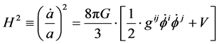 (2)
J.J. Blainco-Pillado et al. [5] use this methodology, using the physics of the Christoffel symbol as usually given by
 (3)
If one has no coupling of terms as in an expanding universe metric of the form [6]
 (4)
Then the Christoffel symbols take the form given by
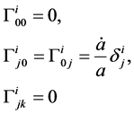 (5)
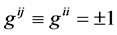
The implications for the scalar evolution equation are that we have
 (6)
If we can write as follows, i.e. say that we have , as well as have
 ,
 (7)
 (8)
 (9)
On the other hand,
 Provided
 (10)
Otherwise, taking into account the causal discontinuity expression, we claim that we will be working with
 provided
 (11)
For very short time duration, and looking at the case for chaotic inflation, we would be working with, in this situation . Set an ansatz with regards to
 provided
 (12)
If , Equation (62)
 (12a)
This would lead to, if provided , and for a short period of time, H is a constant
 (13)
Similarly, for , assuming for a short period of time that H is approximately a constant.
 (14)
Upshot is that for , there is a greater rate of growth in the
 scalar field than is the case when

2. How to Tie in the Entropy with the Growth of the Scale Function?
Racetrack models of inflation, assuming far more detail than what is given in this simplistic treatment provide a power spectrum for the scalar field given by
 (15)
This is assuming a slow roll parameter treatment with , and for
 . Equation (15) would be growing fairly rapidly in line with what is said about Equation (14) above. An increase in scalar power, is then proportional to an increase in entropy via
 (16)
Now, how does this tie in with the lumpiness seen in the CMBR spectra? In an e mail communication, Sarkar summarized the situation up as follows [7] :
“Quasi-DeSitter space-time during inflation has no ‘lumpiness’―it is necessarily very smooth. Nevertheless one can generate structure in the spectrum of quantum fluctuations originating from inflation by disturbing the slow-roll of the inflaton―in our model this happens because other fields to which the inflation couples through gravity undergo symmetry breaking phase transitions as the universe cools during inflation”.
If we use what is in Appendix I, namely the non flat space generalization of the flat space De Alembertian leading to, for a quartic potential as given in Appendix I
 (17)
 (18)
The mass being referred to fades out if there is a temperature increase. So happens that there is one. And this due to the worm hole transfer of thermal heat and the like from a prior universe. This is done and can be made far more complex if the De Alembertian has off diagonal terms in it
i.e. if one does not insist upon simple Euclidian space, the Laplacian takes the form [6]
 (19)
We claim that the generalization for Equation (17) and Equation (18) will lead in the case of cooling for a scalar field system in the aftermath of immediate rapid expansion of the scalar field a very different, and far more complicated dynamic than is given by Equation (18)
Recall what is given in modeling the pure Dilatonic potential, i.e. as given by Lalak, Ross, and Sakar [3] (2006). This potential has a minimum if B/A > 1 where it can vanish, and it has a non zero minimum if we set 
 (20)
This is assuming that we are having , leading to minima for
 , with k being the positive and negative integers, i.e. this helps delineate between two condensates. If we have a complex scalar field
 . We have moduli arguments which add far more structure, i.e. we are getting into Calabi-Yau compactification issues. Appendix II offers a simpler potential system. But that system plus Equation (20) must have spectral index behavior, i.e. reflecting inflation and the early universe, which matches WMAP data.
Point which is to be made here, is that the richer the structure with respect to Equation (20), and its race track version which has real and imaginary components to a scalar field, the less tenable the simple Equation (17) pictures of simply rising and falling scalar potentials are. So the following claim is made.
CLAIM 1: In the initial phase of expansion in an inflationary sense, the period of time  corresponds with a scalar field given by Equation (17) and Equation (18). As we have a rapidly increasing temperature, we have no complexity of the sort implied by Equation (20) above.
CLAIM 2: In the cool down period before the re heating period after inflation, we have additional structure put in, enough so, so that multiple minima and fluctuations exist which would give far more definition as to local scalar power spectra. I.e. we are looking at
 (21)
Provided that we have a nonzero minimum if we set  for
 , we claim that then we are having the basis for non zero fluctuations seen as given in Sarkar’s Bad Honnef 07 portrayal of CMBR [7] .
We can use the criteria of Appendix III, which gives realistic data input parameters as to the variance of the CMBR spectra. In particular, we can take Equation (3) of Appendix III and splicing that in on a new derivation as to  power spectra. I.e.
 of Appendix IV is an incredibly crude model, which depends upon Equation (3) of that section for a power law, which then leads to how to re construct, assuming NO time dependence upon the Hubble Parameter ; i.e.
 , to come up with a tensor type of expression for
 based upon what can be called very naïve assumptions.
Here we can make the following assertion. Especially with regards to Gravitational waves. This is from Durrer [8] , and is a foundation for additional work which can be done
i.e.
 (22)
We can appeal to simplified models as to how to come up with . First of all, consider the causal discontinuity equation argument. This is one phase as to implementation, i.e. look at
 . This is where we
are working directly with Equation (12) in part, and at the regime of at least partial causal discontinuity [2] , we are working with Equation (1). The interplay between these two equations in part can lead to an effective re construction of a potential system, which in part should in its structure, have some similarities with the race track potential. Appendix V also gives guidance as to re construction of the potential system we can work with, and also compare it with the different race track models so outlined.
In addition to this treatment of how to get a CMBR reconstruction of gravitational tensor fluctuations, we can also look at observational efforts to confirm, or falsify different models of , i.e. how the
entropy varies will be in its own way will affect the power spectra, which in turn affects confirming or falsify-
ing the spectral index . Here, N is the number of e folding in inflation and we can
follow through on elementary calculations of how P varies due to choices of potential system we are examining. I.e. recall Sarkar’s 2001 investigation of a simple choice of variant of the standard chaotic inflationary potential given by [9]
 (23)
Sarkar treated the inflaton as having a varying effective mass, with an initial value of effective mass of  given a before and after phase transition value of
 (24)
This is, when Sarkar did it, with  as a coupling term. This would also affect the spectral in-
dex value, and it also would be a way to consider an increase in inflation based entropy. The only drawback to this phenomenological treatment is that it in itself does not address the formation of an instanton in the very beginning of inflation, a serious draw back since this does not also give an entry into the formation of the layers of complexity which we think is more accurately reflected in the transferal of state from a growing value of the magnitude of the scalar field as given by Equation (17) and Equation (18) as temperature flux flows in from a prior universe, to the cooling off period we think is necessary for the formation of a complex scalar field and its analogies in the race track style models, as in Equation (20), and Appendix I below. Equation (72) with its treatment of tensorial contributions to the CMBR has its counterpart, an implied release in relic gravitons which may, or may not be amendable to observational techniques. We would most likely imply their existence indirectly via use of Equation (22) and seeing if they can be linked to the behavior of the inflation generating a new burst of entropy at the onset of inflation. Appendix VI shows what we may wish to consider as to relic graviton production which is linkable to the worm hole, and causal discontinuity discussion we have brought up, with regards to early universe entropy generation. We also will make reference that this has been linked to brane theory via Appendix VII material.
3. Conclusion: Match up with Smoot’s Table
In a colloquium presentation done by Dr. Smoot in Paris [10] (2007), he alluded to the following information theory constructions which bear consideration as to how much was transferred between a prior to the present universe in terms of information “bits”.
1) Physically observable bits of information possibly in present Universe-0180.
2) Holographic principle allowed states in the evolution/development of the Universe-10120.
3) Initially available states given to us to work with at the onset of the inflationary era-1010.
4) Observable bits of information present due to quantum/statistical fluctuations-108.
Our guess is as follows. The thermal flux so implied by the existence of a worm hole accounts for perhaps 1010 bits of information. These could be transferred via a worm hole solution from a prior universe to our present, and that there could be, perhaps 10120 minus 1010 bytes of information temporarily suppressed during the initial bozonification phase of matter right at the onset of the big bang itself.
Then after the degrees of freedom dramatically drops during the beginning of the descent of temperature from about  to at least three orders of magnitude less, we move out from an initial red shift
 .
To [11]
 (25)
Whichever model we can come up with that does this is the one we need to follow, experimentally. And it gives us hope in confirming if or not we can eventually analyze the growth of structure in the initial phases of quantum nucleation of emergent space time [12] . We also need to consider the datum so referenced as to the irregularities as to the cooling down phase of inflation, as mentioned by Sakar [7] .
The race track models, after the inflation begins to decline will be ideal in getting the couplings, and the symmetry breaking. We will refer to this topic in a future publication. We can make a few observations though about the coupling so assumed. First, there is a question of if or not there is a finite or infinite fifth dimension. String theorists have argued for a brane-world with a warped, infinite extra dimension allowing for the inflation to decay into the bulk so that after inflation, the effective dark energy disappears from our brane. This is achieved by shifting away the decay products into the infinity of the 5th dimension [13] . Nice hypothesis, but it presumes CMB density perturbations, has their origin in the decay of MSSM predicted particles. It will reduce the dynamics of the inflation to be separation between a  brane and
 anti-brane via a moduli argument.
What if we do not have an infinite fifth dimension? What if it is compactified only? We then have to change our analysis.
Another thing. We place limits on inflationary models; for example, a minimally coupled  is disfavored at more than 3 σ. Result? Forget quartic inflationary fields, as has been show by Peiris, Hingshaw et al. [14] . We can realistically hope that WMAP will be able to parse through the race track models to distinguish between the different candidates. So far “First-Year Wilkinson Microwave Anisotropy Probe (WMAP) 1 Observations: Implications for Inflation” is giving chaotic inflation a run for its money. We shall endeavor for numerical work using some of the tools brought up in this present discussion for falsifying or confirming in Figure 1 and Figure 2 of this text which show variance in the CMBR spectrum. Appendix VII is a simple model for relic Graviton production. Appendix VIII suggests data for a relic graviton burst. In addition, Appendix X addresses the

Figure 1. As given by Sarkar, from his web site. Copied from Dr. Sarkar’s Bad Honnif 07 talk and re produced here with explicit permission of the original presenter. Shows the glitches which need to be addressed in order to make a CMBR data set congruent with an extension of the standard model of cosmology.

Figure 2. Sakar figure about CMBR, from Bad Honnif.
matter of information flow, in terms of details on information theory and the like and also Dowker causal structure, and how it may tie into the subject of our inquiry as stated in the title and abstract. Appendix X is a re statement of the basic summary points of this paper with regards to causal structure and discontinuity and re iterates what is scattered through this document for a quick read. Appendix XI addresses the issue of what may relate this to the question of if Scalar-tensor gravity is favored, or General relativity, and Appendix XII discusses the tie in with differentiating our inquiry from problems which destroyed the fidelity of Bicep 2’s measurements, due to dust generated GW signals which is what we wish to avoid at all costs in this inquiry. Our conclusion is that we need, especially, to consider fully the issues raised in Appendix X, which will then allow us, to if we are careful to distinguish between scalar-tensor gravity in Appendix XI, and GR as a foundational construction in cosmology. Clean data sets, and observational platforms as brought up in Appendix XII, will commence, if done rigorously, to enhance the probability of relic GW being measured instead of the chaos multi source generation of gravitational waves, created by dust. Note Appendix X, has 2 sub sessions and they are meant to be a focus of this document upon the information flow aspect of this paper. The entire document Appendix X is meant to summarize the theme of information flow and causal discontinuity as it may affect the CMBR in this very long document. For convenience.
Acknowledgements
This work is supported in part by National Nature Science Foundation of China grant No. 11375279.
Cite this paper
Andrew Walcott Beckwith, (2016) Open Question: Could a Causal Discontinuity Explain Fluctuations in the CMBR Radiation Spectrum?. Journal of High Energy Physics, Gravitation and Cosmology,02,186-208. doi: 10.4236/jhepgc.2016.22018
References
- 1. Ruutu, V., Eltsov, V, Gill, A., Kibble, T., Krusius, M., Makhlin, Y.G., Placais, B., Volvik, G. and Wen, Z. (1996) Vortex Formation in Neutron-Irradiated 3He as an Analog of Cosmological Defect Formation. Nature, 382, 334-336.
- 2. Beckwith, A., Li, F.Y., Yang, N., Dickau, J., Stephenson, G. and Glinka, L. (2011) Is Octonionic Quantum Gravity Relevant Near the Planck Scale? If Gravity Waves Are Generated by Changes in the Geometry of the Early Universe, How Can We Measure Them? Relativity and Cosmology. http://vixra.org/abs/1101.0017
- 3. Lalak, Z., Ross, G. and Sakar, S. (2007) Racetrack Inflation and Assisted Moduli Stabilization. Nuclear Physics B, 766, 1-20.
- 4. http://www-thphys.physics.ox.ac.uk/user/SubirSarkar/
- 5. Blanco-Pillado, J., Burgess, C., Cline, J., Escoda, C., Gomez-Reino, M., Kallosh, R., Line, A. and Quevedo, F. (2004) Racetrack Inflation. Journal of High Energy Physics, 2004, 23 p.
- 6. Carroll, S. (2005) Spacetime and Geometry: An Introduction to General Relativity. Addison Wesley Co., San Francisco.
- 7. Private Communications with Subir Sarkar. Received as of January 2008.
- 8. Durrer, R. (2004) Cosmological Perturbation Theory. In: Papantonopoulos, E., Ed., Physics of the Early Universe, Lecture Notes in Physics, Vol. 653, Springer-Verlag, Berlin.
- 9. Hunt, P. and Sakar, S. (2004) Multiple Inflation and the WMAP “Glitches”. Physical Review D, 70, Article ID: 103518.
- 10. Smoot, G. (2007) CMB Observations and the Standard Model of the Universe. 11th Paris Cosmology Colloquium, 18 August 2007. http://chalonge.obspm.fr/Programme2007.html
- 11. Sanchez, N. (2007) Understanding Inflation and the Dark Energy in the Standard Model of the Universe. 11th Paris Cosmology Colloquium, 18 August 2007. http://chalonge.obspm.fr/Programme2007.html
- 12. Enqvist, K., Mazumdar, A. and Perez-Lorenzana, A. (2004) Dumping Inflaton Energy out of This World. Physical Review D, 70, Article ID: 103508
- 13. Peiris, H.V., Komatsu, E., Verde, L., Spergel, D., Bennett, C., Halpern, M., Hinshaw, G., Jarosik, N., Kogut, A., Limon, M., Meyer, S., Page, L., Tucker, G., Wollack, E. and Wright, E. (2003) First-Year Wilkinson Microwave Anisotropy Probe (WMAP) Observations: Implications For Inflation. The Astrophysical Journal Supplement Series, 148, 213-231.
- 14. Conformal Cyclic Cosmology, Dark Matter, and Black Hole Evaporation. Lecture notes taken at IGC conference, with respect to the Penrose presentation, plus questions asked of the lecturer in the aftermath of that presentation. http://www.gravity.psu.edu/igc/conf_files/program_complete.pdf
- 15. Brax, Ph., Davis, A., Davis, S., Jeannerot, R. and Postman, M. (2008) D-Term Uplifted Racetrack Inflation. Journal of Cosmology and Astroparticle Physics, JCAP01(2008) 08.
- 16. Samtleben, D., Staggs, S. and Winstein, B. (2007) The Cosmic Microwave Background for Pedestrians: A Review for Particle and Nuclear Physicists. Annual Review of Nuclear and Particle Science, 57, 245-283.
- 17. Padmanabhan, T. (2000) Theoretical Astro Physics, Volume 1: Astrophysical Processes. Cambridge University Press, Cambridge.
- 18. Zhitinisky, A. (2003) Dark Matter as Dense Color Superconductor. Nuclear Physics B-Proceedings Supplements, 124, 99-102.
- 19. Rothman, T. and Boughn, S. (2006) Can Gravitons Be Detected? Foundations of Physics, 36, 1801-1825.
- 20. Beckwith, A.W. (2007) How Can Brane World Physics Influences the Formation of a Cosmological Constant Relevant to Graviton Production? E.J.T.P., 4, 105-142. http://arxiv.org/abs/physics/0612010
- 21. Park, D.K., Kim, H. and Tamarayan, S. (2002) Nonvanishing Cosmological Constant of Flat Universe in Brane-World Scenario. Physics Letters B, 535, 5-10.
- 22. Barvinsky, A.O. and Kamenschick, A.Yu. (2006) Thermodynamics from Nothing: Limiting the Cosmological Constant Landscape. Physical Review D, 74, Article ID: 121502.
- 23. Guth, A.H. (1981) Inflationary Universe: A Possible Solution to the Horizon and Flatness Problems. Physical Review D, 23, 347-356.
- 24. Guth, A.H. (2000) Inflation and Eternal Inflation. http://www.citebase.org/cgi-bin/citations?id=oai:arXiv.org:astro-ph/0002156
- 25. Guth, A.H. (2003) Eternal Inflation. http://online.itp.ucsb.edu/online/strings_c03/guth/pdf/KITPGuth_2.pdf
- 26. Weinberg, S. (1972) Gravitation and Cosmology: Principles and Applications of the General theory of Relativity. John Wiley & Sons, Inc., New York.
- 27. Fontana, G. (2005)Gravitational Wave Propulsion. In: El-Genk, M.S., Ed., CP746, Space Technology and Applications International Forum-STAIF, American Institute of Physics, Melville.
- 28. Park, D. (1955) Radiations from a Spinning Rod. Physical Review, 99, 1324-1325.
- 29. Beckwith, A.W. (2006) Does a Randall-Sundrum Brane World Effective Potential Influence Axion Walls Helping to Form a Cosmological Constant Affecting Inflation? AIP Conference Proceedings, 880, 1170-1180. http://www.citebase.org/cgi-bin/citations?id=oai:arXiv.org:gr-qc/0603021
- 30. Leach, J.A. and Lesame, W.M. (2005) Conditional Escape of Gravitons from the Brane. arXiv:gr-qc/0502109
- 31. Dalarsson, M. and Dalarsson, N. (2005) Tensors, Relativity and Cosmology. Elsevier Academic Press, Burlington.
- 32. Crowell, L. (2005) Quantum Fluctuations of Space Time. In: World Scientific Series in Contemporary Chemical Physics, Vol. 25, Singapore.
- 33. Beckwith, A.W. (2007) Symmetries in Evolving Space Time from Present to Prior Universes. arXiv:math-ph/0501028
- 34. Frampton, P. and Baum, L. (2007) Turnaround in Cyclic Cosmology. Physical Review Letters, 98, Article ID: 071301.
- 35. Dowker, F. (2005) Causal Sets and the Deep Structure of Space-Time. In: Akshtekar, A., Ed., 100 Years of Relativity, Space-Time Structure: Einstein and Beyond, World Press Scientific, Singapore, 445-464.
- 36. Lloyd, S. (2002) Computational Capacity of the Universe. Physical Review Letters, 88, Article ID: 237901.
- 37. Beckwith, A. (2016) Gedanken Experiment Examining How Kinetic Energy Would Dominate Potential Energy, in Pre-Planckian Space-Time Physics, and Allow Us to Avoid the BICEP 2 Mistake. Journal of High Energy Physics, Gravitation and Cosmology, 2, 75-82. http://dx.doi.org/10.4236/jhepgc.2016.21008
- 38. Corda, C. (2009) Interferometric Detection of Gravitational Waves: The Definitive Test for General Relativity. International Journal of Modern Physics D, 18, 2275-2282. http://arxiv.org/abs/0905.2502
- 39. Das, S., Mukherje, S. and Souradeep, T. (2015) Revised Cosmological Parameters after BICEP 2 and BOSS. JCAP, 02 (2015) 016. http://arxiv.org/abs/1406.0857
- 40. Van Den Broeck, C., et al. (2015) Gravitational Wave Searches with Advanced LIGO and Advanced Virgo. http://arxiv.org/pdf/1505.04621v1.pdf
- 41. Cowen, R. (2015) Gravitational Waves Discovery Now Officially Dead: Combined Data from South Pole Experiment BICEP2 and Planck Probe Point to Galactic Dust as Confounding Signal. http://www.nature.com/news/gravitational-waves-discovery-now-officially-dead-1.16830
- 42. Cowen, R. (2014) Full-Galaxy Dust Map Muddles Search for Gravitational Waves. http://www.nature.com/news/full-galaxy-dust-map-muddles-search-for-gravitational-waves-1.15975
- 43. Beckwith, A. (2016) Gedanken Experiment for Degree of Flatness, or Lack of, in Early Universe Conditions. Journal of High Energy Physics, Gravitation and Cosmology, 2, 57-65. http://dx.doi.org/10.4236/jhepgc.2016.21006
Appendix I. The D’Albembertain Operation in an Equation of Motion for Emergent Scalar Fields
We begin with the D’Albertain operator as part of an equation of motion for an emergent scalar field. We refer to the Penrose potential ( with an initial assumption of Euclidian flat space for computational simplicity) to account for, in a high temperature regime an emergent non zero value for the scalar field  due to a zero effective mass, at high temperatures [14] .
When the mass approaches far lower values, it, a non zero scalar field re appears.
Leading to  as a vanishingly small contribution to cosmological evolution.
Let us now begin to initiate how to model the Penrose quintessence scalar field evolution equation. To begin, look at the flat space version of the evolution equation
 (1)
This is, in the Friedman-Walker metric using the following as a potential system to work with, namely:
 (2)
This is pre supposing , that one is picking a curvature signature which is compatible with an open universe.
That means  as possibilities. So we will look at the
 values. We begin with.
 (3)
We find the following as far as basic phenomenology, namely
 (4)
 (5)
The difference is due to the behavior of . We use
 ~axion mass
 in asymptotic limits with
 (6)
Appendix II. Managing What to Do with Racetrack Inflation, as Cool Down from Initial Expansion Commences
P. Brax, A. Davis et al. [15] devised a way to describe racetrack inflation as a way to look at how super gravity directly simplifies implementing how one can have inflation with only three T (scalar) fields. The benefit to what we work with is that we may obtain two gaugino condensates and look at inflation with a potential given by [15]
 (1)
This has scalar fields  as relatively constant and we can look at an effective kinetic energy term along the lines of
 (2)
This ultra simple version of the race track potential is chosen so that the following conditions may be applied.
1) Exist a minimum at ; i.e. we have
 , and
 , when we are not considering scalar fields
 .
2) We set a cosmological constant equal to zero with .
3) We have a flat saddle at ; i.e.
 .
4) We re-cale the potential via  so as to get the observed power spectra
 .
Doing all this though frequently leads to the odd situation that  must be small so that
 in a race track potential system when we analyze how to fit Equation (1) for flat potential behavior modeling inflation. This assumes that we are working with a spectra index of the form so that if the scalar field power spectrum is
 (3)
Then the spectral index of the inflation is consistent with WMAP data. I.e. if we have the number of e foldings 
 (4)
These sorts of restrictions on the spectral index will start to help us retrieve information as to possible inflation models which may be congruent with at least one layer of WMAP data. This model says nothing about if or not the model starts to fit in the data issues Sarkar identified in is Pune, India lecture in 2007.
Appendix III. Basic Physics of Achieving Minimum Precision in CMBR Power Spectra Measurements
Begin first of all looking at
 (1)
This leads to consider what to do with
 (2)
Samtleben et al. [16] consider then what the experimental variance in this power spectrum, to the tune of an achievable precision given by
 (3)
 is the fraction of the sky covered in the measurement, and
 is a measurement of the total experimental sensitivity of the apparatus used. Also
 is the width of a beam, while we have a minimum value of
 which is one over the fluctuation of the angular extent of the experimental survey.
i.e. Contributions to  uncertainty from sample variance is equal to contributions to
 uncertainty from noise. The end result is
 (4)
Appendix IV. Cosmological Perturbation Theory and Tensor Fluctuations (Gravity Waves)
Durrer [8] reviews how to interpret  in the region where we have
 , roughly in the region of the Sachs-Wolf contributions due to gravity waves. We begin first of all by looking at an initial perturbation, using a scalar field treatment of the “Bardeen potential”
 This can lead us to put up, if
 is the initial value of the Hubble expansion parameter
 (1)
and
 (2)
Here we are interpreting A = amplitude of metric perturbations at horizon scale, and we set , where
 is the conformal time, according to
 = physical time, where we have a as the scale factor.
Then for , and
 , and a pure power law given by
 (3)
We get for tensor fluctuation, i.e. gravity waves, and a scale invariant spectrum with 
 (4)
Appendix V. Formation of the Scalar Field, Bifurcation Results
Start with Padamadans’s formulas [17]
 (1)
 (2)
If  is a constant, Equation (2) gives us zero scalar field values at the beginning of quantum nucleation of a universe. At the point of accelerated expansion (due to the final value of the cosmological constant), it also gives an accelerating value of the cosmological scale-factor expansion rate. We justify this statement by using early-universe expansion models, which have
 . This leads to the derivative of
 going to zero. This is similar to present-time development of the scalar factor along the lines of
 , also leading to the derivative of
 going to zero. When both situations occur, we have the scale factor
 . Between initial and later times, the scale factor no longer has exponential time dependence, due to it growing far more slowly, leading to
 .
Both regimes as specified by Equation (2) above lead to zero values for a quintessence scalar field. But it does not stop there. We will show later that in actuality, the scalar field likely damps out far before the CMBR barrier value of expansion when Z = 1100, about 380,000 to 400,000 years after the big bang.
We show this by noting that in Equation (2), the time derivative of  goes to zero when both the scale factors
 , and
 . The exponential scale factors in both cases (the initial inflationary environment and the present era) lead to the time derivative of the
 expression in Equation (2) going to zero.
Sub point to claim 1: The existence of two zero values of the scalar field  at both the onset and at a later time implies a bifurcation behavior for modeling quintessence scalar fields. This is due to the non-zero
 values right after the initiation of inflation.
Appendix VI. Open Questions as to What the Large Vacuum Energy Implies for Initial Conditions for Graviton Production, plus Graviton Production in a Relic Setting
If we have a non infinite but huge negative value of the cosmological vacuum energy in the wormhole, then we have 1010 bits of computing information. When we leave the wormhole, we have 10120 bits of computing information. We specify a transition between the two regions in terms of a causal discontinuity regime created by a(t) chaotic behavior due initially to the initially very large value of thermal vacuum energy transmitted.
Details, and many more of them are needed to bridge this transition to the problem of structure formation and a drop of temperature. If we look at Ruutu’s [1] (1996) ground breaking experiment we see vortex line filaments rapidly forming. Here are a few open questions which should be asked.
1) Do the filaments in any shape or form have an analogy to the cosmic strings so hypothesized by String theorists? My guess is a flat MAYBE but one cannot be certain of this. This deserves to be analyzed fully. If they have an analogy to cosmic strings, then what is the phase transition from a maximally entangled space time continuum, with a soliton type behavior for temperatures of the order of  to the formation of these stringy structures?
2) What is the mechanism for the actual transition from the initial “soliton” at high temperatures to the symmetry breaking phase transition? This is trickier than people think. Many theorists consider that, in tandem with Ruutu’s [1] (1996) experiment that Axion super partners, Saxions, actually are heated up and decay to release entropy. Do we have structures in initial space time analogous to super fluids allowing us to come up with such a transformation? Do Axions/Saxion super partner pairs exist in the onset of thermal transition from a prior universe to our present universe? How could this be experimentally determined with rigorous falsifiable experimental analysis?
3) One of the models considered as a super fluid candidate for this model has been the di quark one. This however was advanced by Zhitinisky [18] (2002) in terms of “cold dark matter”. Could some analogy to di quarks be used for initial states of matter thermally impacted by a transfer of thermal energy via a wormhole to form a cosmic “bubble” in line with the initial plasma state given in Ruutu’s [1] (1996) experiment?
4) Do the formation of such initial conditions permit us to allow optimal conditions for graviton production? If so, can this be transferred to engineering prototypes? How can this be modeled appropriately?
Here is a very simplified model as to what we may be able to expect if there is actual relic graviton production. I.e. Detecting gravitons as spin 2 objects with available technology. To briefly review what we can say now about standard graviton detection schemes, Rothman [19] states that the Dyson seriously doubts we will be able to detect gravitons via present detector technology. The conundrum is that if one defines the criterion for observing a graviton as
 (1)
Here,
 (2)
This has  a graviton sources luminosity divided by total luminosity and R as the distance from the graviton source, to a detector. Furthermore,
 and
 a constants r, while
 is the graviton P.E. As stated in the manuscript, the problem then becomes determining a cross section
 for a graviton production process and
 .
If this is the case, then what can we do to see how relic gravitons may emerge if we have a worm hole transferred burst of thermal/ vacuum energy? [20] (Table A1).
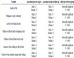
Table A1. With respect to phenomenology.
Also, one can expect a difference in the upper limit of Park’s four dimensional inflation [21] value for high temperatures, on the order of 10 to the 32 Kelvin, and the upper bound, as Barvinsky (2006) [22] predicts. If put into the Hartle-Hawking’s wave function, this difference is equivalent to a nucleation-quantization condition, which, it is claimed, is a way to delineate a solution to the cosmic landscape problem that Guth (1981, 2000, 2003) [23] - [25] discussed. In order to reference this argument, it is useful to note that Barvinsky in (2006) [22] came up with
 (3)
A minimum value of
 (4)
This is in contrast to the nearly infinite value of the Planck’s constant as given by Park (2003) [21] .  is defined by Park (2003).with
 and
 , and
 so that
 (5)
As opposed to a minimum value as given by Park (2003) [21] (Table A2)
 (6)
Appendix VII. The Weinberg Graviton Production Formula for Relic Gravitons
As is well known, a good statement about the number of gravitons per unit volume with frequencies between  and
 may be given by (assuming here, that
 , and K is denoting Kelvin temperatures, where Gravitons have two independent polarization states), as given by Weinberg (1972) [26]
 (1)
The hypothesis presented here is that input thermal energy (given by the prior universe) inputted into an initial cavity/region (dominated by an initially configured low temperature Axion domain wall) would be thermally excited to reach the regime of temperature excitation. This would permit an order-of-magnitude drop of Axion
density  from an initial temperature
 .
Table A2. What can be said about cosmological L in 5 and 4 dimensions.
Appendix VIII. Graviton Power Burst
To do this, one needs to refer to a power spectrum value that can be associated with the emission of a graviton. Fortunately, the literature contains a working expression of power generation for a graviton produced for a rod spinning at a frequency per second , per Fontana [27] (2005), for a rod of length
 and of mass m a formula for graviton production power. This is a variant of a formula given by Park [28] (1955), with mass

 (8)
The contribution of frequency here needs to be understood as a mechanical analogue to the brute mechanics of graviton production. The frequency  is set as an input from an energy value, with graviton production number (in terms of energy) derived via an integration of Equation (7) above
 . This value assumes a huge number of relic gravitons are being produced, due to the temperature variation.
 (9)
And then one can set a normalized “energy input” as ; with
 , which leads to the following table of results, where
 is an initial temperature of the pre-inflationary universe condition [29] (Table 3A).
Here, N1 refers to a net graviton numerical production value as given by Equation (9). There is a distinct power spike of thermal energy that is congruent with a relic graviton burst.
Appendix IX. Using Our Bound to the Cosmological Constant to Link Relic Graviton Production to Branes
We use our bound to the cosmological constant to obtain a conditional escape of gravitons from an early universe brane. To begin, we present using the paper written by Leach et al. on conditions for graviton production [30]
 (1)
Also there exists an “impact parameter”
 (2)
This leads to, practically, a condition of “accessibility” via PP R so defined is with respect to “bulk dimensions”
 (3)
 (4)
Here, k = 0 for flat space, k = −1 for hyperbolic three space, and k = 1 for a three sphere, while an radius of curvature
Table 3A. Graviton burst.
 (5)
Here, we have that we are given
 (6)
Park et al. note that if we have a “horizon” temperature term
 (7)
We can define a quantity
 (8)
Then there exists a relationship between a four-dimensional version of the , which may be defined by noting
 (9)
So
 (10)
In working with these values, one should pay attention to how  is defined by Park, et al. [21]
 (11)
Here, I am defining  as being an input from changes in the actual potential system due to
 (12)
Here we are looking at how the initial vacuum energy ‘cosmological constant’ parameter may be effected by a change in the potential system with the  tern with different temperature values implied for input into the four dimensional vacuum energy. i.e.
 starts off with a given temperature value input as we look at
 for a maximized potential value, and subsequently dropping as the potential system evolves to a different value as inflation proceeds.
This, for potential,  is defined via transition between the first and the second potentials of the form given by
 (13)
Sarkar treated the inflation as having a varying effective mass, with an initial value of effective mass of  given a before and after phase transition value of
 (14)
Either this potential can be used, or we just use a variant of a transition to the race track potential given by
 (15)
This with a version of the scalar field in part be minimized. This is assuming that we are having , leading to minima for
 , with k being the positive and negative integers, i.e. this helps delineate between two condensates. If we have a complex scalar field
 . We have moduli arguments which add far more structure. Either type of structure can be used and put in so we come up with an effective value for a potential system. I.e. at a given
 (16)
Appendix X. Accessing Information Flow and Causal Discontinuity
This paper uses a special metric that is congruent with the Wheeler-De Witt equation, which can be explained as follows. If one rewrites the Friedmann equation using Classical mechanics, we can obtain a Hamiltonian, using typical values of . Where
 can be roughly thought of as the “momentum” of the scale factor a(t), and L is the Lagrangian of our modeled system. The most straightforward presentation of this can be seen
in Dalarsson (2005) [31] . Afterwards, momentum is quantized via , and then with some rewrite initially, one can come up with a time-independent equation looking like
 . Crowell, among others, found a way to introduce a pseudo-time component that changed the
 equation to one that has much
the same flavor as a pseudo-WKB approximation to the Schrodinger equation. This, with some refinements, constitutes what we used for forming a “wormhole” bridge.
We referenced the Reissner-Nordstrom metric. This is a metric that is similar to the space-time metric used for black hole physics, i.e., black holes with a charge. With some modifications, this is the metric that Crowell (2005) [32] used to form his version of the Wheeler-De Witt equation with a wave functional, similar to the WKB equation (i.e. it is still semiclassical), to form the wave functional solution. Crowell (2005) used this solution as a model of a bridge between a prior universe and our own. To show this, one can use results from Crowell (2005) on quantum fluctuations in space-time, which provides a model from a pseudo time component version of the Wheeler De Witt equation, using the Reinssner-Nordstrom metric to help obtain a solution that
passes through a thin shell separating two space-times. The radius of the shell,  separating the two space-
times is of length  in approximate magnitude, leading to a multiplication of the time component for the Reissner-Nordstrom metric: [32]
 (1)
This has:
 (2)
Note that Equation (2) referenced above is a way to link this metric to space-times via the following model of energy density equation, linked to a so called “membrane” model of two universes separated by a small “rescaled distance” . In practical modeling,
 is usually of the order of magnitude of the smallest possible unit of space-time, the Planck distance,
 , as a quantum approximation put into general relativity. The equation linking Equation (2) to energy density
 is of the form:
 (3)
Frequently, this is simplified with the term, . In addition, following temperature dependence of this parameter, as outlined by Park (2003) leads to
 (4)
This is a wave functional solution to a Wheeler De Witt equation bridging two space-times. The solution bridging two space-times is similar to one made by Crowell (2005) [32] between these two space-times with “instantaneous” transfer of thermal heat
 (5)
This equation has  as a cyclic and evolving function of frequency, time, and spatial function, also applicable to
 with
 .
It is asserted here that a thermal bridge in wormhole form exists as a bridge between a prior and present universe. Furthermore, it is asserted that the existence of this bridge is part of a necessary condition for thermal energy transfer between a prior and present universe. The prior universe shrinks to a singularity at the time that thermal energy is transferred to our present universe, thereby helping to initiate cosmological inflation. dominated. This is due in part to the absolute value of the five-dimensional “vacuum state” parameter varying with temperature T, as Beckwith (2007) [33] writes:
 (6)
This contrasts with the more traditional four-dimensional version of the same, without the minus sign of the brane world theory version (i.e., the four-dimensional cosmological constant grows large and is a positive valued expression at the same time that the five-dimensional vacuum energy expression shrinks in value and has a negative value). The five-dimensional version is based on brane theory and higher dimensions, whereas the four-dimensional version is linked to more traditional De Sitter space-time geometry, as given by Park (2002):
 (7)
Looking at the range of allowed upper bounds of the cosmological constant, one can note the difference between what Park (2002) predicted (a nearly infinite four-dimensional cosmological constant) and Barvinsky (2006), who specified an upper limit of 360 times the square of Planck’s mass m. This indicates that a phase transition is occurring within a Planck interval of time.. This allows for a brief interlude of quintessence. This assumes that a release of gravitons occurs, which leads to a removal of graviton energy stored contributions to this cosmological parameter, with mP as the Planck mass, i.e. the mass of a black hole of “radius” on the order of magnitude of Planck length lP ~ 10-35 m. This leads to Planck’s mass  kilograms, as alluded to by Barvinsky (2006) [22]
 (8)
Right after the gravitons are released, there is still a drop off of temperature contributions to the cosmological constant. For a small time value,  , where
 and for temperatures sharply lower than = 10 to
the 32nd power Kelvin, this difference is the ratio of the value of the four-dimensional version of the cosmological constant divided by the absolute value of the five dimensional cosmological constant, which is equal to 1 plus 1/n, where n is a positive integer. This assumes Beckwith’s (2007) [33] result, where the four-dimensional cosmological constant parameter sharply decreases in value with decreasing temperature, while the absolute value of the five-dimensional cosmological parameter grows, leading to n growing far larger. Eventually, with an increase of time to about the Planck time interval, the 1/n values goes to zero, and the values of the ratio of the cosmological parameters remains in the same relative magnitude (The five-dimensional cosmological parameter in absolute magnitude is a very large vacuum energy value).
The absolute value of the brane world vacuum energy expression becomes identical in value to the four-di- mensional cosmological constant at time t (Planck) interval when the matter-energy exits the wormhole. In other words, t (Planck), or 10 to the minus 44 seconds after exiting the wormhole mouth, there are approximately equal values of the four- and five-dimensional cosmological parameters, i.e., the magnitude of the brane world vacuum energy increases as the four-dimensional cosmological constant shrinks with decreasing temperature.
This huge drop in temperature occurs because energy is removed due to the release of relic gravitons during a phase transition from a nearly infinite thermally based Park value of the cosmological constant to Barvinsky’s [22] much smaller value of the cosmological constant. The initial temperature is in the range of needed thermal excitation levels required for quantum gravity processes to be initiated at the onset of a new universe nucleation. Energy is removed due to the release of relic gravitons during a phase transition from a nearly infinite thermally based Park value of the cosmological constant to Barvinsky’s smaller value [22] .
 (9)
The transition outlined in Equation (7) above has a starting point with extremely high temperatures given by a vacuum energy transferal between a prior universe and our present universe, as outlined by Equation (3) and Equation (4) above; whereas the regime where there is an upper bound to vacuum energy in four dimensions is outlined in Equation (9) above. So eventually, we can model the behavior of scalar fields as transformed from cyclic behavior, with an imaginary component, to a purely real-valued scalar equation, as given by the argument in the next sections. The paper concludes with a proof of the short-term behavior of this quintessence scalar field, making reference to both Equation (7) and Equation (8) above. This wormhole solution is a necessary and sufficient condition for thermal transfer of heat from that prior universe to allow for graviton production under relic inflationary conditions.
CLAIM 1: The following are equivalent (In a space-time evolution sense? Definitely yes).
1) There exists a Reisnner-Nordstrom Metric with -F(r) dt2 dominated by a cosmological vacuum energy term,  times
 , for early universe conditions in the time range less than or equal to Planck’s time
 .
2) A solution for a pseudo-time dependent version of the Wheeler De Witt equation exists, with a wave function  forming a wormhole bridge between two universe domains, with
 for a region of space-time before signal causality discontinuity for times
 .
3) The heat flux-dominated vacuum energy value given by  contributes to a relic graviton burst, in a region of time less than or equal to Planck’s time
 .
The proof of claim 1 is referenced via an article in arXIV, Beckwith (2007) [33] . This claim establishes the structure outlined in this paper as to the causal discontinuity approach to wormholes. The wormhole solution to the Wheeler De Witt equation implies evidence for causal discontinuity due to the transferal of thermally based vacuum energy.
Begin first by presenting a version of the Friedmann equation given by Frampton (2007) [34] . The scale factor evolution equation as referenced here, is based on a derivative of the energy density with respect to time, and the combination of terms seen from the energy stress tensor used in General Relativity. The  ~energy density terms due to high velocity (near the speed of light) contributions to states of matter energy―taking into account the known effects of how matter/energy states―are altered at the ultra-relativistic physics scale. The
 ~baryonic (ordinary matter, which is thought now to comprise 3 to 5% of matter-energy in the universe today). Where
 is the vacuum energy, initially transferred from a prior universe to our own. This paper argues that when
 is initially enormous, the following evolution equation creates a discontinuity regime of space-time at the mouth of the wormhole
 (10)
The existence of such a nonlinear equation for early universe scale factor evolution introduces a de facto “information” barrier between a prior universe, which can only include thermal bounce input to the new nucleation phase of our present universe. To see this, refer to Dowker’s (2005) [35] paper on causal sets. These require the following ordering with a relation , where we assume that initial relic space-time is replaced by an assembly of discrete elements, so as to create, initially, a partially ordered set C:
(1) If , and
 , then
 .
(2) If , and
 , then
 for
 .
(3) For any pair of fixed elements x and zof elements in C, the set  of elements lying in between x and z is always assumed to be a finite valued set.
Items (1) and (2) show that C is a partially ordered set, and the third statement permits local finiteness. Stated as a model for how the universe evolves via a scale factor equation permits us to write, after we substitute  for
 , and
 , and
 for
 into a discrete equation
model of Equation (5) leads to the existence of a de facto causal discontinuity in the arrow of time and blockage of information flow, once the scale factor evolution leads to a break in the causal set construction written above.
CLAIM 2: The Friedmann equation for the evolution of a scale factor , suggests a non partially ordered
set evolution of the scale factor with evolving time, thereby implying a causal discontinuity. The validity of this formalism is established by rewriting the Friedman equation as follows:
 (11)
So in the initial phases of the big bang, with a very large vacuum energy, the following relation, which violates (signal) causality, is obtained for any given fluctuation of time in the “positive” direction:
 (12)
The existence of such a violation of a causal set arrangement in the evolution of a scale factor argues for a break in information propagation from a prior universe to our present universe. This has just proved non-par- tially ordered set evolution, by deriving a contradiction from the partially ordered set assumption. The easiest way to show this discontinuity is to use Equation (12) to show that in the evolution of the scale factor is in certain time steps either partly reversed, or in a chaotic mode. This shows up in a breakage in causal evolution of “information” transmitted via the medium, where Equation (12) shows an information exchange/flow with a linear progression in time. There is a causal break, since information flow is not linear in time if the scale factor is unexpectedly made chaotic in its time evolution.
One valid area of inquiry that will be investigated in the future is the following: Is this argument valid if there is some third choice of set structure (for instance, do self-referential sets fall into one category or another)? The answer to this, it is suggested, lies in (entangled?) vortex structure of space-time, along the lines of structure similar to that generated in the laboratory by Ruutu (1996) [1] . Self-referential sets may be part of the generated vortex structure, and the author will endeavor to find if this can be experimentally investigated. If the causal set argument and its violation via this procedure holds, we what we see is a space-time “drum” effect. The causal discontinuity forms the head of a “drum” for a region of about 1010 bits of “information” before our present universe, up to the instant of the big bang itself, for a time region less than  seconds in duration, with a region of increasing bits of “information” going up to 10120due to vortex filament condensed matter forming through a symmetry breaking phase transition.
Appendix Xa: Lloyd’S Universe as a Modified Quantum Computer Model
Many people would not understand why computational models of the universe would be important to either cosmology or to propulsion. What we establish though this model is a way to explain why the dominant contribution to gravity waves from a wormhole transferal of vacuum energy to our present universe is tilted toward a dominant high-frequency spectrum. This allows us to understand what sort of initial conditions would be favored for graviton production, which it is claimed, is the way to go for an advanced propulsion system in spacecraft design. One can make use of the formula given by Seth Lloyd (2002) [36] , which relate the number of operations the “Universe” can “compute” during its evolution. Lloyd (2002) uses the idea, which he attributed to Landauer, to the effect that the universe is a physical system that has information being processed over its evolutionary history. Lloyd also makes reference to a prior paper where he attributes an upper bound to the permitted speed a physical system can have in performing operations in lieu of the Margolis/Levitin theorem, with a quantum mechanically given upper limit value (assuming E is the average energy of the system above a ground state value), obtaining a first limit of a quantum mechanical average energy bound value, if :
 (13)
The second limit is the number of operations, which is linked to entropy, due to limits to memory space, as Lloyd [36] writes:
 (14)
The third limit, based on a matter-dominated universe, relates the number of allowed computations/operations within a volume for the alleged space of a universe. This makes the identification of this space-time volume as
 , with c the speed of light, and t an alleged time or age for the universe. Energy
 , with
 as the density of matter, and
 as the energy density/ unit volume. This leads to:
 (15)
If  and time is approximately
 years, this leads to a present upper bound of:
 (16)
Lloyd further refines this to read as follows:
 (17)
It is assumed that  = final time of physical evolution, whereas
 seconds and also one sets an energy input by assuming in early universe conditions that
 , and
 So the graviton burst supplied energy value is:
 (18)
Furthermore, if based on the assumption that the temperature is within the given range of  Kelvin initially, a Hubble parameter is defined as specified by Seth Lloyd. This is in lieu of time
 , a horizon distance defined as »
 , and a total energy value within the horizon as:
 (19)
Lloyd (2002) defines a horizon parameter as:
 (20)
And an early universe:
 (21)
Then:
 (22)
CLAIM 3: The number of allowed operations in the evolution of the universe specifies a relationship between an evaluated volume for space-time, and upper limits of released relic graviton frequencies. This is proved by appealing to Equation (22) above. Next, the existence of certain symmetries in the scalar field itself are examined.
CLAIM 4: Without the frequency in Equation (21) becoming large, the number of operations could effectively go to 101000 or higher. How can this be shown? One would need to have a very large gravitational frequency
range, with high-frequency gravity waves, in order to brake the effects of a tiny Planck time interval 
in the number of operations. So that instead of Equation (22) bounded by 10120, as the volume increased, one could have the number of degrees of operations become almost infinite.
This last claim combined with the discussion right after Equation (11) above (the initial “drum head” model for a bounded region of space bracketed by causal discontinuity regions) constitutes a working model of an information-based model of cosmology that the author expects will yield falsifiable experimental criteria.
Appendix Xb: Smoot’S Information Theory/Cosmology Conclusions
At the “D. Chalonge” school presentation Dr. Smoot (2007) [10] stated the following information theory pro- cessing bits levels, which are due to different physical processes. The following are Dr. Smoot’s preliminary analysis of information content in the observable universe:
1) Physically observable bits of information possibly generated in the universe: 10180.
2) Holographic principle allowed bits (states) in the evolution/development of the universe: 10120.
3) Initially available bits (states) given to us to work with at the onset of the inflationary era: 1010.
4) Observable bits of information present due to quantum/statistical fluctuations: 108.
The author’s speculation is that the thermal flux implied by the existence of a wormhole accounts for perhaps 1010 bits of information. These bits could be transferred via a wormhole solution from a prior universe to our present, as alluded to by Equation (4) above, and that there could be perhaps 10120 minus 1010 bits of information temporarily suppressed during the initial bozonification phase of matter right at the onset of the big bang itself. Then, the degrees of freedom dramatically dropped during the beginning of the descent of temperature from about  by at least three orders of magnitude.
Appendix XI. How to Differentiate between Scalar-Tensor Gravity, and General Relativity: Re-Examining Relic Gravitational Wave Models as to What Relic Gravitational Waves Could Tell Us about the Origins of the Early Universe. As Given in an Earlier Paper by the Author
Quoting from [37] we write the following. It is very noticeable that in [38] we have that the following quote is particularly relevant to consider, in lieu of our results.
Quote
“Thus, if advanced projects on the detection of GWs will improve their sensitivity allowing to perform a GWs astronomy (this is due because signals from GWs are quite weak) [1] , one will only have to look the interferometer response functions to understand if General Relativity is the definitive theory of gravity. In fact, if only the two response functions (2) and (19) will be present, we will conclude that General Relativity is definitive. If the response function (22) will be present too, we will conclude that massless Scalar-Tensor Gravity is the correct theory of gravitation. Finally, if a longitudinal response function will be present, i.e. Equation (25) for a wave propagating parallel to one interferometer arm, or its generalization to angular dependences, we will learn that the correct theory of gravity will be massive Scalar-Tensor Gravity which is equivalent to f(R) theories. In any case, such response functions will represent the definitive test for general relativity. This is because general relativity is the only gravity theory which admits only the two response functions (2) and (19) [4] [7] . Such response functions correspond to the two “canonical” polarizations h+ and h×. Thus, if a third polarization will be present, a third response function will be detected by GWs interferometers and this fact will rule out general relativity like the definitive theory of gravity”
End of quote
What we are doing is to try to create conditions in which we will have enough data to determine if a third polarization is necessary. If it is not necessary, due to data analysis, then it is pretty clear that General relativity is the preferred cosmological theory.
The purpose of this appendix is to bring up the essential question. Is GR the preferred theory, on the basis of the quote given by [37] or is a Scalar Tensor theory required, by the data? The existence of a third polarization as outlined by Corda in [38] will be decisive in answering this question.
We argue that a third polarization in Gravitational waves from the early universe may be detected, if there is proof positive that in the pre Planckian regime that the Corda conjecture [38] as given below, namely if the following analysis is part of our take on relic gravitational waves, is supported by the kinetic energy being larger than the potential energy, namely what if.
Quote from [37]
“The case of massless Scalar-Tensor Gravity has been discussed in [4] [12] with a “bouncing photons analysis” similar to the previous one. In this case, the line-element in the TT gauge can be extended with one more polarization, labelled with Φ (t + z), i.e. …”
End of quote: This ends our recap of the section given in [37] which we think is important.
What we are arguing for is that the choice of the vacuum energy as given by Equation (2) may give conclusive proof as to satisfy the Corda conjecture and his supposition as to the existence of an additional polarization [37] . We will, in the future try to extend our results so as to determine if Equation (2) either falsifies or supports the existence of a 3rd polarization. Which will be a way to determine the final disposition of GR as The theory of cosmology, or open up the possibility of alternate theories. It is an issue which we think will require extreme diligence. While ending our query as to the possible existence of a third polarization we should mention what would be the supreme benefit of our upcoming analysis of Equation (27), namely how to avoid the conflating of dust, with gravitational waves, i.e. the tragic Bicep 2 mistake [39] - [42] .
Appendix XII. How to Avoid the Bicep 2 Fiasco
The main agenda would be in utilization of Equation (1) to help nail down a range of admissible frequencies, as given by [37] , namely the easiest case to consider is, if the  is not overly large, and the initial scale factor
 is small. Then we have
 (1)
Then we are looking at
 (2)
Here,  is very small, but we are also assuming an ultra low
 and
 , and small m. The net effect is for a small positive
 as one is observing.
 (3)
Picking an optimal choice for Equation (2) and Equation (3) frequencies and behavior would be enough, via use of [37] for finding frequencies which would avoid the Bicep 2 disaster
An optimal frequency pick which would be to avoid [39] - [42] conflating the frequencies of collected Gravitational wave signals from relic cosmological conditions (or would be signals) with those connected with dust generated gravitational wave signals, especially from dust conflated with Galaxy formation in the early universe. More than anything else, we need to find, likely narrow frequency ranges, which would be commensurate with Equation (2), and to use advanced detector technology. Of course such a search would be hard. But it also would be a way, with due diligence as to answer questions raised by the author in [43] . We stress again though that we are assuming detection technology as given by [40] as the basis of our measurement protocol, and that so we avoid the problem of multiple.