Journal of Geoscience and Environment Protection
Vol.04 No.07(2016), Article ID:68945,14 pages
10.4236/gep.2016.47011
Developing an Automated Land Cover Classifier Using LiDAR and High Resolution Aerial Imagery
Yasser M. Ayad
Department of Biology and Geosciences, Clarion University of Pennsylvania, Clarion, USA

Copyright © 2016 by authors and Scientific Research Publishing Inc.
This work is licensed under the Creative Commons Attribution International License (CC BY).
http://creativecommons.org/licenses/by/4.0/


Received 5 March 2016; accepted 22 July 2016; published 25 July 2016
ABSTRACT
The aim of this project is to create high resolution land cover classification as well as tree canopy density maps at a regional level using high resolution spatial data. Modeling and the data manipulation and analysis of LiDAR LAS point cloud dataset as well as multispectral aerial photographs from the National Agriculture Imagery Program (NAIP) were carried out. Using geoprocessing modeling, a land cover map is created based on filtered returns from LiDAR point cloud data (LAS dataset) to extract features based on their class and return values, and traditional classification methods of high resolution multi-spectral aerial photographs of the remaining ground cover for Clarion County in Pennsylvania. The newly developed model produced 7 classes at 10 ft × 10 ft spatial resolution, namely: water bodies, structures, streets and paved surfaces, bare ground, grassland, trees, and artificial surfaces (e.g. turf). The model was tested against areas with different sizes (townships and municipalities) which revealed a classification accuracy between 94% and 96%. A visual observation of the results shows that some tree-covered areas were misclassified as built up/structures due to the nature of the available LiDAR data, an area of improvement for further studies. Furthermore, a geoprocessing service was created in order to disseminate the results of the land cover classification as well as the tree canopy density calculation to a broader audience. The service was tested and delivered in the form of a web application where users can select an area of interest and the model produces the land cover and/or the tree canopy density results (http://maps.clarion.edu/LandCoverExtractor). The produced output can be printed as a final map layout with the highlighted area of interest and its corresponding legend. The interface also allows the download of the results of an area of interest for further investigation and/or analysis.
Keywords:
Land Cover, Land Cover Classification, LiDAR, High Resolution Imagery, Hybrid Classification, Remote Sensing, GIS

1. Introduction
Land cover maps are the basis for many decision making processes. They expose many biophysical properties of the land surface. Their uses are numerous and widely diverse. They cover areas of urban and regional planning [1] - [6] , environmental monitoring and assessment [7] - [10] , change detection [11] - [17] , simulation and prediction of future spatial and man-made phenomena [18] - [21] , and others. They are time sensitive as well as content important. Many attempts have been made to accurately create land cover maps in a timely fashion via multiple methods and using a wide variety of data types with different spatial resolutions. Remotely sensed data especially satellite images as well as aerial photographs have been considered the main raw data source for many land use/cover map creation processes [22] - [24] . Traditional techniques such as supervised, unsupervised, Principal Component Analysis (PCA), Vegetation Indices (VI), and others that rely mostly on the spectral properties of features have been used for decades and are still being extensively and successfully used in remotely sensed image classification procedures. Other methods and techniques have been introduced and tested at different levels. Hyperspectral image analysis and object and texture extraction, are all used in image classification with varied improved accuracies.
Furthermore, with the advent of LiDAR (Light Detection and Ranging) technology, another extensive array of possibilities was unlocked. Not only land cover classification was carried out using hybrid methods, but the identification of a wide variety of features in multiple dimensions was possible. Jing L. and Yi L. (2015), for example, used a hybrid classification method using hyperspectral images, LiDAR and object-based image analysis to produce improved land cover classes for agricultural purposes [25] . While Salah M. et al. (2011) argued that using a hybrid method that incorporated multispectral aerial images and airborne laser scanner produced a significantly accurate classification of building, trees, roads and ground [26] . Panda et al. (2010) presented a wide variety of geospatial data and procedures to support site specific crop management by classifying different remotely sensed data (Quickbird, Landsat, SPOT, hyperspectral) using spatial modeling and advanced image processing techniques [27] . They argued that the diversity of data and tools can provide land cover data at different accuracies for the detection and management of fruit and nut crops.
The capability of LiDAR systems to detect feature elevation has led to extensively studying the urban as well as the natural environment [28] [29] . In support of forest management, the estimation of tree species distribution and tree canopy identification is among the most widely used applications of LiDAR [30] - [32] . Using hybrid methods that would benefit from the capabilities of multiple systems has also been explored. The amalgamation of the traditional classification methods using multispectral images that are capable of identifying clusters of cells with similar spectral characteristics, as well as the capabilities of LiDAR’s feature extraction using the filtering of its return pulses as well as its classes can produce a land cover classification that would benefit from the best in each. For example, Gu Y. et al. (2015) used a Multiple-Kernel Learning (MKL) model to produce a land cover classification of an urban environment and they argued that their model that combined multispectral images as well as LiDAR data achieved the best performance in classification accuracy when compared with other state-of-the-art algorithms [28] . Furthermore, Rapinel S. et al. (2015) evaluated the combination of LiDAR data and multispectral images in mapping wetland habitats. They showed that higher classification accuracies could be reached with combined data [33] . Sinagra O. and Samsung L. (2014) also presented a classification method that fused multispectral images with LiDAR data. They concluded that this fusion led to an improved overall classification when compared with traditional multispectral image classification methods [34] .
In Pennsylvania, LiDAR data as well as multispectral aerial images are available throughout the state and are typically less than a decade old. Statewide, land use/cover classification was mainly carried out using traditional methods and mainly using satellite image processing or aerial photo interpretation techniques. They were either produced for state-wide uses or for specific areas of interest (e.g. large cities, specific watersheds, etc.). They were typically generated at coarse spatial resolution (e.g. 30 meters or more) or using older data as the basis for the process. Local-level land cover maps that can be produced with the latest available datasets and with the highest possible spatial resolution using automated methods are missing. The present study presents an effort towards the production of most up-to-date high resolution land cover maps and on-demand methods to generate those maps throughout the state.
Furthermore, although the main objective of the current study is to produce a land cover map using geospatial analysis and geoprocessing modeling techniques for feature extraction from a combination of multispectral aerial images and LiDAR data, but the production of tree density maps as well as a set of tools that could be applied in other locations with similar data availability and a comparable environment is also intended.
In this study, methods of LiDAR point cloud data manipulation combined with supervised multi-spectral image classification are applied in order to extract both the land cover and the tree density (percent coverage) of any selected municipality within Clarion County in Pennsylvania. The resulting model could be easily adjusted to accommodate the data of any other county in Pennsylvania given that the required data are prepared accordingly. Additionally, the dissemination of the results through a web interface is proposed. The design and function of the interface are implemented in a user friendly manner and contain the capability of customizing the extraction of the land cover and the tree canopy information for a user-defined area. The results are then made available for display, download, or printing using a template page layout.
2. Study Area and Data Availability
Clarion County was selected since its landscape represents a diverse set of land cover features. It is located in the north western region of Pennsylvania and is considered a rural county with the exception of few small towns. It covers about 2800 km2 where forests as well as agricultural fields constitute the majority of its land cover. A main interstate highway (Interstate 80) divides the county into a north-south fashion, and Clarion River crosses the County from its western border in Foxburg and extendsnorth east to Cook’s forest passing through Clarion borough, which is located almost at the center of the County. Three municipalities of diverse land cover (Porter Township, Clarion Borough, and Sligo Borough) are selected as pilot study areas and to test the classification accuracy (Figure 1). The aim was to select sample municipalities that would include built as well as natural and agricultural environments. Clarion and Sligo Boroughs are representatives of a small town setting while Porter Township mainly contains forested and managed agricultural fields.
The data was collected for the whole county, 1161-meter resolution National Agricultural Imagery Program (NAIP) [35] 4-band (Blue, Green, Red and Infrared)image tiles of 2010 at as well as 202 LiDAR point cloud LAS tiles of 2006 (collected during leaf-off season) were acquired through the Pennsylvania Spatial Data Access portal (PASDA) [36] . Furthermore, processed breakline files that were generated from the LiDAR dataset was also obtained from PASDA. The breaklines would help identify water bodies such as rivers, streams and ponds.
3. Methods
The current study aimed at producing 7 land cover classes: grassland, roads and pavement, bare ground, structures, trees, artificial surfaces, and water). Figure 2 shows the general adopted procedure. The density of the tree canopy was an essential step in the extraction of forest and tree coverage throughout the pilot study areas. It was the most straight-forward calculation since it involved the extraction of tree coverage by filtering all returns of the LiDAR’s point cloud data class 12 as well as the second and third returns of class 2, and calculating the percent of the extracted tree return from the total return within an identified 10 ft × 10 ft area (cell size). The total return was calculated using the filtered total number of returns from the trees as well as those of the ground points class number 2 (all returns excluding the second and the third). This process also included a non-ground class that was reclassified to represent the structures, which included any buildings or large structures.
Ground only data were also extracted in the same process, by excluding the structures as well as trees, and used as a constraining mask for the classification of the NAIP multispectral aerial photo. Which produced 4 additional classes, namely: roads and pavement (mainly asphalt-covered surfaces), bare ground (tilled fields, gravel and dirt covered roads, and any surface with no vegetation cover), artificial surfaces (turf that is typically found in stadiums, open tennis courts, etc.), and grassland (open vegetation, shrubs and non-tree covered areas). Finally, the lakes and ponds breaklines were extracted, converted to polygons (area features), and rasterized. All produced classes were then merged into one raster layer. In the following section the detailed description of the ground only classification using the NAIP multispectral aerial photos is presented.
4. Results and Discussion
4.1. Supervised Classification of the Ground Only Areas
At an earlier stage of this study, an unsupervised ISO cluster classification method was first carried out on Clarion Borough, as a test area, of the ground only extracted areas from the NAIP multispectral aerial photos. A sample accuracy assessment using 300 random points within the Borough revealed an overall accuracy of less

Figure 1. Clarion County and the selected pilot municipalities. Inset map at the upper left corner indicates the location of Clarion County within Pennsylvania.
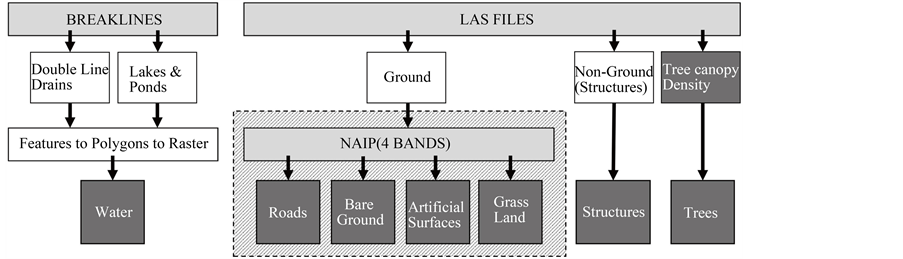
Figure 2. General procedure for land cover extraction from the different available datasets.
than 80%. In an attempt to improve the classification results, a supervised classification method was adopted. Therefore, the classification of the NAIP multispectral aerial photos using the ground only mask was then carried out using a Maximum Likelihood Classification (MLC) method. Training areas (77) were selected for a total of 15 different classes according to Table 1. The spectral signatures of those 15 classes were reviewed and, according to their separations, they were aggregated to 4 main classes, namely: artificial surfaces, bare ground, grassland, and roads and pavement. Shadow-covered areas were problematic since they were spectrally identified as a separate class. They represented all of the 4 main classes, but since Clarion County is mostly rural, it was assumed that the shadows represented mostly open Grassland.
The final signature file for all class aggregation was graphed, it showed a good separation in the multi-spec- tral aerial photo bands (1-4). Figure 3 depicts the spectral signatures of the aggregated classes. The signature

Table 1. General and specific classes of the training polygons for the supervised classification.

Figure 3. Line plot of the signature file of the aggregated classes.
file was saved and used in the general model as a reference to the supervised classification. This ensured the integrity of the classification and its uniformity when applied to any area of interest similar to Clarion County.
4.2. Assembly of Land Cover Classes
The last step for the land cover classification was to assemble all individually produced classes from LiDAR point cloud data, breaklines water polygons, and the NAIP MLC results into one final raster file. The Structures, Trees, Artificial Surfaces, Bare Ground, Grassland, Roads, and Water were all combined in one raster output (Table 2). Furthermore, the text description for each of the classes, the area in square feet, and the percent from total were calculated for each of the classes and added to the attribute table.
The tree cover was produced by aggregating all tree returns from the LiDAR point cloud data. Figure 4
Table 2. Final land cover classes and their corresponding symbol and description.
 (a1)
(a1) (a2)
(a2) (b1)
(b1) (b2)
(b2) (c1)
(c1)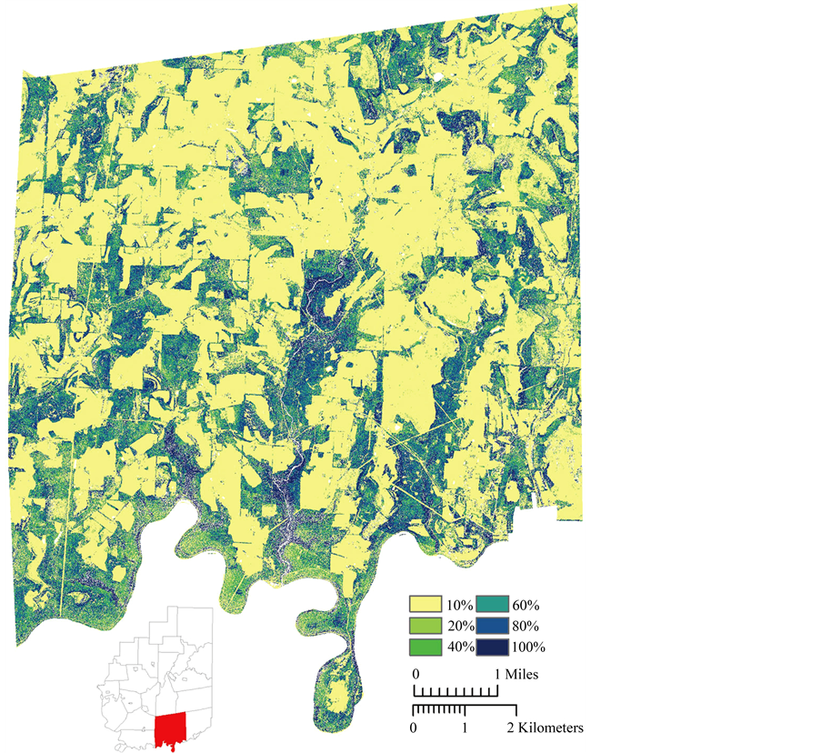 (c2)
(c2)
Figure 4. Land cover (1) and tree canopy density (2) results for the three selected pilot municipalities: Clarion Borough (a), Sligo Borough (b), and Porter Township (c).
shows the resulting land cover and tree canopy density maps for Clarion Borough (a1 and a2), Sligo Borough (b1 and b2), and Porter Township (c1 and c2) respectively.
4.3. Process Automation
A geoprocessing model was created during this process in order to automate the tasks that will be applied to different pilot study areas as well as for the whole county (Figure 5). The model was built using model tools (sub-models) that each would accomplish a certain task. Figure 4 shows the main model. It displays model tools for Study Area Definition, which identifies a specific municipality polygon that will be used in the process, Tree Density Extractor, which runs through the process of extracting and calculating tree percent coverage in relation to all LiDAR point cloud returns for a 10 ft × 10 ft cell size area, Tree Density Calculator, which calculates summary statistics for tree canopy coverage and percent densities, Trees and Structures Extractor, which collects information from the previous model tool and extracts tree only as well as ground only-covered areas, Ground Classifier, which runs through the MLC to extract the ground only land covers, and Land Cover Assembler, which combines all 7 extracted land covers from the previous model tools into one land cover map. The Random Points Generator model tool, on the other hand, was added in order to facilitate the generation of control points for accuracy assessment purposes, it is also used to extract the associated land cover class for each point.
Simple inputs and outputs were then defined and a user dialogue was created in order to simplify the process or running the model using other generic data from different municipalities throughout the state, given the availability of the base data needed to run the model (Figure 6). The geoprocessing model was then run on the three selected municipalities (Clarion and Sligo Boroughs, and Porter Township). Three land cover maps were produces along with their proper base information for the accuracy assessment.
4.4. Accuracy Assessment
An overall accuracy assessment was carried out for each of the three municipalities (Figure 1). Not all of the identified classes were present in all selected study areas. For example, Clarion Borough had some artificial surfaces that were located at the stadium as well as some of the outdoors tennis courts while they were absent in both Sligo Borough and Porter Township.
The geoprocessing model generated 300 random points within each of the selected municipalities and intersected them with the classification result to produce the reference data to ground truth checks. All ground truth

Figure 5. Main model: classifier and tree canopy extractor.
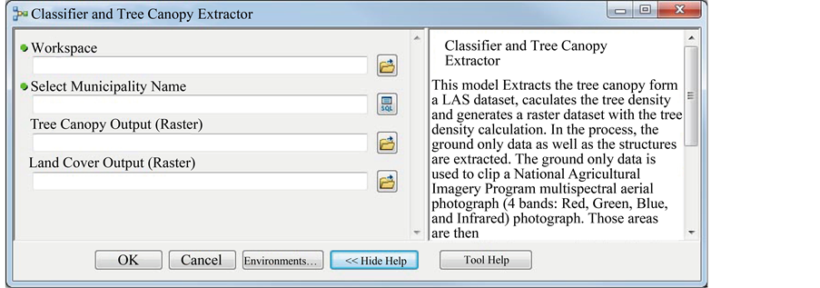
Figure 6. The main classifier and tree canopy extractor tool dialogue box.
data checks were carried out from the aerial photographs. Each point’s ground truth information was recorded and cross tabulated against the classified data for this specific point. The resulting accuracy assessment revealed an overall producer accuracy of 94.33% for the Clarion Borough, 94.67% for Sligo Borough, and 95.67% for Porter Township.
4.5. Land Cover and Tree Canopy Extractor Web Application
The aforementioned geoprocessing model was applied to all municipalities of Clarion County they were then mosaicked in order to produce one seamless datasets for land cover and tree canopy density. A web application was designed in a simple format in order to enable easy data access and extraction from both datasets. Map services were created using ArcGIS for Server and the application was built using ArcGIS Web AppBuilder Developer Edition.
Three geoprocessing tools were created: Land Cover Extractor and Tree Canopy Extractor, both of which clip the corresponding dataset according to a user-defined area of interest, and Download Land Cover and Tree Canopy, which mainly is designed to clip a user-defined area and to create a compressed geodatabase that include both datasets for later user exploration. Those models were created on the on the assumption that they will be shared through a geoprocessing service and that will be consumed in the web application.
4.6. The Web Application Interface
The published web interface (http://maps.clarion.edu/LandCoverExtractor) has widgets for all three geoprocessing tools. Additionally, two widgets were added to help printing the extracted area of interest using a custom page layout and to report information about the creation and the delivery of those datasets.
5. Conclusions
Land cover production is crucial to many applications. The methods used to produce those maps heavily rely on remotely sensed data and different classification algorithms. This study was an effort to produce a flexible and mostly automated method using hybrid techniques to handle high resolution multispectral aerial photographs combined with filtering LiDAR point cloud data. Although similar hybrid data were previously used to analyze wetland landscapes [33] with successful improvement of classification accuracies, but the techniques relied on object-based and decision tree modeling. Sinagra O. and Samsung L. (2014) also proved that using traditional classification methods of a variety of high resolution multispectral data combined with LiDAR helped in significantly improving the overall classification results of an urban environment in France [34] . At 1 m resolution, which is similar to the currently used datasets in the current project, Luo S. et al. (2016) argued that using supervised classification method on high resolution aerial photos combined with LiDAR derived images resulted in a significantly improved accuracy compared to coarser resolution datasets [37] . In the current study, using MLC on high resolution multispectral NAIP aerial photos and LiDAR point return filtering achieved satisfactory average accuracy of about 95% when applied on three relatively different landscapes that included forested areas, agricultural fields (including tilled fields), built up environment and open land.
On the other hand, the time difference between the NAIP (2010) and the LiDAR (2006) datasets has introduced some discrepancy in identifying some above-ground features especially with structures. The changes that happened during the 4-year difference were obvious in certain parts in the studied pilot municipalities. But overall it did not have any significant effects on the other classes nor on the overall classification. Additionally, the leaf-off LiDAR data used in this study have affected, in some extents, the results of classifying forested areas. The heterogeneity of the forests during leaf-off season introduced mixed results of detecting deciduous-covered areas. Those points were occasionally misidentified as structures. And although this misclassification was not generally detected by the adopted accuracy assessment method, they can be sporadically identified visually.
Furthermore, the automation of those methods helped in easily applying the land cover extraction to other municipalities in Clarion County. It is anticipated that the same geoprocessing models could be easily applied to future datasets when they become available. This study also opened the possibilities for sharing complex models with others through a local systems or a web application. And, although this study was designed using Clarion County municipalities, similar datasets are available for all Pennsylvania and, therefore, the generated geoprocessing model that produces the land cover as well as the tree canopy maps could be easily modified to accommodate any other county or region in the state. Also, this study could be certainly applied to any other state with similar datasets, especially the LiDAR LAS point cloud files and Breaklines, since the NAIP multispectral aerial photos are abundant throughout the United States.
Prospective Enhancements
Many enhancements could be accomplished in order to provide better data and improved processes to produce more accurate land cover and tree density maps. An updated set of data for input to the model might reveal more ways to enhance the classification process. For example, a 2013 multispectral NAIP aerial photographs is currently available, those can be used to either update the land cover map or to improve on the classification process by removing some of the uncertainty of the shadows between the two dates (2010 and 2013). It was not used in the current study due to the increased time difference it has compared to the statewide LiDAR data (2006). Also, this study could be extended and enriched if multiple classification methods (other than the MLC) are tested.
The developed web application was created using the Web AppBuilder for ArcGIS. The geoprocessing widgets used in this application could be enhanced in order to provide the following:
・ Automatic clearing of the display and the layer list from any previous process once a new one is started;
・ Provide feedback at the output level for each of the geoprocessing tasks (Land Cover Extractor (LC) and Tree Canopy Extractor (tC)) when the process is completed, as well as provide an option of printing the results without the use of the Print geoprocessing widget;
・ Enrich the application by adding functions that would graph the output results and summarize its tables in a printable format;
・ Unify the selection of the area of interest between all geoprocessing tasks instead of having to redraw the area of interest every time a process is run;
・ Provide extended help and assistance at multiple levels at each geoprocessing task;
・ Provide a user input form in order to collect suggestions on recommended enhancements of the application as well as the classification process.
In conclusion, this project demonstrated the possibilities of using process automation through the adoption of geoprocessing modeling techniques in order to produce land cover and tree canopy density maps, as well as in the dissemination of the results through the deployment of a web-based application. The adopted techniques produced land cover and tree canopy density maps at 10 ft × 10 ft (≈3 × 3 meters) spatial resolution due to the use of LiDAR data and high resolution multispectral aerial photographs. Land cover maps at similar high resolution are rarely found in Pennsylvania especially in rural and suburban environments. Using the web application, any interested user or agency can download the available data, the data can then be used and manipulated accordingly. The flexibility of the adopted methods would allow others to produce high resolution land cover and tree canopy density maps easily and in a timely manner.
Acknowledgements
Special thanks for Pennsylvania View (PAView), member of the America View program for funding this project. Also, the author would like to thank Devin Mendez, James McCall, and Glenn Wallace, all students at Clarion University of PA. Mr. Mendez helped in manipulating the land cover and tree canopy extractor model, testing it and ensuring its integrity at multiple stages of the project. Once the land cover raster images were extracted, Mr. McCall helped in conducting its accuracy assessment for Clarion Borough, Sligo Borough and for Porter Township. While Mr. Wallace worked on cleaning the LiDAR generated breaklines, ensuring their closure and converting them into polygons. Their efforts are greatly appreciated.
Cite this paper
Yasser M. Ayad, (2016) Developing an Automated Land Cover Classifier Using LiDAR and High Resolution Aerial Imagery. Journal of Geoscience and Environment Protection,04,97-110. doi: 10.4236/gep.2016.47011
References
- 1. Chrysoulakis, N., Feigenwinter, C., Triantakonstantis, D., Penyevskiy, I., Tal, A., Parlow, E., Fleishman, G., Düzgün, S., Esch, T. and Marconcini, M. (2014) A Conceptual List of Indicators for Urban Planning and Management Based on Earth Observation. ISPRS International Journal of Geo-Information, 3, 980-1002.
http://dx.doi.org/10.3390/ijgi3030980 - 2. Li, E., Du, P., Samat, A., Xia, J. and Che, M. (2015) An Automatic Approach for Urban Land-Cover Classification from Landsat-8 OLI Data. International Journal of Remote Sensing, 36, 5983-6007.
http://dx.doi.org/10.1080/01431161.2015.1109726 - 3. Haberman, D., Gillies, L., Canter, A., Rinner, V., Pancrazi, L. and Martellozzo, F. (2014) The Potential of Urban Agriculture in Montréal: A Quantitative Assessment. ISPRS International Journal of Geo-Information, 3, 1101-1117.
http://dx.doi.org/10.3390/ijgi3031101 - 4. Reimer, M. (2013) Planning Cultures in Transition: Sustainability Management and Institutional Change in Spatial Planning. Sustainability, 5, 4653-4673.
http://dx.doi.org/10.3390/su5114653 - 5. Wächter, P. (2013) The Impacts of Spatial Planning on Degrowth. Sustainability, 5, 1067-1079.
http://dx.doi.org/10.3390/su5031067 - 6. Ding, C., Wang, Y., Xie, B. and Liu, C. (2014) Understanding the Role of Built Environment in Reducing Vehicle Miles Traveled Accounting for Spatial Heterogeneity. Sustainability, 6, 589-601.
http://dx.doi.org/10.3390/su6020589 - 7. Piragnolo, M., Pirotti, F., Guarnieri, A., Vettore, A. and Salogni, G. (2014) Geo-Spatial Support for Assessment of Anthropic Impact on Biodiversity. ISPRS International Journal of Geo-Information, 3, 599-618.
http://dx.doi.org/10.3390/ijgi3020599 - 8. Florin, M., Murariu, G., Ionut, M. and Georgescu, L.P. (2011) Environment Monitoring through UAV Technologies. Analele Universitatii “Dunarea de Jos” Galati. Fascicle II: Mathematics, Physics, Theoretical Mechanics, 34, 300-308.
- 9. Lederwasch, A. and Mukheibir, P. (2013) The Triple Bottom Line and Progress toward Ecological Sustainable Development: Australia’s Coal Mining Industry as a Case Study. Resources, 2, 26-38.
http://dx.doi.org/10.3390/resources2010026 - 10. Lei, L. and Hilton, B. (2013) A Spatially Intelligent Public Participation System for the Environmental Impact Assessment Process. ISPRS International Journal of Geo-Information, 2, 480-506.
http://dx.doi.org/10.3390/ijgi2020480 - 11. Liang, X., Hyyppä, J., Kaartinen, H., Holopainen, M. and Melkas, T. (2012) Detecting Changes in Forest Structure over Time with Bi-Temporal Terrestrial Laser Scanning Data. ISPRS International Journal of Geo-Information, 1, 242-255.
http://dx.doi.org/10.3390/ijgi1030242 - 12. Ahmed, B. and Ahmed, R. (2012) Modeling Urban Land Cover Growth Dynamics Using Multi-Temporal Satellite Images: A Case Study of Dhaka, Bangladesh. ISPRS International Journal of Geo-Information, 1, 3-31.
http://dx.doi.org/10.3390/ijgi1010003 - 13. Yeshaneh, E., Wagner, W., Exner-Kittridge, M., Legesse, D. and Blöschl, G. (2013) Identifying Land Use/Cover Dynamics in the Koga Catchment, Ethiopia, from Multi-Scale Data, and Implications for Environmental Change. ISPRS International Journal of Geo-Information, 2, 302-323.
http://dx.doi.org/10.3390/ijgi2020302 - 14. Forsythe, K.W. and McCartney, G. (2014) Investigating Forest Disturbance Using Landsat Data in the Nagagamisis Central Plateau, Ontario, Canada. ISPRS International Journal of Geo-Information, 3, 254-273.
http://dx.doi.org/10.3390/ijgi3010254 - 15. Forsythe, K.W., Schatz, B., Swales, S.J., Ferrato, L.-J. and Atkinson, D.M. (2012) Visualization of Lake Mead Surface Area Changes from 1972 to 2009. ISPRS International Journal of Geo-Information, 1, 108-119.
http://dx.doi.org/10.3390/ijgi1020108 - 16. Tran, H., Tran, T. and Kervyn, M. (2015) Dynamics of Land Cover/Land Use Changes in the Mekong Delta, 1973-2011: A Remote Sensing Analysis of the Tran Van Thoi District, Ca Mau Province, Vietnam. Remote Sensing, 7, 2899-2925.
http://dx.doi.org/10.3390/rs70302899 - 17. Setiawan, Y., Rustiadi, E., Yoshino, K., Liyantono and Effendi, H. (2014) Assessing the Seasonal Dynamics of the Java’s Paddy Field Using MODIS Satellite Images. ISPRS International Journal of Geo-Information, 3, 110-129.
http://dx.doi.org/10.3390/ijgi3010110 - 18. Prilepova, O., Hart, Q., Merz, J., Parker, N., Bandaru, V. and Jenkins, B. (2014) Design of a GIS-Based Web Application for Simulating Biofuel Feedstock Yields. ISPRS International Journal of Geo-Information, 3, 929-941.
http://dx.doi.org/10.3390/ijgi3030929 - 19. Yen, H., Sharifi, A., Kalin, L., Mirhosseini, G. and Arnold, J.G. (2015) Assessment of Model Predictions and Parameter Transferability by Alternative Land Use Data on Watershed Modeling. Journal of Hydrology, 527, 458-470.
http://dx.doi.org/10.1016/j.jhydrol.2015.04.076 - 20. Ongsomwang, S. and Pimjai, M. (2015) Land Use and Land Cover Prediction and Its Impact on Surface Runoff. Suranaree Journal of Science and Technology, 22, 205-223.
- 21. Halmy, M.W.A., Gessler, P.E., Hicke, J.A. and Salem, B.B. (2015) Land Use/Land Cover Change Detection and Prediction in the North-Western Coastal Desert of Egypt Using Markov-CA. Applied Geography, 63, 101-112.
http://dx.doi.org/10.1016/j.apgeog.2015.06.015 - 22. Machala, M., Honzová, M. and Klimánek, M. (2015) Generating Land-Cover Maps from Remotely Sensed Data: Manual Vectorization versus Object-Oriented Automation.
- 23. Sun, L. and Schulz, K. (2015) The Improvement of Land Cover Classification by Thermal Remote Sensing. Remote Sensing, 7, 8368-8390.
http://dx.doi.org/10.3390/rs70708368 - 24. Babamaaji, R. and Lee, J. (2014) Land Use/Land Cover Classification of the Vicinity of Lake Chad Using NigeriaSat-1 and Landsat Data. Environmental Earth Sciences, 71, 4309-4317.
http://dx.doi.org/10.1007/s12665-013-2825-x - 25. Jing, L. and Yi, L. (2015) Hyperspectral Remote Sensing Images Terrain Classification in DCT SRDA Subspace. The Journal of China Universities of Posts and Telecommunications, 22, 65-71.
http://dx.doi.org/10.1016/S1005-8885(15)60626-4 - 26. Salah, M., Trinder, J.C. and Shaker, A. (2011) Performance Evaluation of Classification Trees for Building Detection from Aerial Images and LiDAR Data: A Comparison of Classification Trees Models. International Journal of Remote Sensing, 32, 5757-5783.
http://dx.doi.org/10.1080/01431161.2010.507678 - 27. Panda, S.S., Hoogenboom, G. and Paz, J.O. (2010) Remote Sensing and Geospatial Technological Applications for Site-Specific Management of Fruit and Nut Crops: A Review. Remote Sensing, 2, 1973-1997.
http://dx.doi.org/10.3390/rs2081973 - 28. Gu, Y., Wang, Q., Jia, X. and Benediktsson, J.A. (2015) A Novel MKL Model of Integrating LiDAR Data and MSI for Urban Area Classification. IEEE Transactions on Geoscience and Remote Sensing, 53, 5312-5326.
http://dx.doi.org/10.1109/TGRS.2015.2421051 - 29. Díaz-Vilariño, L., González-Jorge, H., Bueno, M., Arias, P. and Puente, I. (2016) Automatic Classification of Urban Pavements Using Mobile LiDAR Data and Roughness Descriptors. Construction and Building Materials, 102, 208-215.
- 30. Arroyo, L.A., Phinn, S., Armston, J. and Johansen, K. (2010) Integration of LiDAR and QuickBird Imagery for Mapping Riparian Biophysical Parameters and Land Cover Types in Australian Tropical Savannas [Electronic Resource]. Forest Ecology and Management, 259, 598-606.
http://dx.doi.org/10.1016/j.foreco.2009.11.018 - 31. Lin, Y. and Hyyppä, J. (2016) A Comprehensive but Efficient Framework of Proposing and Validating Feature Parameters from Airborne LiDAR Data for Tree Species Classification. International Journal of Applied Earth Observation and Geoinformation, 46, 45-55.
http://dx.doi.org/10.1016/j.jag.2015.11.010 - 32. Schumacher, J. and Nord-Larsen, T. (2014) Wall-to-Wall Tree Type Classification Using Airborne Lidar Data and CIR Images. International Journal of Remote Sensing, 35, 3057-3073.
http://dx.doi.org/10.1080/01431161.2014.894670 - 33. Rapinel, S., Hubert-Moy, L. and Clément, B. (2015) Combined Use of LiDAR Data and Multispectral Earth Observation Imagery for Wetland Habitat Mapping. International Journal of Applied Earth Observation and Geoinformation, 37, 56-64.
http://dx.doi.org/10.1016/j.jag.2014.09.002 - 34. Sinagra, O. and Lim, S. (2014) Data Fusion and Supervised Classifications with Lidar Data and Multispectral Imagery. Proceedings of the 14th International Multidisciplinary Scientific GeoConference SGEM, 3, 129-136.
- 35. NAIP Imagery. [Online].
http://www.fsa.usda.gov/programs-and-services/aerial-photography/imagery-programs/naip-imagery/ - 36. PASDA—The Pennsylvania Spatial Data Clearinghouse. [Online].
http://www.pasda.psu.edu/ - 37. Luo, S.Z., Wang, C., Xi, X.H., Zeng, H.C., Li, D., Xia, S.B. and Wang, P.H. (2016) Fusion of Airborne Discrete-Return LiDAR and Hyperspectral Data for Land Cover Classification. Remote Sensing, 8, 1-19.