ABSTRACT

Nowadays, more and more electrical power is being distributed to customers by underground cables rather than overhead transmission lines due to their advantage of providing better protection in inclement weather. They also have significantly reduced electromagnetic field emission because of their copper shielding. But underground cables have larger capacitance than transmission lines per unit. Thus, ferroresonance is more likely to occur in distribution systems using underground cables. Moreover, soil humidity at a depth of one meter remains 100 percent for most of the year, a factor that risks the occurrence of water tree (WT) in cables. Consequently, both ferroresonance and WT are prone to occur in underground cable systems. The objective of this paper is to determine the relationship between ferroresonance and water tree. A test system was designed to simulate and analyze ferroresonance in a cable system caused by single-phase switch and water tree. Eight scenarios of water tree were compared in the simulation. There sponses of ferroresonance are presented in this paper and two common patterns are observed from the simulation results.

Keywords:

Ferroresonance, Water Tree, PSCAD, COMSOL, Overvoltage

1. Introduction

In recent decades, technology has been more and more focused on decreasing power losses in the power-delivery process, taking into account both economic and ecological conditions. However, we have to realize the fact that the lower the losses, the smaller the damping resistive load. So the delivery process will become more sensitive to different types of transient behaviors, and more susceptible to failure. Ferroresonance is one of these failures and it is occurring in more and more situations [1] [2] .

Ferroresonance is a nonlinear phenomenon that can generate overvoltage, over current, and harmonic distortion, which is normally caused by single-pole switch in light loaded system. The first paper to discuss ferroresonance was published in 1907 [3] , and the term was first used in 1920 [4] . The phenomenon received wide attention in 1937 [5] . The first analytical paper related to ferroresonance was presented in 1950 [6] . Other important papers were published later and mainly concentrated on two areas: increasing the accuracy level of transformer modeling, and studying the ferroresonance phenomenon at the whole system level [7] . From all above papers, we know that ferroresonance is caused by single pole switch and it highly depends on the magnitude of losses and transformer connection methods. Although these papers have addressed ferreresonance, none of them have focused on the influence of abnormal factors such as water tree and other types of faults. So the objective of this paper is to determine the relationship between ferroresonance and faults like WT.

In this paper, ferroresonance caused by single-phase switch and influenced by different water-tree conditions is simulated and analyzed in PSCAD simulation software. Eight different scenarios were compared and analyzed in detail.

2. Theoretical Principles

2.1. Ferroresonance

Ferroresonance is a highly nonlinear phenomenon in a distribution system. It takes place in all systems that include saturable ferromagnetic inductors, neutral or shunt capacitors and light load, which are shown in Figure 1. It can cause either a short transient or continuous overvoltage and over current that can reach up to 4 to 6 times the normal values. It also causes thermal problems in electrical equipment as well as loud noise [2] .

In power systems, the iron core of the power or voltage transformer is the saturable inductor. In addition, plenty of equipments are capacitive devices such as the neutral capacitance of underground cables, and shunt capacitors. Moreover,

ferroresonance has a greater chance of occurring in a light load or non-load system. If significant losses exist in the system, ferroresonance can be damped out by the resistive load. For example, in a one phase open condition, a resistive load of 4 percent of the transformer capacity can eliminate the overvoltage of ferroresonance [8] . Additionally, the type of winding configuration in a transformer can also influence ferroresonance [8] [9] . So changing transformer connection method can also eliminate ferroresonance.

Plenty of circuit structures can result in this nonlinear resonance phenomenon. Jacobson presented seven types of circuits in danger of ferroresonance [10] . One of them is selected in this paper to simulate the ferroresonance process, as its circuit structure shown in Figure 2. In this system, a voltage source is connected to a non-loaded transformer through long distance underground three- phase cables or overhead transmission lines. After an instant of switching occurred on phase A, phase B and phase C’s core inductors are charged through their cables. At that moment, these neutral capacitors become a short circuit, and the current goes through the transformer’s winding between phase A-B and phase A-C. Because the transformer has a saturable iron core, the nonlinear inductor could become saturated when voltage increases. The saturation can cause considerable current propagation through the transformer and the series resonance circuit forms. Then the voltage decreases, and the inductors become unsaturated. During the periods that follow, the transformer windings become saturated and unsaturated again [11] [12] .

This process can be understood easily by assuming the transformer is a flux-controlled switch [13] . When the flux is below the saturation point, the switch is open. So the AC source and capacitance are connected by a high loss resistance. Then the flux increases linearly before the core is saturated. At that instant, the flux-controlled switch will be closed, the capacitance discharges to the AC source via the core inductor, and the L-C resonance circuit structure is formed, which will cause overvoltage and over current. Repetition of this process will finally cause the failure of transformer.

2.2. Water Tree

Underground cables have the advantage of better protection in inclement weather and a significantly reduced electromagnetic field emission due to their copper shielding. However, cables are normally deeply buried in the soil and are therefore difficult to monitor and repair. It is necessary to monitor cables for all potential problems that might happen during their lifetime.

WT, a failure that occurs in the insulation layer of underground cables [14] , is one of the severest and most common faults. There are two kinds of WT: bowtie and vented WT. In this paper, the focus is only on the first type since it is the most dangerous one [15] . WT forms in solid dielectric materials such as cross- link polyethylene (XLPE) [16] . It occurs when the surrounding humidity is higher than 65 percent [17] . Starting from small voids, it grows slowly by increasing the surrounding electrical field and producing voltage stress at this point. Then some microfractures occur and are filled with water. The WT keeps growing in a tree shape until it reaches the conductor. Then high impedance fault happens and eventually causes the failure of cables.

To simulate water-tree fault in PSCAD software, a lumped parameter method was employed. A widely used water-tree model involves a parallel resistor and capacitor [15] [18] [19] [20] . The values of equivalent resistance and capacitance are calculated by simulating the water-tree cable in COMSOL software, which is a powerful multi-physics fields modeling software.

In this paper, shield cables with parameters of 37 strands, 750 kcmil were selected for the simulation. They were assumed to be buried at a depth of 36 inches and the distance between each was set at 7.5 inches. This type of cable includes an aluminum conductor, XLPE insulation and a copper-shield layer. The parameters of such cables are referenced on the website of the Okonite company [21] .

In order to model the WT cables in PSCAD, the equivalent resistance and capacitance should be determined. They are decided by the relative permittivity and electrical conductivity of WT. Based on [14] [20] [22] we know that the maximum electrical conductivity of WT is 10¹⁰ times the conductivity of XLPE and the largest relative permittivity of WT is 3 times the permittivity of XLPE. The peak value occurs at the beginning point and decreases linearly to the edge of water-tree area. These features can be simulated in COMSOL as shown in Figure 3.

After building the physical model with its material characteristics, the equivalent capacitance and resistance of WT can be calculated in COMSOL. The cable conductor is connected to a 15 kV voltage source, and the shield layer is grounded. The water-tree region is assumed to be 1mm. It is noted that the capacitance of WT increases and the resistance of WT decreases linearly when the region is increased. The capacitance of the WT can be calculated by the relative permittivity, and the resistance can be determined from conductivity.

The capacitance and conductance are solved by these equations [14] :

$C=\frac{2\text{π}{\epsilon }_r{\epsilon }_{0}L}{\ln \left(r_2/r_1\right)}$ (1)

$G=\sigma A/L$ (2)

where $r_1$ is the radius of the cable conductor, $r_2$ is the radius of the insulation, A is the cross-section area of the cable conductor, $\sigma$ is the conductivity, ${\epsilon }_r$ is the relative permittivity, ${\epsilon }_0$ is the permittivity of vacuum, and $L$ is the length of the cable conductor.

Figure 4 demonstrates that the resistance decreases and the capacitance increases when the WT length is developing from 50 percent to 100 percent in the insulation layer. It shows that the resistance remains around $2.3{\text{e}}^7\Omega$ and decreases significantly when it touches the conductor. Moreover, the capacitance hardly changes. It increases from $3.504{\text{e}}^{-13}\text{F}$ to $3.517{\text{e}}^{-13}\text{F}$ . During the simulation of WT in PSCAD, $7.9{\text{e}}^6\Omega$ and $3.517{\text{e}}^{-13}\text{F}$ are used as the equivalent resistance and capacitance.

3. Simulation of Ferroresonance Using PSCAD

Ferroresonance is a highly nonlinear process because of the nonlinear characteristics of the saturable iron core. It includes a large number of nonlinear features, such as steady state responses existing for the same given parameters; different frequency of voltage and current wave-forms; and jump resonance [23] .

Thus, linear analytical methods are not suitable to analyze ferroresonance for its abnormal responses. A more fitting method for analyzing this process is the use of simulation software. Fortunately, a simulation tool can provide accurate response and the capability of studying ferroresonace behavior.

PSCAD software is used to simulate ferroresonance influenced by water tree in this paper. This paper employed a similar circuit, which is introduced above in Part 2.1. But in order to investigate the influence on the process of other factors, like faults, a water-tree cable is built in this system. It is known that low impedance faults can cause blown fuses, which are easy to detect and repair. A more dangerous and unpredictable type of fault is a high impedance fault like

WT. It can be present in power systems for a long time without causing failure [24] . However, the existence of water tree can have a significant influence on the ferroresonance response, because WT is composed of a parallel capacitance and resistance and thus it can influence the value of resonance circuit and then influence the ferroresonance response. Moreover, different WT conditions will form different resonance situations and cause different results.

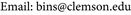
This situation is simulated in PSCAD platform. The equivalent source system is connected with a light load saturable transformer by a 5 km distance underground three-phase cables. The configuration of the ferroresonance circuit is shown in Figure 5.

4. Results

The response of ferroresonance depends on many factors and conditions, which are fully discussed in previous papers, such as voltage magnitude, voltage frequency and capacitance of the system. However, different conditions of water tree will also influence the response. For example:

1) Water tree position. The water tree can take shape anywhere from the beginning to the end of a cable. Different positions will cause different ferroresonance wave-forms.

2) Water tree phase. The single-pole switch happens on one phase, but the water tree can generate on all three phases. The water tree and single-pole switch occur on the same phase or different phases will cause different results.

In this paper, a ferroresonance circuit, including an equivalent source system, 5 km length three-phase cables, 1 mm water tree, a saturable nonlinear transformer and a light load is simulated in PSCAD, which is shown in Figure 5. The single-pole switch happens at 0.3 second on phase B, and the water tree can take place at any position of the cables and any phase.

Figure 6 shows the ferroresonance results of this cable distribution system when WT is located at different positions of phase A cable, from the beginning point of the cable to the ending point. The cable is divided into seven same length parts and each time the WT locates at different points and all other conditions remain unchanged. It is noticed each time the same length is moved (about 0.7 km). When the water tree is located at either end of a cable, as long as the WT location is different, the ferroresonance over voltage profile will change

markedly. The overvoltage happens at 1.3 second, when WT is located at 0.7 km from the starting end in Figure 6(a). But the overvoltage occurs at 0.55 seconds if the WT is 1.4 km from the beginning point as shown in Figure 6(b). Similar results are found in Figure 6(e) and Figure 6(f). When the WT is located 1.4 km from the ending point, the ferroresonance takes place at 0.8 seconds; but it occurs at 1.05 seconds if WT is located at 0.7 km from the end of the cable. When the WT lies in the middle of a cable and moves the same length, the ferroresonance response is almost the same. From Figure 6(c) and Figure 6(d), it is noticed that even when the WT is located at different positions, the voltage profiles are almost exactly the same. Similar results have been proved in other lengths of cables (from 1 km to 8 km).

Figure 7 indicates the different outcomes when WT and ferroresonance occur on the same cable or different cables. All other conditions are the same. These figures demonstrate that if these two phenomena occur in the same cable, more overvoltage will be generated compared with on different cables. From Figure 6(f) and Figure 7(b) we can see that if these two phenomena occur on different cables, the overvoltage takes place around 1 second. But if they happen on the same cable, the overvoltage occurs at 0.5 second and more overvoltage is included, as shown in Figure 7(a). Similar results are observed in other lengths of cables.

5. Conclusions

Ferroresonance occurs more and more frequently nowadays because technical development tends toward decreasing losses during power transmission. Water tree has a significant influence on the ferroresonance phenomenon. This paper presents detailed simulation of ferroresonance and water tree. Impacts of various water tree conditions on ferroresonance have been analyzed as well. Two common patterns are observed from the results. Firstly, the location of water tree has a significant influence on the ferroresonance response. If WT occurs at each end

of a cable, ferroresonance response changes a lot as long as the WT happens at different positions. But if the WT happens in the middle of a cable, even at different locations, the ferroresonance response is similar. Secondly, these two phenomena, occurring on the same cable or different cables, also have an effect on the results. If they take place in the same cable, more overvoltage occurs compared with that in different cables.

In the future, additional different lengths of cables will be studied, and the influence of nonlinear load and transformer connection methods will be analyzed.

Acknowledgements

The authors would like to thank all the members of the Clemson University Power Research Association (CUEPRA) for their guidance, data and financial support for this research.

Cite this paper

Sun, B., Makram, E. and Xu, X.F. (2017) Impacts of Water-Tree Fault on Ferroresonance in Underground Cables. Journal of Power and Energy Engineering, 5, 75-86. https://doi.org/10.4236/jpee.2017.512010

References

- 1. Bertini, G.J. (2006) Molecular Thermodynamics of Water in Direct-Buried Power Cables. IEEE Electrical Insulation Magazine, 22, 17-23. https://doi.org/10.1109/MEI.2006.253417
- 2. Dugan, R.C. (2003) Examples of Ferroresonance in Distribution Systems. 2003 IEEE Power Engineering Society General Meeting (IEEE Cat. No. 03CH37491), 2, 1-3.
- 3. Bethenod, J. (1907) Sur le transformateur et resonance. L’Eclairae Electr., 289-296.
- 4. Boucherot, P. (1920) Existence de deux régimes enferro-résonance. R.G.E., 827-828.
- 5. Butler, J.W. and Concordia, C. (1937) Analysis of Series Capacitor Application Problems. Transactions of the American Institute of Electrical Engineers, 56, 975-988. https://doi.org/10.1109/T-AIEE.1937.5057677
- 6. Rudenberg, R. (1950) Transient Performance of Electric Power Systems. McGraw-Hill, New York.
- 7. Iravani, M.R., Chaudhary, A.K.S., Giesbrecht, W.J., Hassan, I.E., Keri, A.J.F., Lee, K.C., Martinez, J.A., Morched, A.S., Mork, B.A., Parniani, M., Sharshar, A., Shirmohammadi, D., Walling, R.A. and Woodford, D.A. (2000) Modeling and Analysis Guidelines for Slow Transients—Part III: The Study of Ferroresonance. IEEE Transactions on Power Delivery, 15, 255-265. https://doi.org/10.1109/61.847260
- 8. Dugan, R.C., McGranaghan, M.F., Santoso, S. and Beaty, H.W. (2003) Electrical Power Systems Quality. 2nd Edition, McGraw-Hill.
- 9. Smith, D.R., Swanson, S.R. and Borst, J.D. (1975) Overvoltages with Remotely- Switched Cable-Fed Grounded Wye-Wye Transformers. IEEE Transactions on Power Apparatus and Systems, 94, 1843-1853. https://doi.org/10.1109/T-PAS.1975.32030
- 10. Jacobson, D.A.N. (2003) Examples of Ferroresonance in a High Voltage Power System. 2003 IEEE Power Engineering Society General Meeting (IEEE Cat. No. 03CH37491), 2, 1-7.
- 11. Bátora, B. and Toman, P. (2013) Using of PSCAD Software for Simulation Ferroresonance Phenomenon in the Power System with the Three-Phase Power Transformer. Transactions on Electrical and Electronic Engineering, 2, 102-105.
- 12. Thanomsat, N. and Plangklang, B. (2016) Ferroresonance Phenomenon in PV System at LV Side of Three Phase Power Transformer using of PSCAD Simulation. Electrical Engineering/Electronics, Computer, Telecommunications and Information Technology, 28 June-1 July 2016. https://doi.org/10.1109/ECTICon.2016.7561384
- 13. Walling, R.A. (2003) Ferroresonance in Low-Loss Distribution Transformers. IEEE General Meeting on Power Engineering Society, Vol. 2, 1220-1222. https://doi.org/10.1109/PES.2003.1270502
- 14. Burkes, K.W. (2014) Water Tree Analysis and On-Line Detection Algorithm Using Time Domain Reflectometry. M.S. Thesis, Clemson University.
- 15. Mejía, J.C.H. (2008) Characterization of Real Power Cable Defects by Diagnostic Measurements. Ph.D. Diss., Georg. Inst. Technol.
- 16. Burkes, K.W., Makram, E.B. and Hadidi, R. (2015) Water Tree Detection in Underground Cables Using Time Domain Reflectometry. IEEE Power and Energy Technology Systems Journal, 2, 53-62. https://doi.org/10.1109/JPETS.2015.2420791
- 17. Steennis, E.F. and Kreuger, F.H. (1990) Water Treeing in Polyethylene Cables. IEEE Transactions on Electrical Insulation, 25, 989-1028. https://doi.org/10.1109/14.59869
- 18. Kawai, J. and Wire, S.E. (2001) Relative Permittivity and Conductivity of Water-Treed Region in Cross-Linked Polyethylene. Proceedings of the IEEE 7th International Conference on Solid Dielectrics, 25-29 June 2001, 163-166.
- 19. Arief, Y.Z., Shafanizam, M., Adzis, Z. and Makmud, M.Z.H. (2012) Degradation of Polymeric Power Cable Due to Water Treeing under AC and DC Stress. IEEE International Conference on Power and Energy, 2-5 December 2012, 950-955.
- 20. Ozaki, S.N.T., Ito, N., Sengoku, I. and Kawai, J. (2001) Changes of Capacitance and Dielectric Dissipation Factor of Water-Treed XLPE with Voltage. International Symposium on Electrical Insulating Materials, 22 November 2001, 459-462. https://doi.org/10.1109/ISEIM.2001.973702
- 21. The Okonite Company. http://okonite.com/Product_Catalog/section2/section2-pdfs/2-10.pdf
- 22. Toyoda, T., Mukai, S., Ohki, Y., Li, Y. and Maeno, T. (2001) Estimation of Conductivity and Permittivity of Water Trees in PE from Space Charge Distribution Measurements. IEEE Transactions on Dielectrics and Electrical Insulation, 8, 111-116. https://doi.org/10.1109/94.910433
- 23. Sakarung, P. and Chatratana, S. (2005) Application of PSCAD/EMTDC and Chaos Theory to Power System Ferroresonance Analysis. International Conference on Power Systems Transients, June 2005, No. 227, 19-23.
- 24. Densley, J. (2001) Ageing Mechanisms and Diagnostics for Power Cables—An Overview. IEEE Electrical Insulation Magazine, 17, 14-22. https://doi.org/10.1109/57.901613