Journal of Applied Mathematics and Physics
Vol.07 No.03(2019), Article ID:91068,14 pages
10.4236/jamp.2019.73037
Simplified Integral Calculations for Radial Fin with Temperature-Dependent Thermal Conductivity
Okey Oseloka Onyejekwe
Computational Science Program Addis Ababa University, Arat Kilo Campus, Addis Ababa, Ethiopia

Copyright © 2019 by author(s) and Scientific Research Publishing Inc.
This work is licensed under the Creative Commons Attribution International License (CC BY 4.0).
http://creativecommons.org/licenses/by/4.0/


Received: February 11, 2019; Accepted: March 9, 2019; Published: March 12, 2019
ABSTRACT
Numerical solution of a radiative radial fin with temperature-dependent thermal conductivity is presented. Calculations are implemented along the lines of a boundary integral technique coupled with domain discretization. Localized solutions of the nonlinear governing differential equation are sought on each element of the problem domain after enforcing inter-nodal connectivity as well as the boundary conditions for the dependent variables. A finite element-type assembly of the element equations and matrix solution yield the scalar profile. Comparison of the numerical results with those found in literature validates the formulation. The effects of such problem parameters as radiation-sink temperature, thermal conductivity, radiation-conduction fin parameter, volumetric heat generation, on the scalar profile were found to be in conformity with the physics of the problem. We also observed from this study that the volumetric heat generation plays a significant role in the overall heat transfer activity for a fin. For relatively high values of internal heat generation, a situation arises where a greater percentage of this energy can not escape to the environment and the fin ends up gaining energy instead of losing it. And the overall fin performance deteriorates. The same can also be said for the radiation-conduction parameter , whose increases can only give physically realistic results below a certain threshold value.
Keywords:
Radiative Radial Fin, Temperature-Dependent Thermal Conductivity, Discretized Problem Domain, Boundary Integral Technique, Generic Elements, Assembly of Element Equations

1. Introduction
Fins are vastly used in different heat transfer applications such as air-conditioning systems, heat exchangers, power plants, refrigeration, chemical processing equipment, computers, fluid-conveyance structures etc. Their chief purpose is the transfer of heat from a surface to the surrounding. This process is usually enhanced by attaching highly conductive materials to a surface in order to facilitate heat flow between a source and a sink. Though linear differential equations can be used to model rectangular fins, however thermal conductivity is known to depend on temperature because of the high temperature gradient that exists in fin operation. The heat transfer coefficient should therefore reflect the temperature variation along the fin or the local temperature difference between the fin and the surrounding fluid. Since this is a highly significant consideration, we should end up considering a nonlinear differential equation for modelling fin energy transfer performance and thermal optimization [1] [2] . Fin research has broadly developed into two major areas namely: optimal representation of fin profiles [3] [4] [5] [6] and consideration of thermal characteristics [7] [8] [9] [10] . In this regard, rectangular fins are the most studied, not only because of their relatively easier mathematical representation but also their uncomplicated manufacturing procedure. Other considerations which lead to the analysis of other shapes include efficiency and the possession of thermo-physical characteristics that enhance fin design. Treatment of trapezoidal profiles as triangular in order to render the governing equation solvable is worthy of mention (Kraus et al. [11] ). This approach led to a wrong treatment of the boundary condition and therefore wrong results (see comments in [12] ). Rusagara and Harley [13] got rid of this issue by providing a well balanced numerical scheme that dealt with a proper form of the triangular fin. The incorporation of zero flux condition into their so called well balanced numerical scheme and the validity of the solutions for a triangular fin confirmed the originality of their work. Khani and Aziz [10] developed a homotopy analysis method (HAM) for the thermal performance of a trapezoidal fin in which both the thermal conductivity and the heat transfer coefficient are temperature dependent. Their solution was found to be superior to an earlier attempt [14] . A comprehensive study of a radial fin with rectangular and hyperbolic profiles was carried out by Moitsheki [15] . Both the thermal conductivity and heat transfer coefficient were considered to be power laws and temperature dependent. The resulting nonlinear problems were analyzed by Lie symmetry technique. His work not only provided faithful benchmark solutions but significant addition to existing closed form solutions. Both the initial and boundary conditions considered in [15] did not remain invariant; as a result, a numerical approach was adopted to solve this problem. His results displayed some interesting observations including the inability of the scalar profile to display adiabatic conditions for long periods of time. His overall approach had earlier been inferred to by Arslanturk [16] in his optimum design of space radiators with temperature-dependent thermal conductivity. This is remarkable because the governing equations that usually describe energy transfer for fins were also found to be applicable in handling the immense heat generated during a space vehicle entry into the earth’s atmosphere.
The other broad area of fin literature focuses on the fin’s thermophysical properties for any chosen geometry. Some of the work treated in this area, involved the use of analytic and semi analytic techniques in predicting the fin’s scalar profiles especially for idealized cases. Atay and Coskun [17] carried out a comparative analysis of power-law fin-type problems using both the variational iteration method as well as the finite element technique. Their case studies showed that an increase in nonlinearity arising from and the increase of certain problem parameters resulted in an increase in error values for both methods. Having made this observation, their overall results showed a good agreement between the variational iteration technique and the finite element method. Aziz and Enamul-Huq [18] in an earlier study, adopted a perturbation techniques to solve a fin problem involving pure convection and temperature-dependent thermal conductivity. Aziz [19] later included a uniform heat generation term in the governing equation. Pozzesh et al. [20] used the differential transformation method (DTM) to study the efficiency of a convective-radiative fin with temperature dependent thermal conductivity and successfully carried out parametric studies for various problem parameters. The problem of heat enhancement in annular fins using functionally graded material was considered by Hassanzadeh and Pekel [21] . They considered the thermal conductivity of the annular fin to obey a power-law function; and replaced the variable coefficients related to the second and third terms of the governing differential equation by their mean-values. Their studies led them to the conclusion that the temperature gradient for the functionally graded annular fin is lower for the non-graded or homogeneous case. They also determined that an increase in the fin inhomogeneity parameter decreased the thermal resistance along the fin radius. Their study led them to conclude that for a functionally graded fin, the heat transfer between the annular fin and surrounding fluid was more efficient in comparison with the homogeneous annular fin.
Considerable work has also been devoted to the application of domain-based numerical techniques to fin study and analysis since most of the analytic and semi-analytic methods contain complex terms which may not be convenient for fin design. For example the finite difference technique presents an accurate and a straight forward way to resolve nonlinear fin equations (Jain et al. [22]). Sobamowo [23] adopted a MATLAB finite-difference solution of the fin equation. His results confirmed that the fin temperature distribution, total heat transfer and fin efficiency were all significantly affected by the thermo-geometric properties of the fin. And that for a thermally stable scalar profile, the fin thermo-geometric parameter must not exceed a specific value. In addition, he determined that from his results, that an increase in the fin internal heat generation values affected the stability range of the thermo-geometric parameter. In a later work, Oguntala and Sobamowo [24] used the Galerkin’s method of weighted residual to study the temperature distribution of a rectangular fin with temperature-dependent thermal properties and internal heat generation. Their results displayed a monotonic drop in scalar profiles for various thermo-geometric, thermal conductivity and convective heat transfer parameters. They further conducted various parametric studies related to the fin ability to conduct heat. These studies show that larger values of the fin thermo-geometric properties guarantee better heat convection along the fin length. And for cases where there is a negligible heat loss from the fin tip to the environment, the fin temperature decreases along the fin length.
It comes as no surprise that earlier work in fin calculations were phrased in terms of finite difference schemes. It was only after the numerical advantages of integral formulations became apparent that attempts to use boundary integral and finite element became widespread. This trend has caught up so fast in the field of solid mechanics to the extent that approximations based solely on finite-difference approximations are hardly ever used. This is however not the case in fluid dynamical computations where the oftentimes the nonlinear inertia terms renders the governing equations non-self adjoint and as a result differential approximations come as a natural choice.
In the work reported herein, we adopt a domain-decomposed singular integral formulation to solve the one-dimensional nonlinear fin equation whose complimentary equation comprises a one-dimensional Poisson equation with a dirac-delta forcing function. Its solution is known as the fundamental solution and together with the Green’s second identity yield the basis for the integral representation of the governing equation in a generic element of the discretized problem domain. The boundary integral representation of the governing equation on each element of the discretized domain is similar to a finite element system of equations and come with all the advantages and properties of the finite element method (FEM) ability of dealing with nonlinearity and non-homogeneity. The classic nonlinear fin equation with a temperature dependent thermal conductivity is solved and the results are validated through the use of benchmark solutions. To the author’s best knowledge, the version of the integral method of solution of the fin problem adopted herein is novel or barely existent in fin literature.
Symbols
b: Fin tip length, m
D: Problem domain
H: Constant
K: Temperature-dependent thermal conductivity Wm−1K−1
: Thermal conductivity at base temperature, Wm−1K−1
q: Volumetric heat generation Wm−3
Q: Dimensionless heat generation
: Heat transfer rate from the surface of a fin
T: Temperature, K
: Fin’s base temperature
: Radiation sink temperature
: Transformed analytical function
: Original analytical function
w: Semi thickness of fin, m.
Greek Symbols
: Thermal conductivity parameter
: Emissivity
: Fin efficiency
: Slope of the thermal conductivity temperature curve, K−1
: Stefan-Boltzman constant, Wm−2K−4
: Dimensionless temperature
: Dimensionless radiation sink temperature
: Radiation-conduction fin parameter
2. Problem Formulation
Problem specification and non-dimensionalization described herein follow that of Torabi et al. [25] . Figure 1 shows a schematic of a radiative radial fin. Both surfaces radiate to an outer space assumed to be zero absolute. The thermal conductivity, k of the fin varies linearly with temperature, and the fin is diffuse-grey with emissivity . Both the surface and base temperatures of the fin are constants. The fin is assumed to be thin with respect to the heat pipe to which it is connected to, hence temperature distribution along the fin is one-dimensional. The fin tip length, b is considered as the computational domain. Convection between the fin and the heat pipe is neglected.
The energy balance equation for a differential element of the fin [25] is given by
(1)
where are thermal conductivity and the Stefan Boltzman constant, respectively. The thermal conductivity of the fin material is assumed to vary linearly with temperature and is specified as
(2)
where are the thermal conductivity at the temperature of the fin and is the measure of variation of the thermal conductivity with temperature. In order to ease the process of dicretization, Equation (1) is non-dimensionalized in the following manner.
(3)
The non-dimensional version of the fin problem becomes
(4a)
Equation (4a) is a one-dimensional, nonlinear, boundary-value problem with the following boundary conditions
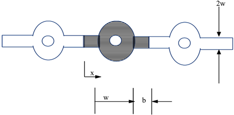
Figure 1. Schematic of fin pipe and radiative radial fin.
(4b)
A very useful parameter for fin design is the efficiency defined by the ratio of actual and ideal heat transfer rate of the fin.
(4c)
3. Elemental Discretization and Integration of the Fin Equation
A major challenge here is to create an integral analog of Equation (4a). From a theoretical viewpoint, we need a transformation that will convert our governing differential equation to an integral form that can then be resolved within a problem domain. A key feature of this approach, involves the use of the Laplacian 1-D operator as an auxiliary equation: with a fundamental solution , where represents an arbitrary constant often taken as the length of the longest element in the problem domain, and the distance between the source point and any other point is given by . Applying the Green’s identity together with the auxiliary equation to Equation (4a) and relating the whole procedure to a generic element defined by the span inside the problem domain yields
(5)
where H is the Heaviside function, and , when , for or .
We deal with the line integral in Equation (5) by approximating the dependent variable and its function with linear interpolating functions in space, i.e. where is the interpolating function and is a local coordinate for an element length . Equation (5) is the element integral analog the governing differential equation. And is solved at each node of the elementized problem domain to give the following equations at node 1 and then at node 2
(6a)
(6b)
A compact matrix representation of Equations (6a) and (6b) results in
(6c)
where the element coefficient matrices are defined as
(7a)
For the moment, it is significant to note that by discretizing the problem domain and formulating element equations, BEM integral formulation is now painlessly incorporated into an algorithm usually associated with finite element method (FEM). We now have an integral form of equation which possesses better numerical and accurate properties than its differential equivalent.
At this point, there are only two major concerns left for this hybrid formulation:
1) How to deal with nonlinearity
2) How to implement the calculations for the dependent variables with an efficient computational procedure.
Domain discretization, despite its spatial and temporal locality, has always been considered a huge disadvantage in BEM circles. Its major feature ensures that local updates of the dependent variable can be processed in contiguous elements. This allows efficient handling of the coefficient matrix as well as provide a viable numerical technique for dealing with issues related to nonlinearity, inhomogeneity, transience, and body force terms. We exploit this characteristic further by assuming that the nonlinear diffusivity is uniform within a generic element and can therefore be weight-averaged as shown.
(7b)
where and is the iteration counter. As a consequence of this approximation, and Equation (6c) now becomes
(8)
Equation (8) is still nonlinear and is handled by the Picard algorithm. where is made up of elements that depend on the solution at the previous time step. The nonlinear system of equations is solved iteratively until . The main drawback of the Picard iteration is its linear convergence rate, otherwise unlike the Newton’s technique it does not require Jacobian information.
4. Results and Discussion
The validity of the formulation developed herein was tested by comparing the numerical results with those of Torabi et al. [25] . They applied a seminumerical-analytic technique known as the differential transformation method (DTM) to calculate the temperature profile of a radiative radial fin. To justify comparison, the values chosen for their calculations are the same as those of the current study unless otherwise indicated in graphs .
Table 1 shows the closeness of the numerical and semi-analytic results. At some points, they are identical up to the fourth decimal place. This validation provides an assurance that the numerical formulation produces faithful numerical simulations where closed form or analytical results are not available.
Figure 2 shows the effect of the thermal conductivity parameter on the dimensionless temperature profile along the fin length. As increases the rate of heat transfer through the fin increases. This happens because more heat transferred by conduction through the fin increases the temperature distribution and consequently the rate of heat transfer. The effect of the internal heat generation parameter, Q on the temperature profile is depicted in Figure 3. It can be observed that an increase in Q results in a decrease of temperature gradient. This illustrates a decrease in thermal performance of the fin as the fin’s dimensionless volumetric heat generation increases. Figure 3 also suggests that at a particular limiting value of Q, the temperature profile becomes almost parallel to the non-dimensionless fin length and the temperature at the base of the fin becomes invariant with that at the tip. As a result, the conservation law supporting the formulation of the governing equation collapses and the fin becomes non-functional. It can therefore be inferred that a relatively high value of volumetric heat generation results in a situation where a greater portion of the heat generated can not escape to the environment fast enough and finally ends up in the fin surface. In this case, there is an overall gain in heat instead of heat loss. It is therefore necessary that an optimal value of Q should be known for design purposes.
Figure 4 illustrates effects of the radiation-conduction fin parameter on the scalar profile. It is observed that an increase in results in a decrease in temperature and a higher temperature gradient. An increase in signifies an increase in radiative transport. The concomitant radiative cooling sets up a higher temperature gradient around the base of the fin where a Dirichlet boundary condition exists. The overall effect is a lowering of temperature along the fin. Figure 5 displays the impact of the radiation sink temperature on the fin temperature. As can be observed, an increase in the radiative sink brings about a decrease in heat loss along the fin and a consequential rise in the temperature of the fin. In this case, the fin material acts as a sink, and further increases will eventually hinder the thermal performance of the fin.

Table 1. Comparison of numerical and analytic solutions.

Figure 2. Dimensionless temperature for various values of β.

Figure 3. Dimensionless temperature profile for various values of Q.

Figure 4. Dimensionless temperature profile for values of ψ.

Figure 5. Temperature distribution for values of θs.
Next we consider the net effect of variation on the dimensionless temperature profile along the fin length. The governing differential equation (Equation (4a)) gives us a clue. The more is increased, the less the thermal conductivity parameter plays a role in the fin’s heat transfer thermal operation. Energy conservation requires that the radiation-conduction fin parameter becomes more dominant. It can also be noted that the fin dimensionless temperature raised to the power 4 is multiplied by . This results in an overall increase in radiative transport and a consequential decrease in temperature along the fin. This is the reason why Figure 6 resembles Figure 4 but with less slope. Table 2 illustrates the effect of the variation of some fin parameters on the fin’s efficiency. For each case it can be noted that for any fixed values of and Q an increase in thermal conductivity parameter results in an increase in efficiency. This enables us to closely study the effects of variation of the dimensionless heat generation parameter together with the radiation and conduction effects on the overall fin performance. It was observed that further increase in gave physically unrealistic results. This tends to suggest that the radiation-conduction parameter must have a particular threshold value beyond which the numerical solution becomes highly unstable. We found this value to be . A similar observation under different circumstances has been made by Sobamowo [23] as well as Oguntala and Sobamowo [24] where they demonstrated the effects of thermal-geometric parameter M and internal heat generation Q on the thermal performance of a fin. They concluded that M should not exceed a certain value in order to avoid instability.
5. Conclusion
In the work reported herein a simplified, hybrid integral formulation [26] [27] has been applied to the heat transfer analysis of a radiative radial fin with a temperature dependent thermal conductivity. From the parametric studies conducted, it could be deduced that the following fin parameters namely thermal

Figure 6. Temperature distribution for values of θa.
Table 2. Fin efficiency for values of and .
conductivity, radiation-conduction fin parameter, dimensionless radiation sink parameter, volumetric heat generation all play a significant role in the fin’s energy heat transfer analysis [28] [29] . The overall temperature gradient especially noticeable near the fin base indicates an area of activity and fin performance that should play a paramount role in fin design and analysis. In fact the overall process of extracting heat from a body and dissipating it together with the internally generated heat to the ambient actually starts from there. However as observed in Figure 2 a high value of internally generated heat, gives rise to a situation where a greater portion of this energy can not escape to the ambient and the fin ends up gaining heat rather than losing it. It was also observed in Table 2, that a threshold value exits for the radiation-conduction parameter beyond which the numerical results become physically unrealistic. Hence design parameters for fin design should put these into consideration.
Conflicts of Interest
The author declares no conflicts of interest regarding the publication of this paper.
Cite this paper
Onyejekwe, O.O. (2019) Simplified Integral Calculations for Radial Fin with Temperature-Dependent Thermal Conductivity. Journal of Applied Mathematics and Physics, 7, 513-526. https://doi.org/10.4236/jamp.2019.73037
References
- 1. Kundu, B. and Das, P.K. (2007) Performance Analysis and Optimization of Elliptic Fins Circumscribing a Circular Tube. International Journal of Heat and Mass Transfer, 50, 173-180. https://doi.org/10.1016/j.ijheatmasstransfer.2006.06.043
- 2. Arslanturk, C. (2004) Performance Analysis and Optimization of a Thermally Non-Symmetric Annular Fin. International Communications in Heat and Mass Transfer, 31, 1143-1153. https://doi.org/10.1016/j.icheatmasstransfer.2004.08.012
- 3. Khani, F. and Aziz, A. (2010) Thermal Analysis of a Longitudinal Trapezoidal Fin with Temperature-Dependent Thermal Conductivity and Heat Transfer Coefficient. Nonlinear Science and Numerical Simulation, 15, 590-601. https://doi.org/10.1016/j.cnsns.2009.04.028
- 4. Hagen, K.D. (1988) Perturbation Analysis of Tapered Fins with Nonlinear Thermal Properties. Journal of Thermophysics and Heat Transfer, 2, 276-279. https://doi.org/10.2514/3.98
- 5. Mokheimer, E.M.A. (2002) Performance of Annular Fins with Different Profiles Subject to Variable Heat Transfer Coefficient. International Journal of Heat and Mass Transfer, 45, 3631-3642. https://doi.org/10.1016/S0017-9310(02)00078-9
- 6. Aziz, A. and Fang, T. (2011) Thermal Analysis of an Annular Fin with (a) Simultaneously Imposed Base Temperature and Base Heat Flux and (b) Fixed Base and Tip Temperatures. Energy Conversion Management, 52, 2467-2478. https://doi.org/10.1016/j.enconman.2011.02.004
- 7. Khou, H.S., Lee, J.J. and Lai, C.Y. (2005) Thermal Analysis of a Longitudinal Fin with Variable thermal Properties by Recursive Formulation. International Journal of Heat and Mass Transfer, 48, 2266-2277. https://doi.org/10.1016/j.ijheatmasstransfer.2004.12.038
- 8. Campoa, A. and Chikhb, S. (2006) Reproduction of Fin Efficiency Diagram for Annular Fins of Uniform Thickness by Solving Systems of Four Algebraic Equations. International Journal of Mechanical Engineering Education, 34, 85-92. https://doi.org/10.7227/IJMEE.34.1.7
- 9. Lesnic, D. and Heggs, P.J. (2004) A Decomposition Method for power-Law Fin-Type Problems. International Communications in Heat and Mass Transfer, 31 673-682. https://doi.org/10.1016/S0735-1933(04)00054-5
- 10. Khan, W.A. and Aziz, A. (2012) Transient Heat Transfer in a Heat-Generating Fin with Radiation and Convection with Temperature-Dependent Heat Transfer Coefficient. Heat Transfer-Asian-Research, 41, 402-417. https://doi.org/10.1002/htj.21012
- 11. Kraus, A. and Aziz, A.J. (2001) Welty Extended Surface Heat Transfer. John Wiley and Sons, New York.
- 12. Moitsheki, R.J. and Harley, C. (2011) Transient Heat Transfer in Longitudinal Fins of Various Profiles with Temperature-Dependent Thermal Conductivity and Heat Transfer Coefficient. Pramana—Journal of Physics, 77, 519-532. https://doi.org/10.1007/s12043-011-0172-6
- 13. Rusagara, I. and Harley, C. (2013) A Numerical Well-Balanced Scheme for One-Dimensional Heat Transfer in Longitudinal Triangular Fin. Mathematical Problems in Engineering, 2013, Article ID: 609536. https://doi.org/10.1155/2013/609536
- 14. Yaghoobi, H. and Torabi, M. (2011) The Application of Differential Transformation Method to Nonlinear Equations Arising in Heat Transfer. International Communications in Heat and Mass Transfer, 38, 815-820. https://doi.org/10.1016/j.icheatmasstransfer.2011.03.025
- 15. Moitsheki, R.J. (2011) Steady Heat Transfer through a Radial Fin with Rectangular and Hyperbolic Profiles. Nonlinear Analysis: Real World Applications, 12, 867-874. https://doi.org/10.1016/j.nonrwa.2010.08.011
- 16. Arslanturk, C. (2006) Optimal Design of Space Radiators with Temperature Dependent Thermal Conductivity. Applied Thermal Engineering, 26, 1149-1157. https://doi.org/10.1016/j.applthermaleng.2005.10.038
- 17. Atay, M.T. and Coskun, S.B. (2008) Comparative Analysis of Power-Law Fin-Type Problems Using Variational Iteration Method and Finite Element Method. Mathematical Problems in Engineering, 2008, Article ID: 635231. https://doi.org/10.1155/2008/635231
- 18. Aziz, A. and Enamul-Huq, S.M. (1973) Perturbation Solution for Convective Fin with Internal Heat Generation and Temperature Dependent Thermal Conductivity. International Journal of Heat and Mass Transfer, 97, 300-301.
- 19. Aziz, A. (1977) Perturbation Solution for Convective Fin with Internal Heat Generation and Temperature Dependent Thermal Conductivity. International Journal of Heat and Mass Transfer, 20, 1253-1255. https://doi.org/10.1016/0017-9310(77)90135-1
- 20. Poozesh, S., Nabi, S., Saber, M., Dinarv, S. and Fani, B. (2012) The Efficiency of Convective-Radiative Fin with Temperature-Dependent Thermal Conductivity by the Differential Transformation Method. Research Journal of Applied Sciences, Engineering and Technology, 6, 1354-1359.
- 21. Hassanzadeh, R. and Pekel, H. (2013) Heat Transfer Enhancement in Annular Fins Using Functionally Graded Material. Heat Trans-Asian Research, 42, 603-617. https://doi.org/10.1002/htj.21053
- 22. Jain, M.K., Iyenger, K. and Jain, R.K. (2010) Numerical Methods for Scientific and Engineering Computation. 5th Edition, New Age Int. Ltd.
- 23. Sobamowo, M.G. (2016) Analysis of Convective Longitudinal Fin with Temperature-Dependent Thermal Conductivity and Internal Heat Generation. Alexandria Engineering Journal, 56, 1-11. https://doi.org/10.1016/j.aej.2016.04.022
- 24. Oguntala, M.K.G. and Sobamowo, M.G. (2016) Galerkin’s Method of Weighted Residual for a Convective Straight Fin with Temperature Dependent Conductivity. International Journal of Engineering and Technology, 12, 432-442.
- 25. Torabi, M., Yaghoobi, H., Colantoni, A., Biondi, P. and Boubaker, K. (2016) Analysis of Radiative Radial Fin with Temperature-Dependent Thermal Conductivity Using Nonlinear Transformation Methods. Chinese Journal of Engineering, 2016, Article ID: 470696. https://doi.org/10.1155/2013/470696
- 26. Onyejekwe, O.O. (2016) Localized Boundary-Domain Integro-Partial Differential Formulations for Transient Scalar Transport Problems. International Journal of Applied and Computational Mathematics, 3, 2189-2204.
- 27. Onyejekwe, O.O. (2017) Element Localized Boundary Integral Formulation for Transient Nonlinear Problems. International Journal of Nonlinear Science, 24, 67-75.
- 28. Deka, A. and Datta, D. (2019) Multiobjective Optimization of Annular Fin Array Subject to Thermal Load. Journal of Thermophysics and Heat Transfer, 33, 254-263. https://doi.org/10.2514/1.T5394
- 29. Das, R. and Kundu, B. (2018) Prediction of Heat Generation in a Porous Fin from Surface Temperature Journal of Thermophysics and Heat Transfer, 4, 781-790.