Journal of Applied Mathematics and Physics
Vol.03 No.06(2015), Article ID:57407,8 pages
10.4236/jamp.2015.36079
Estimate Beta Coefficient of CAPM Based on a Fuzzy Regression with Interactive Coefficients
Yalei Du, Qiujun Lu
College of Science, University of Shanghai for Science and Technology, Shanghai, China
Email: yaleidu@163.com, fuzzy_lu@163.com
Copyright © 2015 by authors and Scientific Research Publishing Inc.
This work is licensed under the Creative Commons Attribution International License (CC BY).
http://creativecommons.org/licenses/by/4.0/


Received 16 April 2015; accepted 21 June 2015; published 25 June 2015
ABSTRACT
In the Capital Asset Pricing Model (CAPM), beta coefficient is a very important parameter to be estimated. The most commonly used estimating methods are the Ordinary Least Squares (OLS) and some Robust Regression Techniques (RRT). However, these traditional methods make strong as sumptions which are unrealistic. In addition, The OLS method is very sensitive to extreme observations, while the RRT methods try to decrease the weights of the extreme observations which may contain substantial information. In this paper, a novel fuzzy regression method is proposed, which makes less assumptions and takes good care of the extreme observations. Simulation study and real word applications show that the fuzzy regression is a competitive method.
Keywords:
CAPM, Beta Coefficient, Fuzzy Regression, Outlier

1. Introduction
The evaluation of risky asset has always been a hot topic in finance. [1] proposed that the risk of an asset can be measured as variance. Furthermore, the total variance of an asset contains two parts: systematic risk and unsystematic risk. According to the Capital Asset Pricing Model (CAPM), the systematic risk is measured as the beta coefficient, which is defined as the expected change of an asset for every percentage change in the benchmark index [2] . The beta coefficient is generally estimated by the following regression model:
 (1)
(1)
 refers to the return of asset i;
  refers to the return of the market;
  is a constant term;
  is the sensitivity of the return of asset i to the return of the market;
 ![]() is the random effect that can not be explained.
is the random effect that can not be explained.
A high value of ![]() means a riskier asset, while a small
means a riskier asset, while a small ![]() refers a more secure asset. The goal of CAPM is to estimate the coefficients
refers a more secure asset. The goal of CAPM is to estimate the coefficients ![]() and
and ![]() given the market return
given the market return ![]() and the asset return
and the asset return ![]() as input and out- put respectively.
as input and out- put respectively.
The most commonly used estimating technology is the OLS method. But OLS is very sensitive to extreme observations, which means an outlier may cause a large effect on the estimation. Since the market is complex and volatile, the estimation of OLS is not robust, hence OLS is inappropriate to estimate the beta coefficient.
To decrease the effects of extreme observations, some robust regression techniques (RRT) are proposed. During the RRT methods, Huber and Bi-square estimations are the most commonly used methods. These methods employ an algorithm called Iteratively Re-weighted least squares (IRLS) to compute the estimation. The algorithm tries to minimize a weighted square of error in which the weights of outliers will be decreased [3] . However, it is common to see extreme observations in the financial markets, and they may carry substantial information which can help investors make risky investment decisions to boot their profits.
On the other hand, RRT methods also ignore the probability imprecision of the data. In these cases, fuzzy regression methods are alternative choices. The fuzzy regression was first proposed by [4] , in which the input and output are crisp and fuzzy number respectively, and the estimation was solved as a linear programming system. The membership function (msf) of the fuzzy set is often described as possibility distribution, so fuzzy regression is also called possibilistic regression analysis [5] - [8] . Another approach of fuzzy regression is the fuzzy least squares, which is proposed by [9] [10] . [11] proposed fuzzy least squares regression for crisp inputs and fuzzy output. [5] formalized possibility regression with quadratic membership functions, which can deal with interactive possibility distributions, hence obtain interactive coefficients. Furthermore, [6] proposed possibility regression based on exponential possibility distributions, which is called exponential possibility regression. Due to the shortcoming of their algorithm, the center values and the possibility distribution are estimated separately.
The rest of the paper is organized as follows. The exponential possibility regression proposed by [6] is introduced in Section 2. Then an improved model with a new algorithm is proposed, and a small case shows its better performance. Section 3 compares the results of new fuzzy regression model with OLS and RRT methods using simulated data. At last two real world applications is implemented in Section 4 to test the performance of fuzzy regression.
2. Fuzzy Regression Model with Interactive Coefficients
2.1. Exponential Possibility Regression
The exponential possibility regression proposed by [6] is defined as:
![]() (2)
(2)
where ![]() is the input vector of ith sample, an s is a constant 1.
is the input vector of ith sample, an s is a constant 1. ![]() is the
is the
fuzzy coefficients vector, which is defined by the following exponential possibility distribution with a center vector c and a symmetrical positive definite matrix D:
 (3)
(3)
where A = (a, D). As a result, the possibility distribution of the output is
 (4)
(4)
It is also called the membership function of y.  and
and  are the center and spread of y respectively. The spread can also be interpreted as statistical errors in statistical regression analysis. The way of estimating is minimizing the spread subject to the level constraints:
 (5)
(5)
In Equation (5), D > 0 is a non-linear constraint. [6] uses a two-step estimation strategy, in which the first step determines the center vector a using the interval regression or the ordinary least squares regression, then the second step substitutes the obtained center vector  into the constraints in Equation (5).
In the second step, to overcome the non-linear constraint D > 0, [6] use an orthogonal condition  (for all
 ) instead. It has been proved that the orthogonal condition ensures D can be obtained as a positive definite matrix if
  are independent.
2.2. Update Algorithm
However, the constraint  (for all
 ) is an unnecessary and sufficient condition of D > 0. Theso- lution of [6] may not be the optimal one.
Actually, Equation (5) can be converted to a semidefinite programming (SDP) problem, which can be solved by many softwares now (for example [12] ). While solving the problem, the matrix D is consider as a positive semi definite matrix. After done, if the determinant of D equals to 0, say , an extra ridge down the diagonal will be added, i.e.
  where
where  is a small positive number and I is a identity matrix. This trick is inspired by the ridge regression.
In addition, the center vector a and matrix D can be solved at the same time, there is no need to makea two-step estimation.
We implement our new algorithm on a numerical example in [6] , the data is shown in Table 1.
The original optimal value in [6] is 86.13. The solution of new algorithm before adding a scalar matrix is 62.72, which is much smaller than the original solution. To solve it, we used CVX, a package for specifying and solving convex programs [12] [13] . Here is the code:
x = [2, 4, 6, 9, 12, 13, 14, 16, 29, 20];
x = [ones(10, 1), x’];
y = [4, 7, 5, 8, 7, 9, 12, 9, 14, 10];
m, n = size(x)
cvx_begin
varable a(n);
variable D(n,n) symmetric;
D == semidefinite (n);
minimize (sum( diag (x * D * x')))
subject to
diag (x * D * x ') >= (y − x*a). ^2/(−log (0.5))
cvx _end
However, the estimated matrix  is nearly a positive semidefinite matrix (
 ,). So a scalar matrix
  is added. The code “D == semidefinite(n)” is replaced with “D = semidefinite(n) + 0.01*diag (diag(ones(2)))”.
Then the matrix D is:

And the optimal value here is 65.37, which is also much smaller than the original solution 86.13. It showsthat by using the modern algorithm and software, the new estimation is much better than the old one.

Table 1. Input-output data of the numerical example.
2.3. Update Model
In [6] , the parameter h-cut level is chosen manually as 0.5. However, there are couples of arguments about the h- cut level. [8] [14] proposed that h-level should be 0.5 and 0.9 respectively. There are also several theories argue that h should be 1.
To overcome the h-cut level problem, [15] use the inequality  to replace the h-cut constraints.
  and
and  are estimated msf and observed msf of y respectively.
  means that the membership values of the estimated output are taken equal or larger than the membership degree of the observed output. If
  is taken, the inequality can be simplified as:
 (6)
(6)

In this study, we also use the inequality  constraints, and
  is chosen by the msf of output
 (7)
(7)
In cases of , we have
 . Since the expression
  is non- negative,
  , results into
 , which is equivalent to
  If more than
two points has log , it’s unlikely to find a line going through all these samples. Constraints like this are very likely to make the problem infeasible to solve.
Inspired by the Support Vector Machine (SVM) [16] , which adds a extra parameter  so that the model can tolerate some misclassification samples.

We add another parameters  to extend the constraints. Furthermore, in this study, the squared error is added in the objective function to get a better fitting. Here is the final model:
 (8)
(8)
It is equivalent to the following programming problem:
 (9)
(9)
C is a parameter determined manually, which is used to balance the influence of the sum of squared errors and the sum of spreads, as well as the effects of outliers (sum of ).
).
3. Simulation Study
In this Section, we try to use the simulated data to test the fuzzy regression model.
The simulated data here is generated by the formula  where
where  and
and . Anyone can run the following codes in R [17] to reproduce the data.
set.seed(0)
x = rnorm(30 , 0 , sd = 0.1)
y = 1.2 * x − 0.0 2 + rnorm(30, 0, sd = 0.05)
y[27] = y [27] + 0.4
The codes generate 30 observations and add 0.4 to the outcome of 27th observation to make a faked outlier.
To estimate the beta coefficient, four methods were used. As we can see in Table 2, all the beta coefficients are significantly meaningful at the 5% significance level. Compare the beta coefficients of these methods, Huber estimation is the most accuracy one in this case, and the Fuzzy method takes the second place.
According to Figure 1, there are two outliers. The first one has Cook’s distance of 0.85, and the second one is 0.14. The second outlier may contain substantial information, so that we should pay more attention to it. In this simulation, we know that the first outlier is a true outlier and the second is a faked one.
The regression line of OLS method is sensitive to the outlier with high Cook’s distance, while the RRT methods are not sensitive to outliers, since they decrease the weights of outliers. The fuzzy regression line is also robust. Compared with the OLS regression line, the fuzzy regression line tends to make a movement in direction of the outlier with lower Cook’s distance.
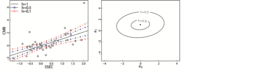
Furthermore, the optimal matrix D in this case is , which is nearly a positive semidefinite matrix (
 ). The possibility regression model and possibility distribution of coefficients are shown in Figure 2.
Since the matrix D is positive semidefinite, we add it up to a scalar matrix to make it positive definite. Then the solution is . Now the eigen values of D are 0.22 and 0.01, which means D is a positive definite matrix.
Thus, the possibility regression model and possibility distribution of coefficients become to Figure 3.
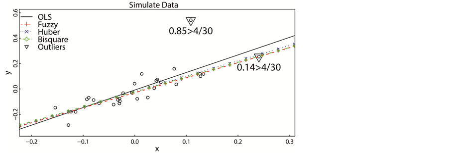
Figure 1. Regression analysis of simulated data.
Table 2. Analysis of simulated data.
 (a) (b)
Figure 2. The possibility regression model and possibility distribution of coefficients. (a) Possibility regression model; (b) possibility distribution of coefficients.
 (a) (b)
Figure 3. The possibility regression model and possibility distribution of coefficients after adding a scalarmatrix. (a) Possibility regression model; (b) possibility distribution of coefficients.
4. Real World Applications
In this Section, the data sets of assets of China Northern Rare Earth (CNRE, SSE number: 600111) and China Merchants Bank (CMB, SSE number: 600036) traded at the Shanghai Stock Exchange and the Shanghai Stock Exchange Composite (SSEC) Index are used. The sample data contains the return of these three assets per day in October and November 2014, and the return is calculated by the formula:

where Popen refers to the opening price,  refers to the closing price.
To check the existence of extreme samples, we employ the Cook’s distance. According to the Cook’s distance criterion, the samples with Cook’s distance greater than 4/n are regarded as extreme observations.
In the procedure of estimating the beta coefficient, OLS method and RRT methods are used, as well as our fuzzy method.
4.1. Regression Analysis of CMB
In this first case, the price of stock of CMB (600036) and the SSE Composite Index (SSEC) are used. We employ the Cook’s distance to check the existence of extreme observations.
According to Figure 4, three extreme observations are determined. The Cook’s distance of the first outlier is 0.17, and the second one is 0.12 while the third one is 1.3 which is extremely large. The first two outliers may contain substantial information, so that we should pay more attention to them.
As we can see in Table 3, all the beta coefficients are significantly meaningful at the 5% significance level. The beta coefficients of Bisquare and Huber methods are smaller than 1, while the beta coefficients of OLS and Fuzzy methods are greater than 1.

Figure 4. Regression analysis of CMB.
Table 3. Analysis of CMB.
In Figure 4, the regression Fuzzy method is between the regression lines of OLS method and RRT methods. Since the regression line of OLS is very sensitive to the outlier with Cook’s distance of 1.3, while the RRT me- thods tends to ignore the influence of the outlier with the largest Cook’s distance. The fuzzy regression is the mildly sensitive to the outliers, it is resistant to extreme observations with very large Cook’s distance, while it also takes care of the extreme observations with smaller Cook’s distance. Figure 5 shows the possibility regression model and possibility distribution of estimated coefficients.
4.2. Regression Analysis of CNRE
In the second case, the price of stock of CNRE (600111) and the SSE Composite Index (SSEC) are used. According to Figure 6, two extreme observations are determined. The first one has Cook’s distance of 0.25, and the second one is 0.52, both of them are not very large, so they may contain substantial information, and we should pay attention to them.
As Table 4 shown, all the beta coefficients are significantly meaningful at the 5% significance level.
The Huber and Bisquare methods are not sensitive to outliers, even outliers with not so large Cook’s distance. While OLS method is very sensitive to outliers, and the Fuzzy method takes care of outliers with “faked” outliers. As a result, the beta coefficients of Bisquare and Huber are greater than 1, while the beta coefficients of OLS and Fuzzy methods are smaller than 1.
5. Conclusions
According to the simulation study and real world applications, we can see that our new fuzzy regression model with modern computation algorithm has a good performance. The traditional ordinary least squares regression is too sensitive to the outliers, while the RRT methods are very robust so that they may ignore the influence of faked outliers (outliers with small Cook’s distances). However, due to the vary of the finance market, some normal observations may be treated as outliers. The Cook’s distances of these observations may be slightly larger than 4 = n and we should pay more attention to them.
The fuzzy regression method tends to take into account the extreme observations with smaller Cook’s distance, while it is also insensitive to the extreme observations with large Cook’s distance.
 (a) (b)
Figure 5. The possibility regression model and possibility distribution of coefficients of CMB. (a) Possibility regression model; (b) possibility distribution of coefficients.

Figure 6. Regression analysis of CNRE.
Table 4. Analysis of CNRE.
In conclusion, our new fuzzy regression may be a better choice for estimating the beta coefficient. More generally, it is a good tool for observations with outliers.
Fund
Hujiang Foundation of China (B14005); Startup Foundation project for doctor of USST (100034100).
References
- Markowitz, H. (1952) Portfolio Selection. The Journal of Finance, 7, 77-91.
- Clarfeld, R.A. and Bernstein, P. (1997) Understanding Risk in Mutual Fund Selection. Journal of Accountancy, 184, 45-49.
- Holland, P.W. and Welsch, R.E. (1977) Robust Regression Using Iteratively Reweighted Least-Squares. Communi-Cations in Statistics-Theory and Methods, 6, 813-827. http://dx.doi.org/10.1080/03610927708827533
- Tanaka, H. and Asai, K. (1984) Fuzzy Linear Programming Problems with Fuzzy Numbers. Fuzzy Sets and Systems, 13, 1-10. http://dx.doi.org/10.1016/0165-0114(84)90022-8
- Tanaka, H. and Ishibuchi, H. (1991) Identification of Possibilistic Linear Systems by Quadratic Membership Functions of Fuzzy Parameters. Fuzzy Sets and Systems, 41, 145-160. http://dx.doi.org/10.1016/0165-0114(91)90218-F
- Tanaka, H., Ishibuchi, H. and Yoshikawa, S. (1995) Exponential Possibility Regression Analysis. Fuzzy Sets and Systems, 69, 305-318. http://dx.doi.org/10.1016/0165-0114(94)00179-B
- Tanaka, H. and Lee, H. (1998) Interval Regression Analysis by Quadratic Programming Approach. IEEE Transactions on Fuzzy Systems, 6, 473-481. http://dx.doi.org/10.1109/91.728436
- Tanaka, H., Uejima, S. and Asai, K. (1982) Linear Regression Analysis with Fuzzy Model. IEEE Transactions on Systems, Man and Cybernetics, 12, 903-907. http://dx.doi.org/10.1109/TSMC.1982.4308925
- Celmi, A. (1987) Least Squares Model Fitting to Fuzzy Vector Data. Fuzzy Sets and Systems, 22, 245-269. http://dx.doi.org/10.1016/0165-0114(87)90070-4
- Celmi, A. (1987) Multidimensional Least-Squares Fitting of Fuzzy Models. Mathematical Modelling, 9, 669-690. http://dx.doi.org/10.1016/0270-0255(87)90468-4
- Diamond, P. (1988) Fuzzy Least Squares. Information Sciences, 46, 141-157. http://dx.doi.org/10.1016/0020-0255(88)90047-3
- Michael, G. and Stephen, B. (2013) CVX: Matlab Software for Disciplined Convex Programming, Version 2.0 Beta. http://cvxr.com/cvx
- Michael, G. and Stephen, B. (2008) Graph Implementations for Nonsmooth Convex Programs. Springer-Verlag Limited, 95-100.
- Civanlar, M.R. and Trussell, H.J. (1986) Constructing Membership Functions Using Statistical Data. Fuzzy Sets and Systems, 18, 1-13.
- Kocadagli, O. (2013) A Novel Nonlinear Programming Approach for Estimating CAPM Beta of an Asset Using Fuzzy Regression. Expert Systems with Applications, 40, 858-865. http://dx.doi.org/10.1016/j.eswa.2012.05.041
- Suykens, J.A. and Vandewalle, J. (1999) Least Squares Support Vector Machine Classifiers. Neural Processing Letters, 9, 293-300. http://dx.doi.org/10.1023/A:1018628609742
- R Core Team (2014) R: A Language and Environment for Statistical. http://www.R-project.org