ABSTRACT

We are interested in the coexistence of three species forming a tritrophic food chain model. Considering a linear grow for the lowest trophic species or prey, and a type III Holling functional response for the middle and highest trophic species (first and second predator respectively). We prove that this model exhibits two small amplitud periodic solutions bifurcating simultaneously each one from one of the two zero-Hopf equilibrium points that the model has adequate values of its parameters. As far as we know, this is the first time that the phenomena appear in the literature related with food chain models.

1. Introduction

In general, the Hopf bifurcation is a useful tool to analyse the existence of limit cycles in predator-prey interaction models. For instance, in [1] the authors proved the existence, uniqueness and nonexistence of limit cycles in a predator-prey model considering a strong Allee effect in a prey. In [2], it is considered that a model of three species competes for three resources and it is proved that the existence of two limit cycles evolves the coexistence equilibrium point, and other example is [3]. In a food web the Hopf bifurcation is also the principal tool for proving the coexistence of species that compose the food chain. In this direction Freedman and Waltman [4] studied the persistence of species in a three-level food chain model. They introduce a relative general model, and criteria for the boundedness and stability are established. They consider a Lotka-Volterra predation with a carrying capacity at the lowest level via a logistic map and with a Holling functional response type II predation at the level of the first predator. They gave sufficient conditions for persistence of all three species. Later on, in [5] Freedman and So established criteria for which a simple food-chain model had a globally stable positive equilibrium and also developed criteria in order that such a food chain model exhibited uniform persistence (see also [6]). In these articles, the possibility of existence of limit cycles is important, however it was not studied.

Recently Françoise and Llibre analyse a model representing a tritrophic food chain composed of a logistic prey, a Holling type II predator and a Holling type II toppredator in [7]. Using the averaging theory (see [8-10]) they prove the existence of a stable periodic orbit contained in the region of coexistence of the three species in a tritrophic chain. For some values of the parameters three limit cycles born via a triple Hopf bifurcation. One is contained in the plane where the top-predator is absent. Another one is not contained in the domain of interest where all variables are positive and the third one is contained where the three species coexist. In the literature, there are many papers dedicated to find these types of limit cycles which came from a Hopf bifurcation, but in all these papers the existence of a triple Hopf bifurcation was not proved analytically, see for instance [11-16].

In this paper we analyse a tritrophic food chain model considering Holling functional response of type III for middle and top trophic level and linear grow for the lowest tropic level.

Accordingly with the previous works a general tritrophic food chain model has the form

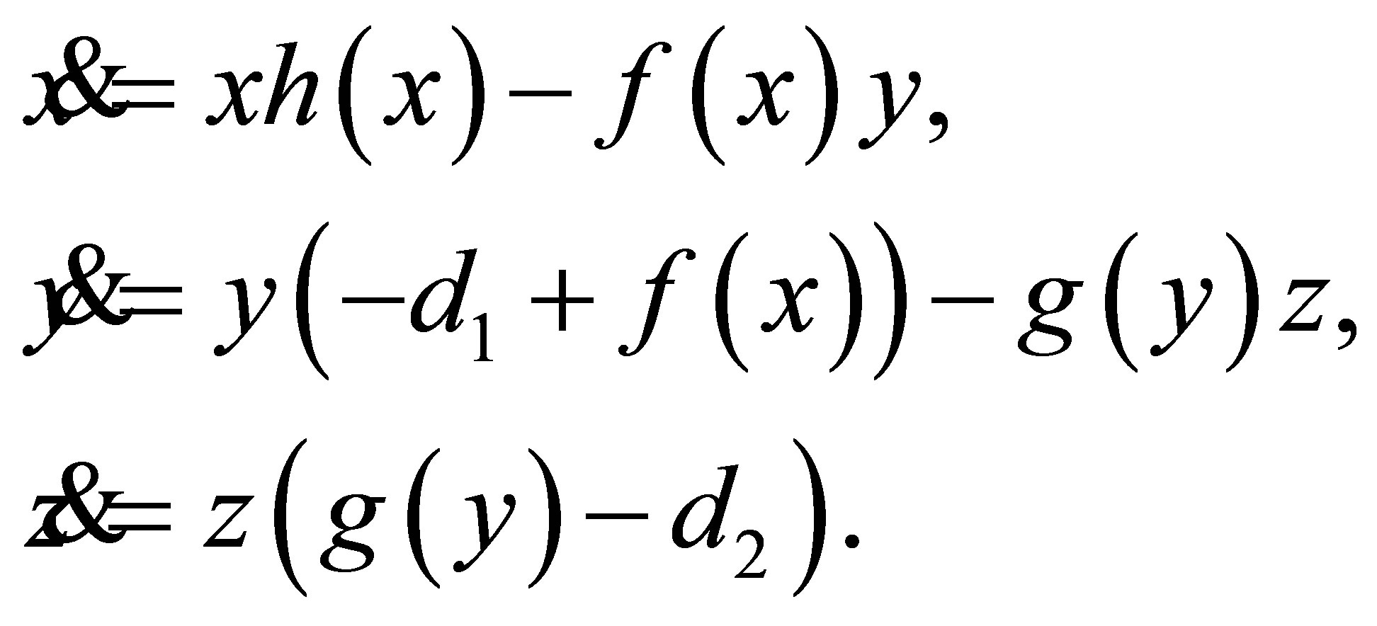
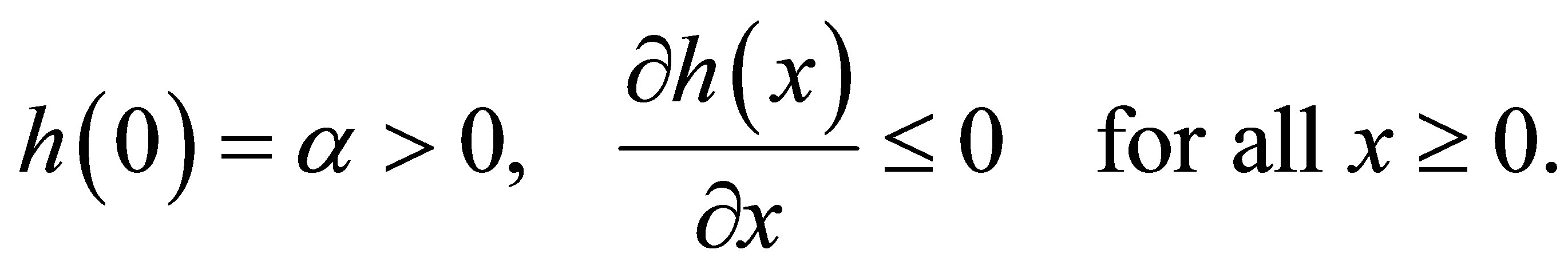
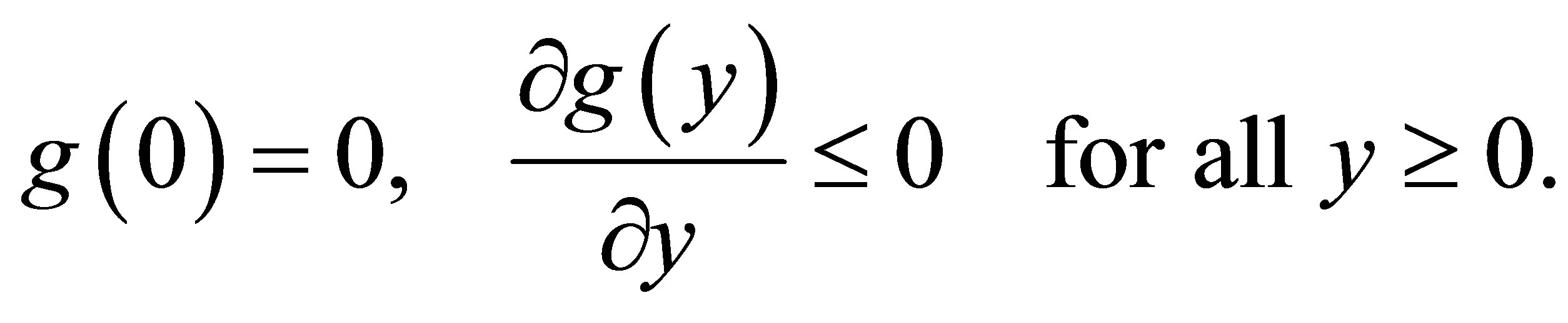
here x represents the number of lowest trophic species or prey, y is the number of the middle trophic level species or first predator (called also as predator), and z is the number of highest trophic level species or second predator (super-predator). The parameters a₁ and d₂ are positives. The function 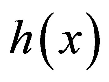represents the specific growth rate of the prey and must always satisfy

The function is the functional response of predator (second consumer or first predator) and must satisfy

Finally, the function 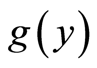is the functional response of the super-predator (tertiary consumer or second predator) and satisfies the conditions

There are many functions that satisfy the above conditions, for example the functional responses of predation include the usual functions found in the literature (see, e.g., [17]). In this paper we will consider linear growth without environmental carrying capacity for the prey and Holling functional response type III for the predator and the super-predator. So we consider the functions

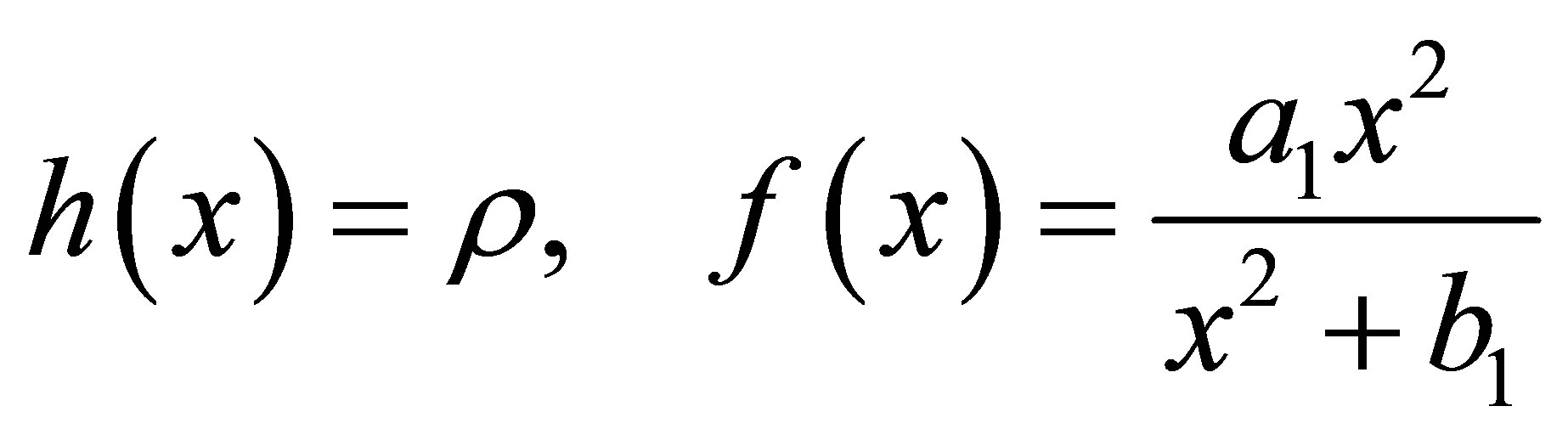
where and are positive constants. Consequently, the tritrophic food chain model that we shall study is

(1)

For ecological restrictions the analysis is in the positive octant of, i.e. in the region, and.

We give necessary conditions on the parameters to guarantee the existence of two equilibrium points of the differential System (1) in the region of interest. At these equilibrium points we find two families of parameters for which these equilibrium are zero-Hopf, see Proposition 1. The main result shows that only one of these families of parameters produces a double simultaneously zero-Hopf bifurcation, appearing at the same time two small amplitude periodic orbits bifurcating simultaneous of the two different equilibria of the system, see Theorem 2.

2. Equilibrium Points in the Positive Octant

As we mention above, the tritrophic food chain model (1) has two equilibrium points in the positive octant of 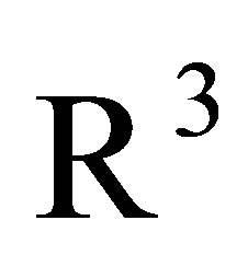when the parameters satisfy the following three conditions:

1)

2)

3)

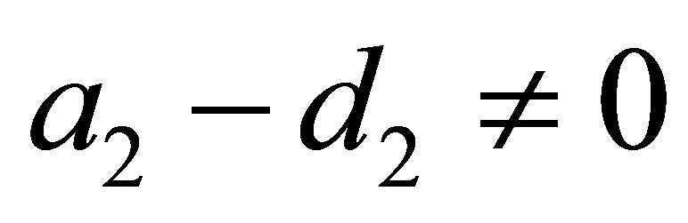
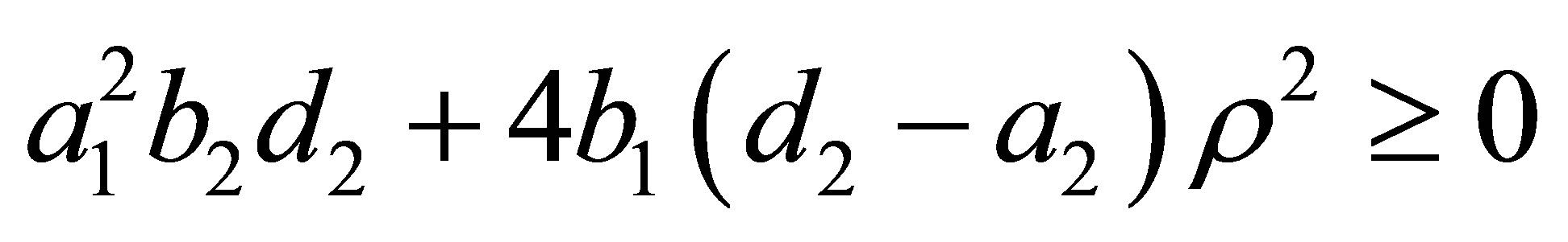
These conditions are necessary because in the coordinates of these two equilibrium points appear the expression

In order that the expression of the equilibrium points become easier we change the parameter for the new parameter defined through

Solving in terms of from the above expression we obtain

Therefore we need that, otherwise would be negative. Hence the Condition (i) becomes

. (i)

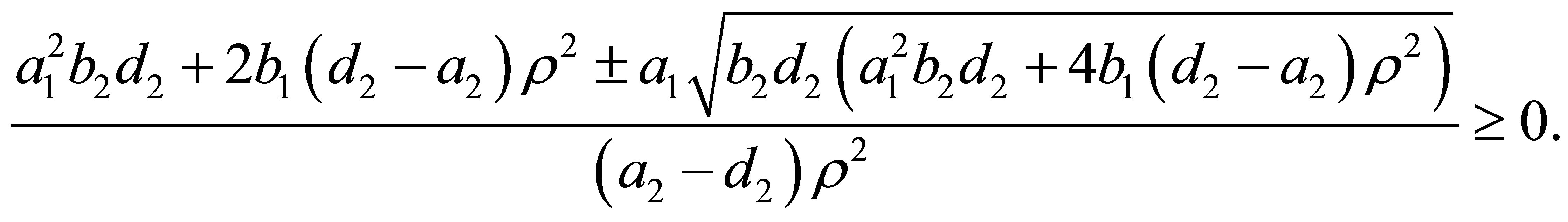
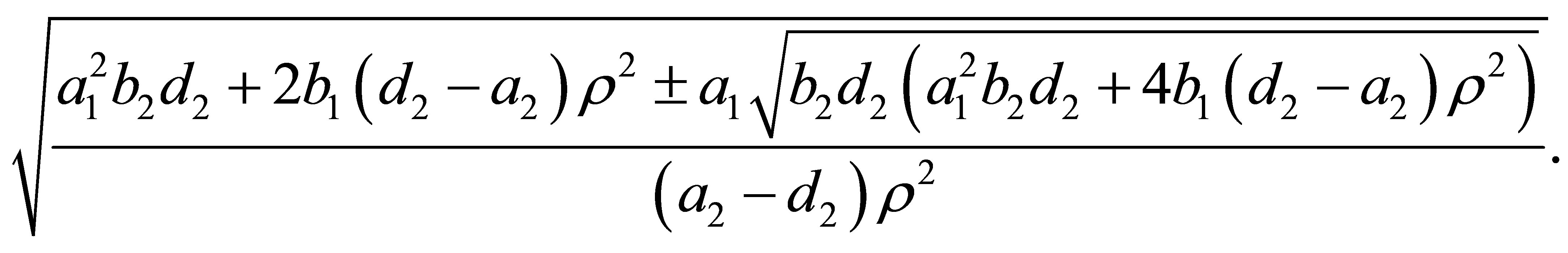
Now equating system (1) to zero and solving it we obtain two equilibrium points in the positive octant, which are

Our first interest is to analyse when of these two equilibrium points are of type zero-Hopf.

3. Zero-Hopf Equilibrium Points and Bifurcation

We recall that an equilibrium point is a zero-Hopf equilibrium of a 3-dimensional autonomous differential equation, if it has a zero real eigenvalue and a pair of purely imaginary eigenvalues. We know that a zero-Hopf bifurcation is a two-parameter unfolding (or family) of a 3- dimensional autonomous differential system with a zeroHopf equilibrium. The unfolding has an isolated equilibrium point with a zero eigenvalue and a pair of purely imaginary eigenvalues if the two parameters take zero values, and the unfolding has different topological type of dynamics in the small neighbourhood of this isolated equilibrium as the two parameters vary in a small neighbourhood of the origin. This theory of zero-Hopf bifurcation has been analysed by Guckenheimer, Han, Holmes, Kuznetsov, Marsden and Scheurle in [18-22]. In particular it is shown that some complicated invariant sets of the unfolding could bifurcate from the isolated zero-Hopf equilibrium under some conditions. Hence in some cases the zero-Hopf bifurcation could imply a local birth of “chaos” see for instance the articles [22-26] of Baldomá and Seara, Broer and Vegter, Champneys and Kirk, Scheurle and Marsden.

In the next result we characterize when the equilibrium points or of our tritrophic system (1) are zeroHopf equilibrium.

Proposition 1 The equilibrium points and are zero-Hopf equilibrium points simultaneously if and one of the following two conditions holds:

1) and.

2).

Proof. The proof is made computing directly the eigenvalues at each equilibrium point. First, the characteristic polynomial of the linear approximation of the tritropic system (1) at the equilibrium is

where,

Imposing the condition that , we obtain a system of three equations, that correspond to the coefficients of the terms of degree 0, 1 and 2 in of the polynomial. So the solutions of this system in terms of the variables and are the next three group of solutions:

(s1)

(s2)

(s3)

Here each for is a funciton in the parameters of the system that it is not necessary to provide explicitly. We must omit solution (s2) because it does not satisfy condition (i).

As we want that the eigenvalues of the linear approximation at are 0 and, we need that to conclude that is a zero-Hopf equilibrium point.

1) When is zero we have two cases for (s1).

a) and. Then we have that the eigenvalues are 0 and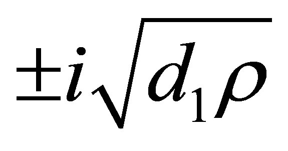. Then is a zero-Hopf equilibrium. This corresponds to statement (b) for.

b) and. In this case the eigenvalues are 0 and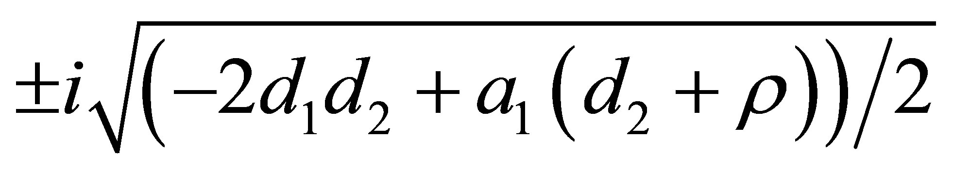. So in order to obtain purely imaginary conjugate eigenvalues it is necessary that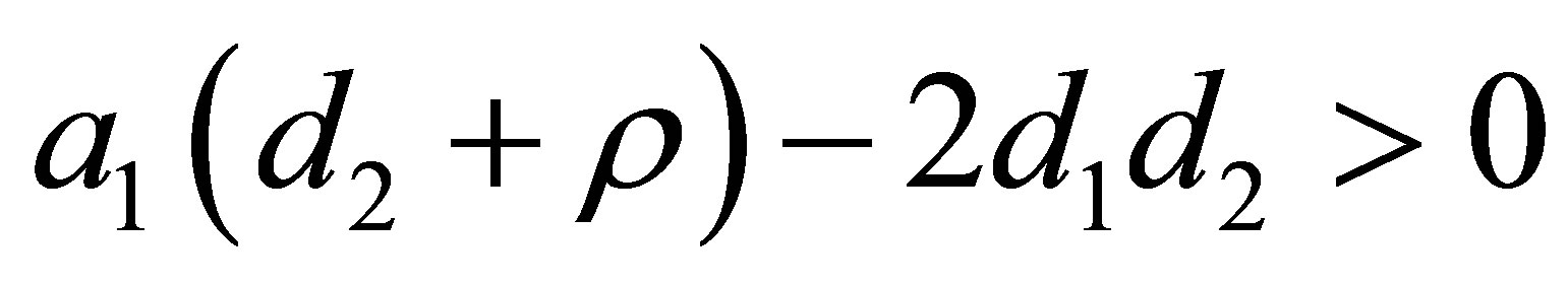. Then is a zero-Hopf equilibrium. This corresponds to statement (a) for.

2) In (s3) we have that if and only if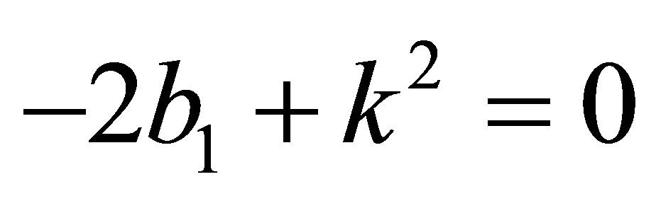, which implies that. So the eigenvalues at the point are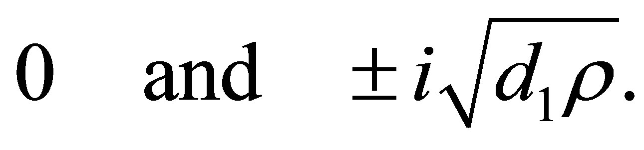

Then we have two pure imaginary conjugate eigenvalues and then is zero-Hopf equilibrium. Since we again obtain statement (b) for.

In a similar way we study the eigenvalues of the linear approximation at the equilibrium point to complete the proof of the proposition. Thus, the set of solutions of the corresponding system of equations determined from the coefficients of degree 0, 1 and 2 in of the equality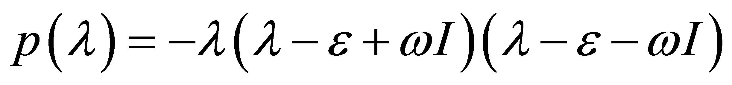, where 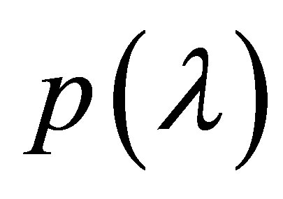is the characteristic polynomial of the linear part at the point, in terms of variables and, are

(s4)

(s5)

(s6)

Also here each for has an expression in function of the parameters that it is not necessary to write. Again we must omit the solution (s5) because it does not satisfy condition (i).

If we made the analysis using the set of solutions (s4) and (s6), we obtain again the statements (a) and (b) for the equilibrium point. This completes the proof of the proposition.

4. The Main Result

Proposition 1 guarantees the existence of three-dimensional parameter families for which the equilibrium points and are of zero-Hopf type simultaneously. Therefore it is possible to have simultaneously two zeroHopf bifurcations, one on each equilibrium. The following theorem establishes that one of these two families of parameters gives rise to a simultaneously zero-Hopf bifurcation in each equilibria, in the sense that a small amplitude periodic orbit borns simultaneously at and. For the other family of simultaneous zero-Hopf equilibria it is not possible, using the averaging theory, to show that small amplitude periodic orbits borns from those equilibria simultaneously.

Theorem 2 Assume that the parameters satisfy:

1)

2) where is a small parameter

3), and

4).

Then for sufficiently small two small amplitude periodic orbits born simultaneously one at the equilibrium point and the other at the equilibrium point when.

Proof. We prove this theorem using the averaging theory of first order, a summary of this theory is given in the appendix. This summary facilitates to follow the computations necessary for proving this theorem.

The hypotheses of the theorem imply that the equilibrium points and are zero-Hopf when (see statement (a) of Proposition 1). First, we prove that at the point there is a zero-Hopf bifurcation. We translate the equilibrium point to the origin of coordinates and we substitute and with a small paramete. Then the differential system (1) becomes

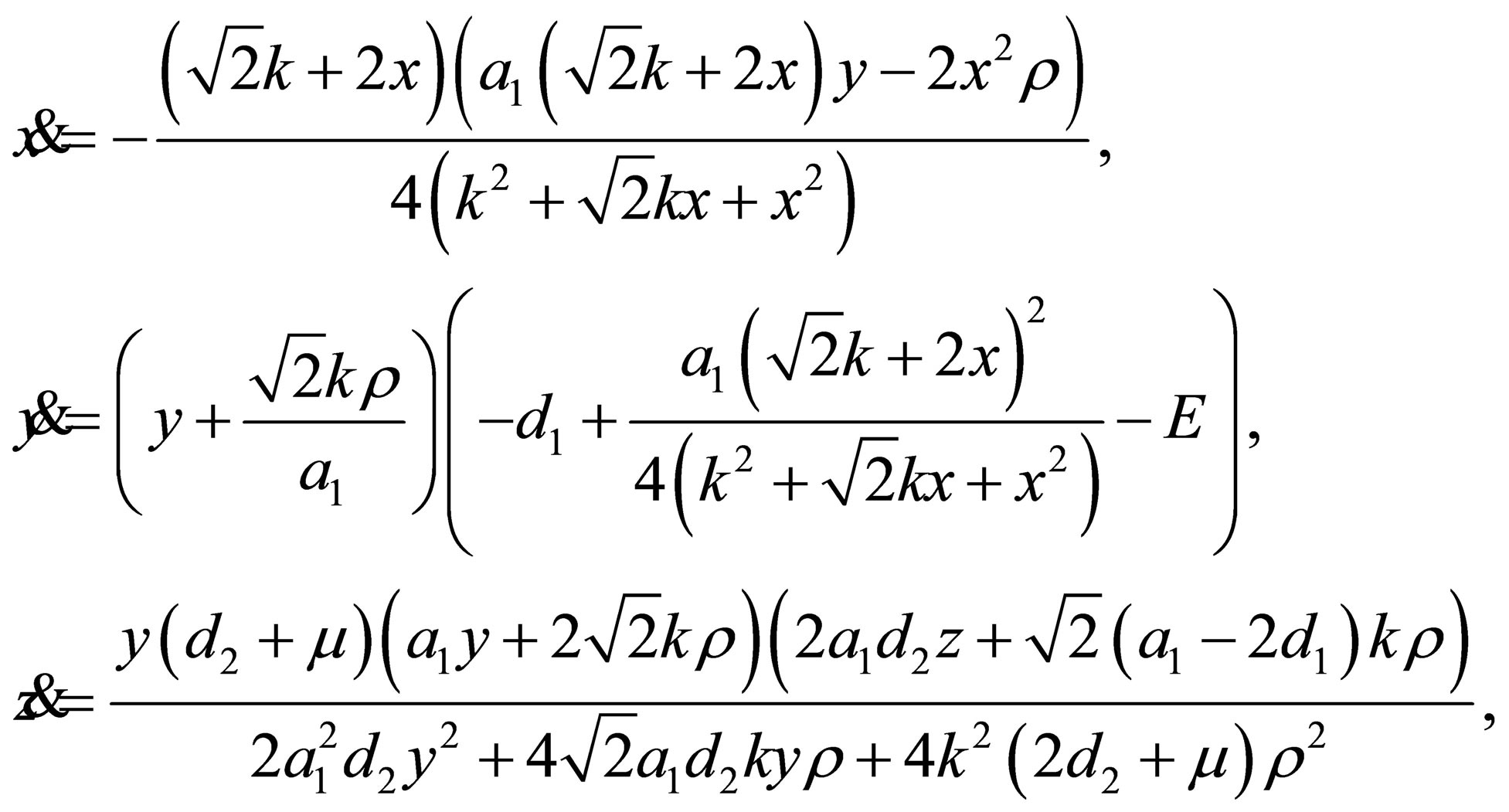(2)

where

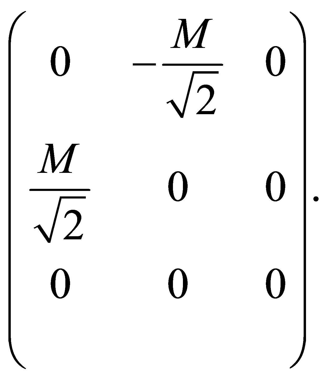
The matrix of the linear approximation of system (2) at the origin is

and the eigenvalues when are

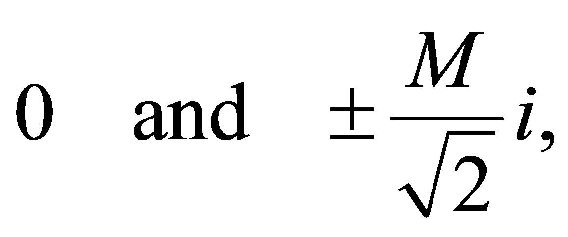
where. Then the origin of coordinates is a zero--Hopf equilibrium point of (2) when.

Now we apply a rescaling of the variables through the change of coordinates 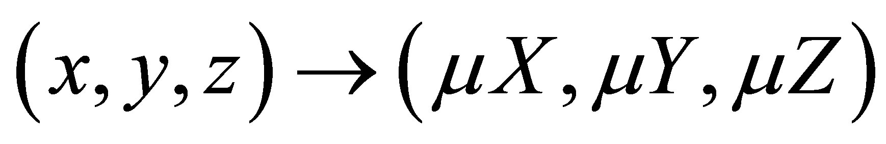obtaining the new differential system

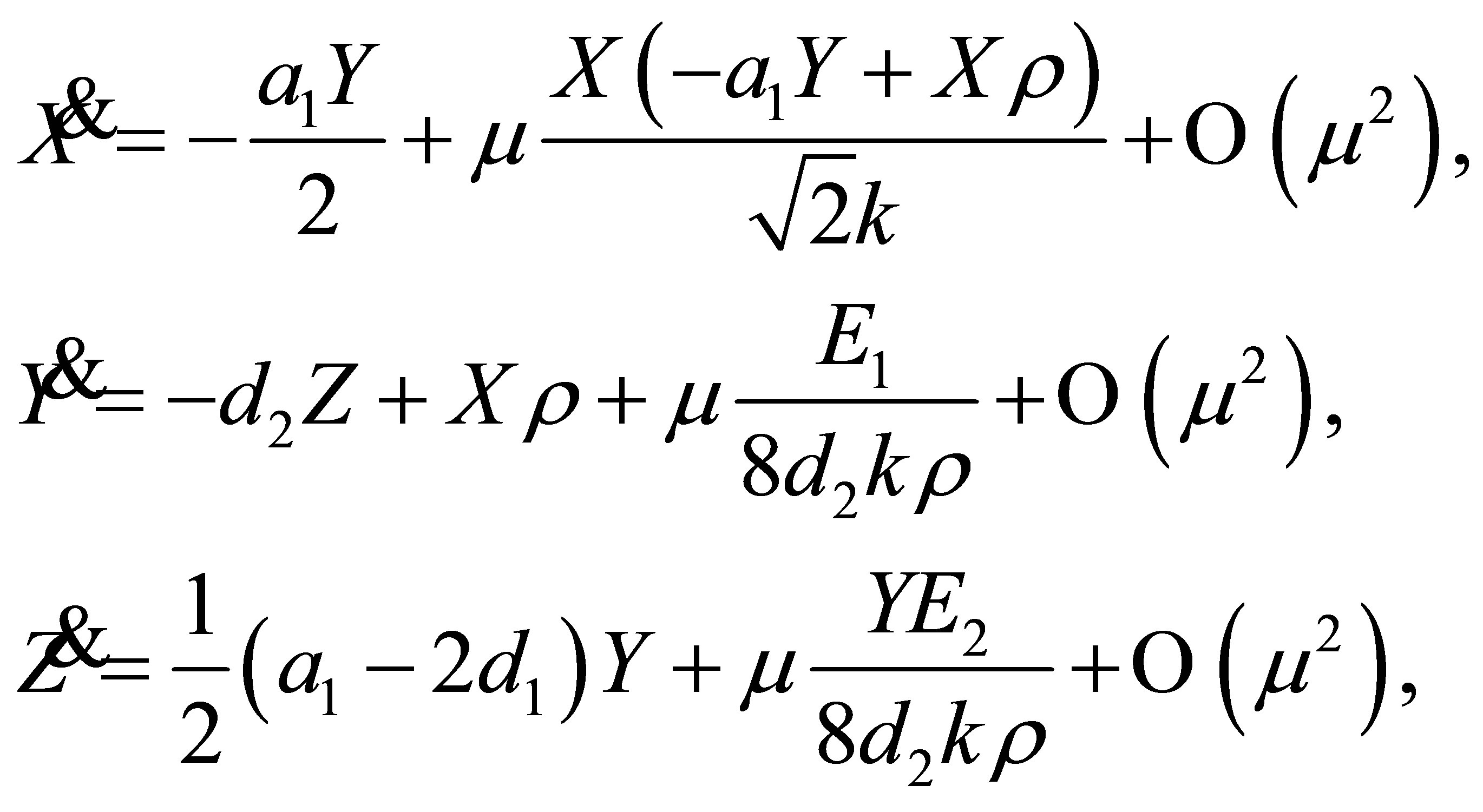(3)

where

Now we shall write the linear part at the origin of the differential system (2) when 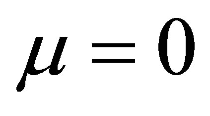into its real Jordan normal form, i.e. as

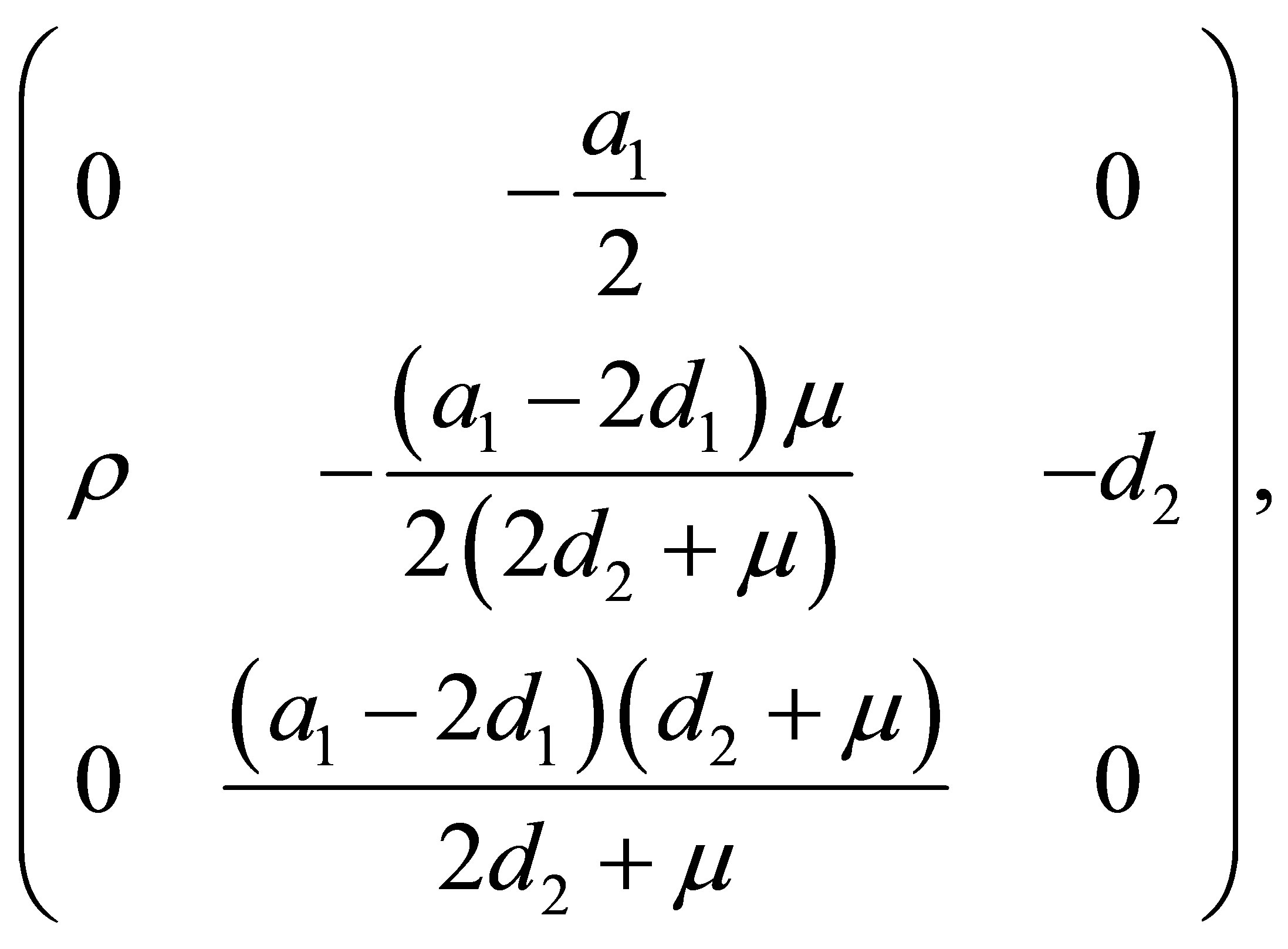
To do this, we apply a change of variables 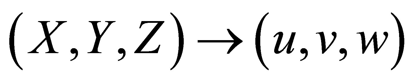, given by

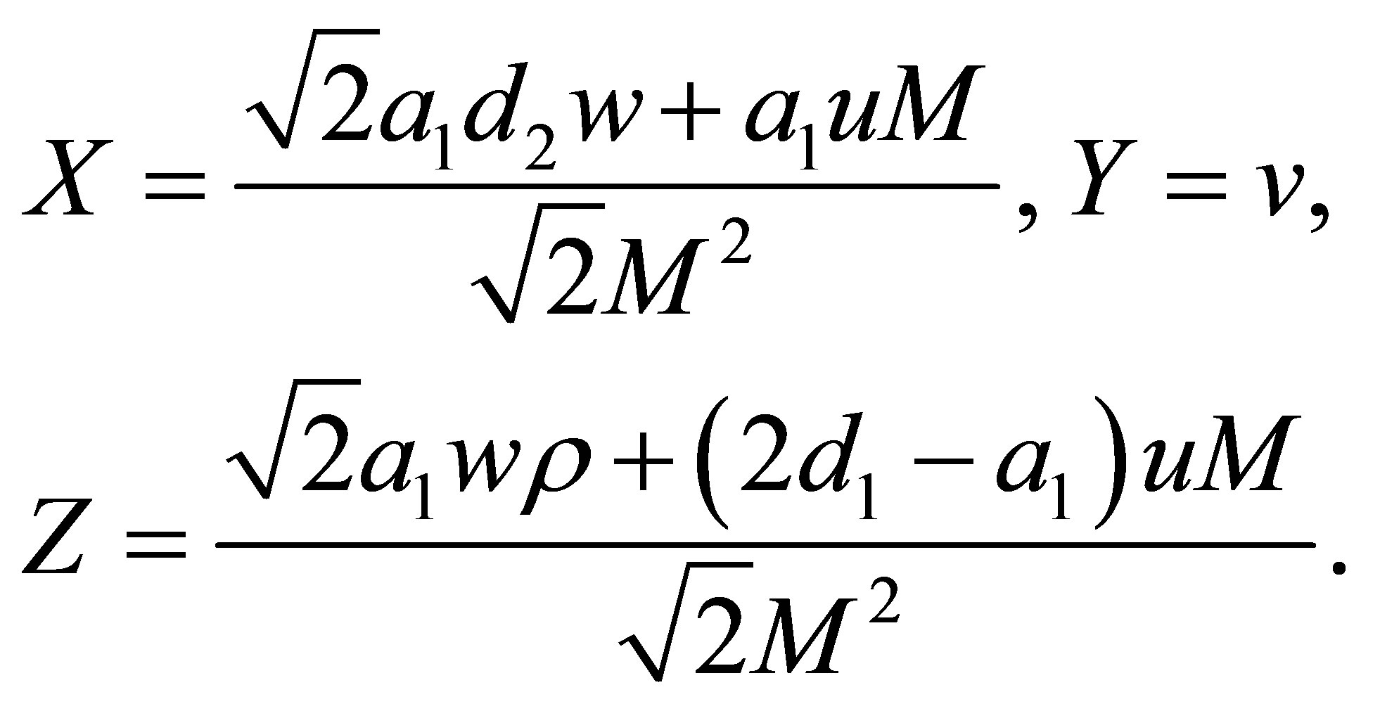(4)

In the new variables the differential system (3) writes

(5)

and this system has its linear part at the origin in the real Jordan normal form.

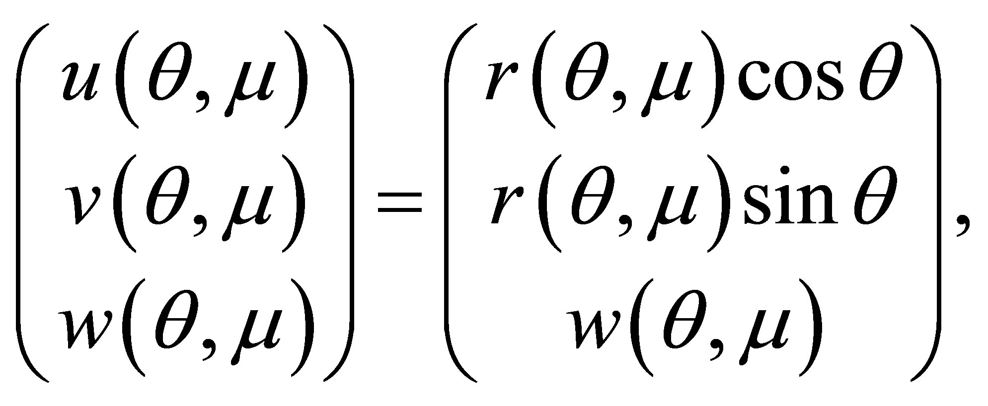
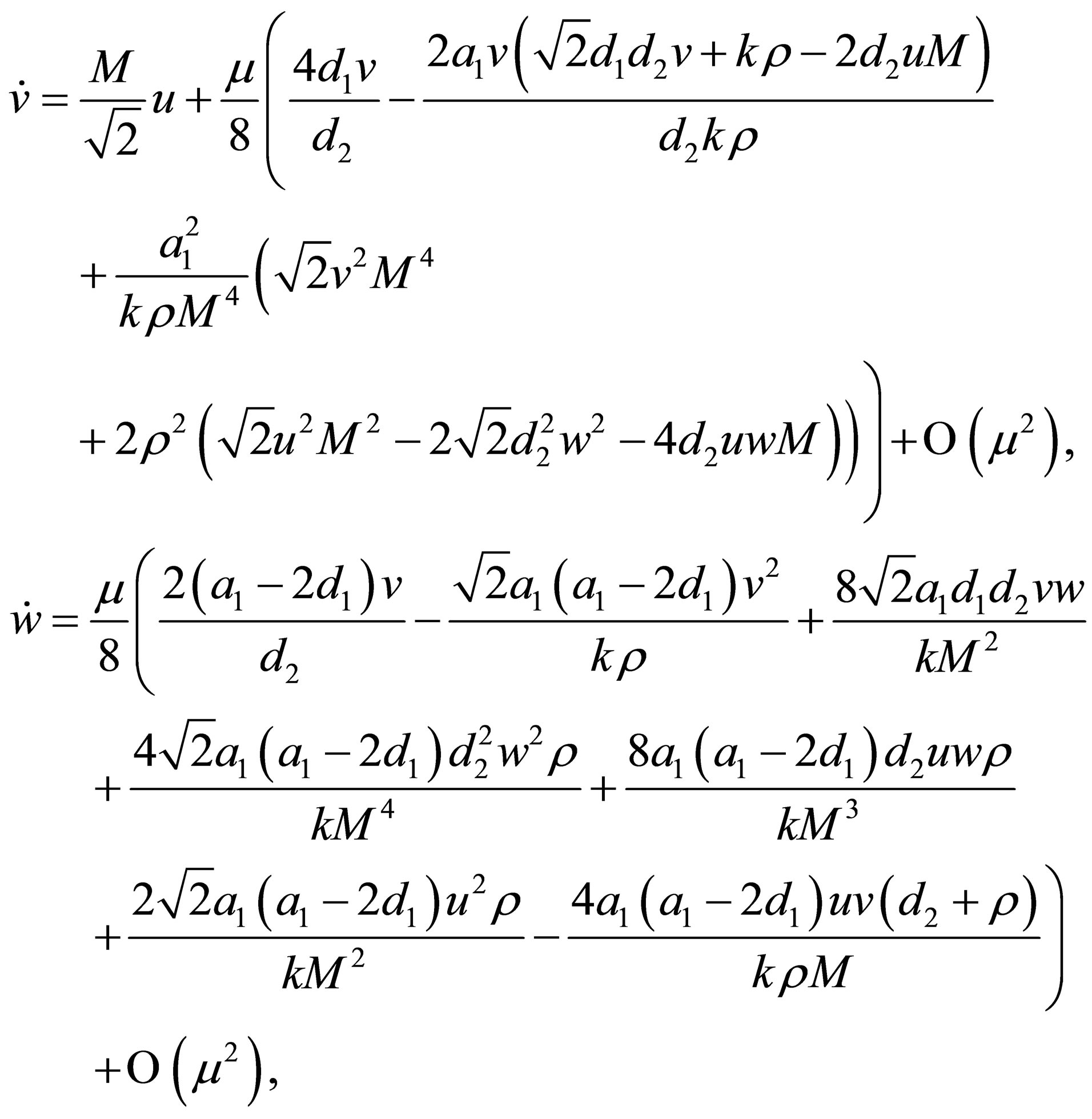
To apply the averaging theory we need to write the differential system (5) in cylindrical coordinates. Then we do the change of variables defined by, , and system (5) becomes

(6)

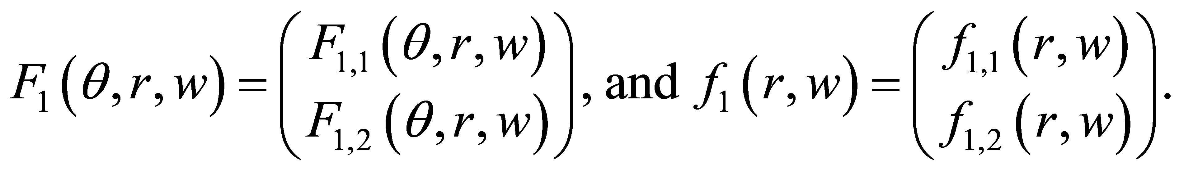
Using the notation of the appendix we have, , ,

It is immediate to check that system (6) satisfies all the assumptions of Theorem 3.

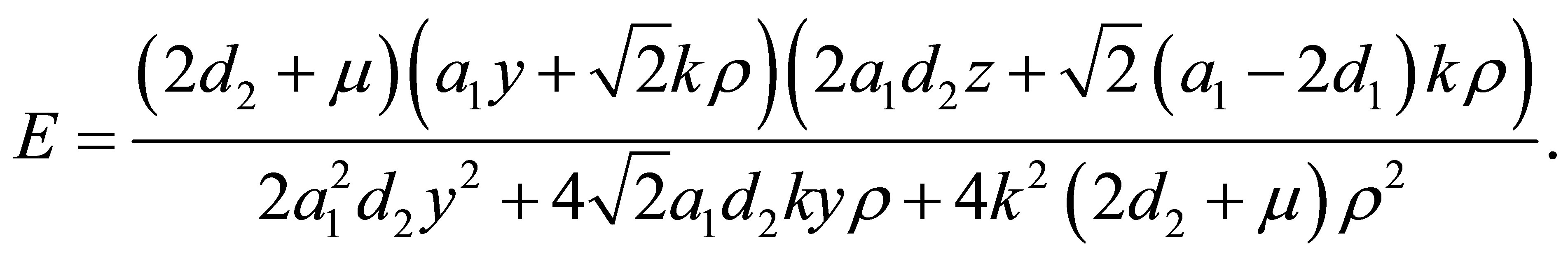
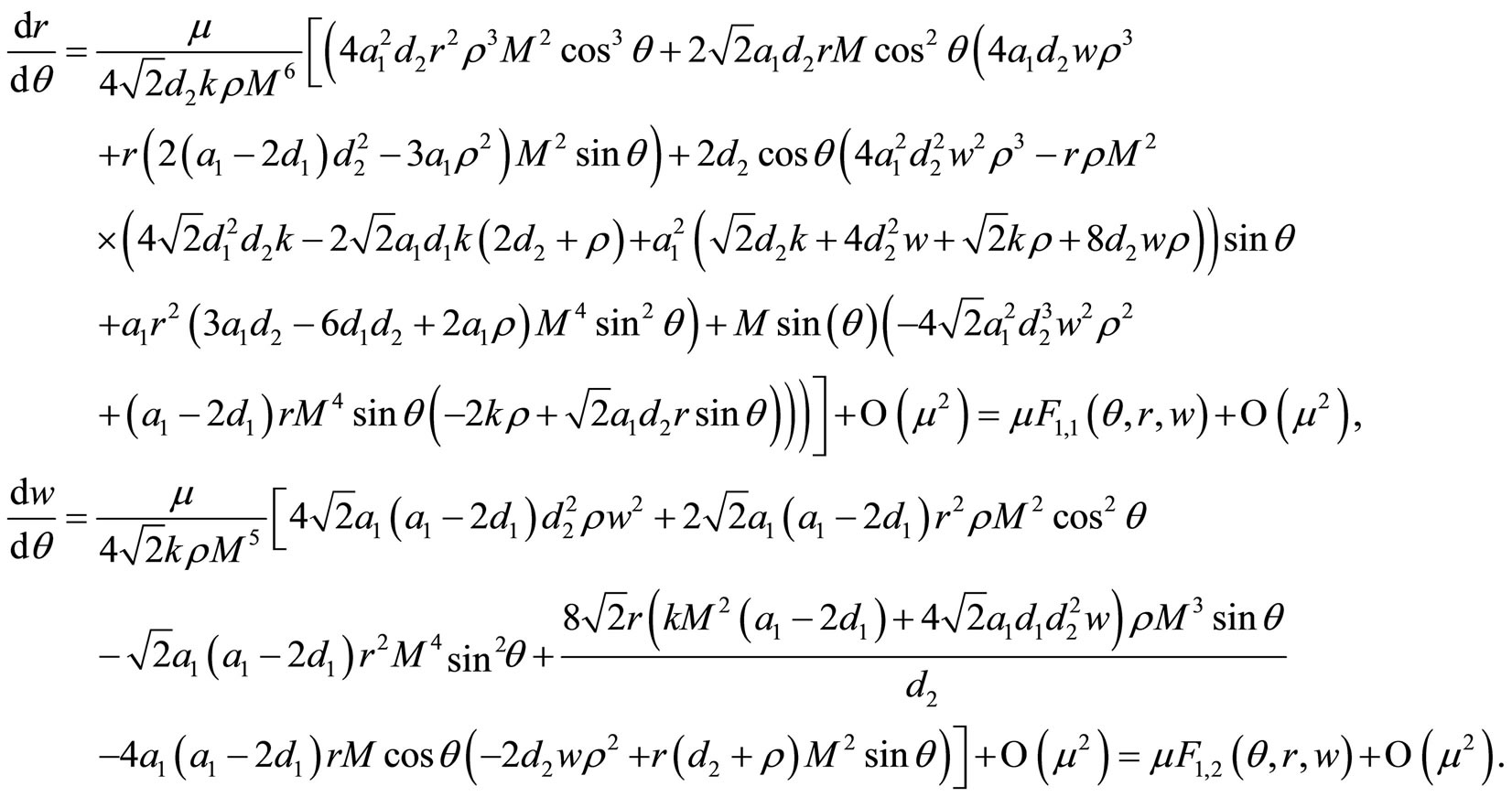
Now we compute the integrals (10), i.e.

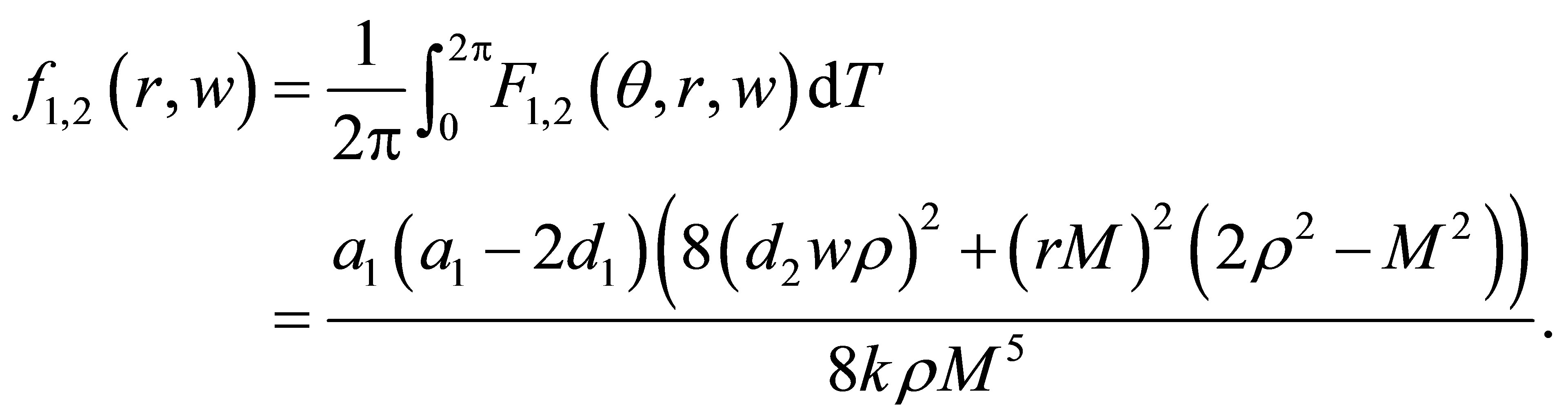
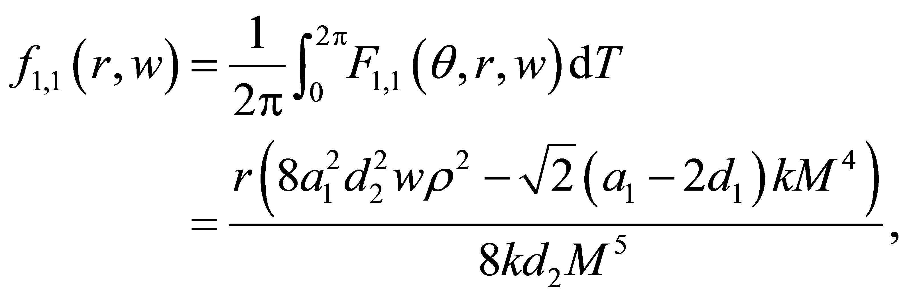
The system 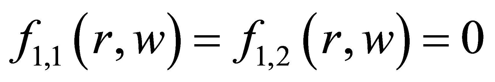has a unique solution, namely

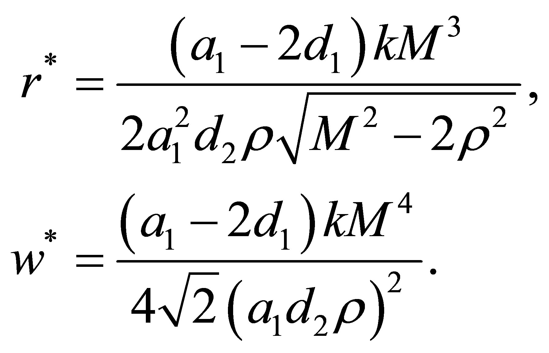
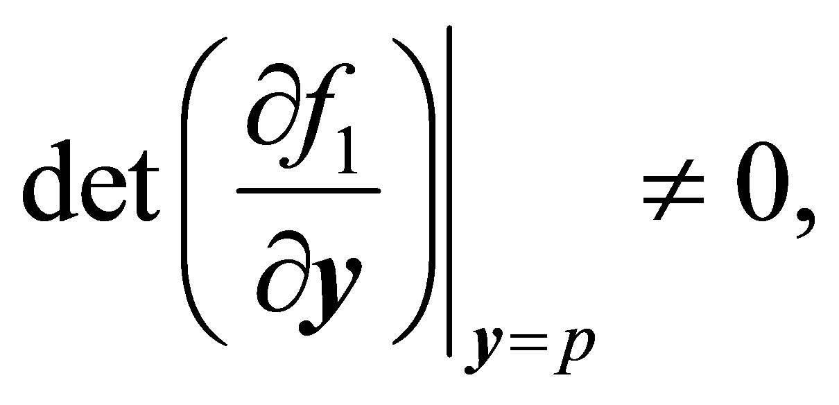
Finally, the Jacobian (11) at the point takes the value

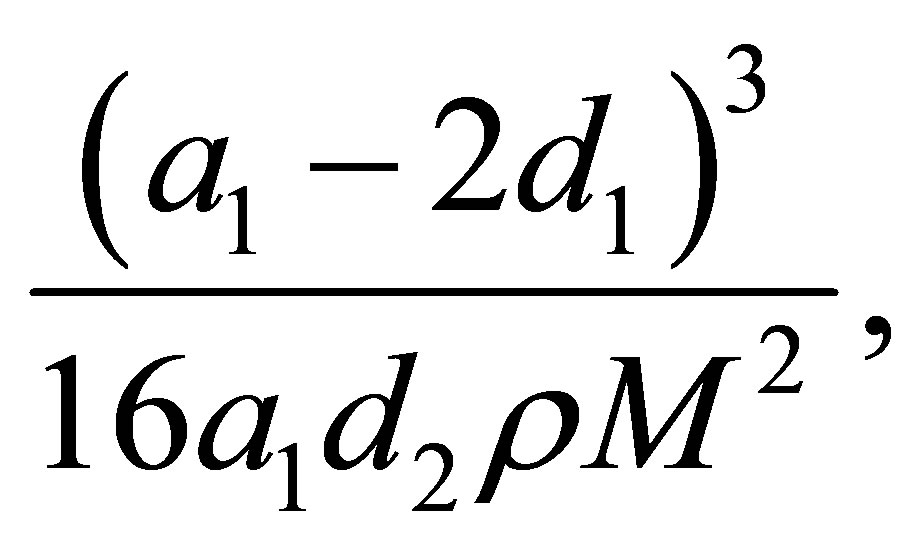
that by assumptions it is not zero. Then by the averaging theorem (Theorem 3) we have a periodic solution 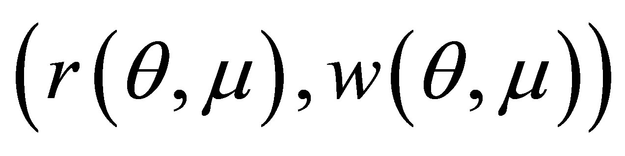of system (6) for sufficiently small such that 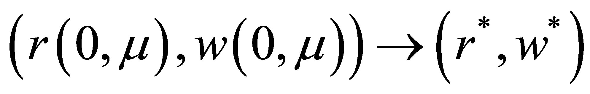when. Hence, the differential system (5) has the periodic solution

(7)

considering sufficiently small. Consequently, the differential system (3) has a periodic orbit

where

obtained from (7) through the change of variables (4). To finish, the differential system (2) has a periodic solution

for sufficiently small. Clearly, this periodic orbit tends to the origen of coordinates when. Therefore, it is a small amplitude periodic solution starting at the zero-Hopf equilibrium point located at the origin of coordinates when which correspond to the zeroHopf equilibrium point.

Following exactly the same computations we prove that at the equilibrium point also there exists a small amplitud periodic solution bifurcating from the equilibrium point. This concludes the proof of the theorem.

Appendix: The Averaging Theory of First Order

In this section we present some basic results related with the averaging theory that we will use in the proof of our main result.

The next theorem establish the existence and stability or instability of the periodic solutions for a periodic differential system. The proof of this theorem can be found in Theorems 11.5 and 11.6 of Verhulst [10].

Consider the differential systems

(8)

with, where is an open subset of, and is a small parameter. Moreover we assume that both and are T-periodic in. Now we also consider in the averaged differential equation

(9)

where

(10)

Under certain conditions the equilibrium solutions of the averaged Equation (9) correspond to T-periodic solutions of Equation (8).

Theorem 3Consider the two initial value problems (8) and (9) and suppose:

1), its Jacobian, its Hessian, and its Jacobian are defined, continuous and bounded by a constant independent of in and.

2) and are T-periodic in t (T independent of).

Then the following statements hold.

a) If p is an equilibrium point of the averaged Equation (9) and

(11)

then there exists a T-periodic solution of the differential Equation (8) such that 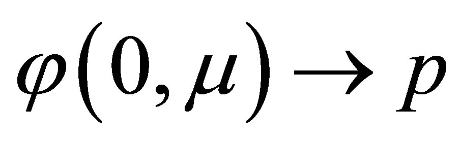as.

b) The stability or instability of the periodic solution 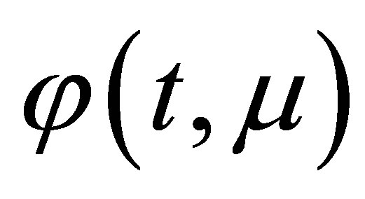is given by the stability or instability of the equilibrium point p of the averaged System (9). In fact the singular point p has the stability behavior of the Poincaré map associated to the limit cycle.

5. Conclusions

In this paper we study the coexistence of three species forming a tritrophic food chain model. Considering a linear grow for the lowest trophic species or prey, a type III Holling function responses for the middle and highest trophic species (first and second predator respectively). The explicit differential system modeling of this situation is system (1).

We prove that system (1) for adequate values of its parameters has two equilibria in the positive quadrant, and that each of these equilibria exhibits a small amplitud periodic solution bifurcating simultaneously of both equilibria. These two simultaneous Hopf bifurcations are degenerate in the sense that the real eigenvalue of the equilibria at the instant that the Hopf bifurcation takes place is zero, i.e., both equilibria are the called zero-Hopf equilibria. As far as we know, this is the first time that the phenomena appear in the literature related with food chain models.

6. Acknowledgements

The second author is partially supported by the grants MINECO/FEDER MTM 2008-03437, AGAUR 2009 SGR 410, ICREA Academia and FP7-PEOPLE-2012- IRSES-316338 and 318999.

REFERENCES

- J. Wang, J. Shi and J. E. Wei, “Predator-Prey System with Strong Allee Effect in Prey,” Journal of Mathematical Biology, Vol. 62, No. 3, 2011, pp. 291-331. http://dx.doi.org/10.1007/s00285-010-0332-1
- S. M. Baer, B. Li and H. L. Smith, “Multiple Limit Cycles in the Standard Model of Three Species Competition for Three Essential Resources,” Journal of Mathematical Biology, Vol. 52, No. 6, 2006, pp. 745-760. http://dx.doi.org/10.1007/s00285-005-0367-x
- X. Li, H. Wang and Y. Kuang, “Global Analysis of a Stoichiometric Producer-Grazer Model with Holling Type Functional Responses,” Journal of Mathematical Biology, Vol. 63, No. 5, 2011, pp. 901-932. http://dx.doi.org/10.1007/s00285-010-0392-2
- H. Freedman and P. Waltman, “Mathematical Analysis of Some Three-Species Food-Chain Models,” Mathematical Biosciences, Vol. 33, No. 3-4, 1977, pp. 257-276. http://dx.doi.org/10.1016/0025-5564(77)90142-0
- H. I. Freedman and J. W. H. So, “Global Stability and Persistence of Simple Food Chains,” Mathematical Biosciences, Vol. 76, No. 1, 1985, pp. 69-86. http://dx.doi.org/10.1016/0025-5564(85)90047-1
- T. C. Gard, “Persistence in Food Chains with General Interactions,” Mathematical Biosciences, Vol. 51, No. 1-2, 1980, pp. 165-174. http://dx.doi.org/10.1016/0025-5564(80)90096-6
- J. P. Francoise and J. Llibre, “Analytical Study of a Higher-Order Hopf Bifurcation in a Tritrophic Food Chain Model,” Applied Mathematics and Computation, Vol. 217, No. 17, 2011, pp. 7146-7154. http://dx.doi.org/10.1016/j.amc.2011.01.109
- A. Buică and J. Llibre, “Averaging Methods for Finding Periodic Orbits via Brouwer Degree,” Bulletin des Sciences Mathématiques, Vol. 128, No. , 2004, pp. 7-22. http://dx.doi.org/10.1016/j.bulsci.2003.09.002
- J. Sanders, F. Verhulst and J. Murdock, “Averaging Method in Nonlinear Dynamical Systems,” 2nd Edition, Applied Mathematical Sciences, Vol. 59, Springer, New York, 2007.
- F. Verhulst, “Nonlinear Differential Equations and Dynamical Systems,” 2nd Edition, Universitext, Springer-Verlag, Berlin, 1996.
- K. Cheng, “Uniqueness of a Limit Cycle of a PredatorPrey System,” SIAM Journal on Mathematical Analysis, Vol. 12, No. 4, 1981, pp. 541-548. http://dx.doi.org/10.1137/0512047
- B. Deng, “Food Chain Chaos with Canard Explosion,” Chaos, Vol. 14, No. 4, 2004, pp. 1083-1092. http://dx.doi.org/10.1063/1.1814191
- B. Deng and G. Hines, “Food Chain Chaos Due to Shilnikov’s Orbit,” Chaos, Vol. 12, No. 3, 2002, pp. 533-538.
- Yu. A. Kuznetsov, O. De Feo and D. Rinaldi, “Belyakov Homoclinic Bifurcations in a Tritrophic Food Chain Model,” SIAM Journal on Mathematical Analysis, Vol. 62, 2001, pp. 462-487. http://dx.doi.org/10.1137/S0036139900378542
- R. May, “Limit Cycles in Predator-Prey Communities,” Science, Vol. 177, No. 4052, 1972, pp. 900-902. http://dx.doi.org/10.1126/science.177.4052.900
- S. Muratori and S. Rinaldi, “A Dynamical System with Hopf Bifurcations and Catastrophes,” Applied Mathematics and Computation, Vol. 29, 1989, pp. 1-15. http://dx.doi.org/10.1016/0096-3003(89)90036-2
- C. S. Holling, “Some Characteristics of Simple Types of Predation and Parasitism,” Entomological Society of Canada, Vol. 91, 1959, pp. 385-398. http://dx.doi.org/10.4039/Ent91385-7
- J. Guckenheimer, “On a Codimension Two Bifurcation, Dynamical Systems and Turbulence, Warwick 1980 (Coventry, 1979/1980),” Lecture Notes in Mathematics, Vol. 898, No. 654886, Springer, Berlin, 1981, pp. 99-142.
- J. Guckenheimer and P. Holmes, “Nonlinear Oscillations, Dynamical Systems, and Bifurcations of Vector Fields,” Applied Mathematical Sciences, Vol. 42, Springer Verlag, 2002.
- M. Han, “Existence of Periodic Orbits and Invariant Tori in Codimension Two Bifurcations of Three-Dimensional Systems,” Journal of Systems Science and Mathematical Sciences, Vol. 18, No. 4, 1998, pp. 403-409.
- Yu. A. Kuznetsov, “Elements of Applied Bifurcation Theory,” 3rd Edition, Applied Mathematical Sciences, Vol. 12, Springer-Verlag, New York, 2004.
- J. Scheurle and J. Marsden, “Bifurcation to Quasi-Periodic Tori in the Interaction of Steady State and Hopf Bifurcations,” SIAM Journal on Mathematical Analysis, Vol. 15, No. 6, 1984, pp. 1055-1074. http://dx.doi.org/10.1137/0515082
- I. Baldomá and T. M. Seara, “Brakdown of Heteroclinic Orbits for Some Analytic Unfoldings of the Hopf-Zero Singulairty,” Journal of Nonlinear Science, Vol. 16, No. 6, 2006, pp. 543-582. http://dx.doi.org/10.1007/s00332-005-0736-z
- I. Baldomá and T. M. Seara, “The Inner Equation for Genereic Analytic Unfoldings of the Hopf-Zero Singularity,” Discrete and Continuous Dynamical Systems: Series B, Vol. 10, No. 2-3, 2008, pp. 232-347.
- H. W. Broer and G. Vegter, “Subordinate Silnikov Bifurcations Near Some Singularities of Vector Fields Having Low Codimension,” Ergodic Theory and Dynamical Systems, Vol. 4, No. 4, 1984, pp. 509-525. http://dx.doi.org/10.1017/S0143385700002613
- A. R. Champneys and V. Kirk, “The Entwined Wiggling of Homoclinic Curves Emerging from Saddle-Node/Hopf Instabilities,” Physics D: Nonlinear Phenomena, Vol. 195, No. 1-2, 2004, pp. 77-105. http://dx.doi.org/10.1016/j.physd.2004.03.004