Open Journal of Modern Hydrology
Vol.3 No.1(2013), Article ID:27235,10 pages DOI:10.4236/ojmh.2013.31005
Evaluation of a Simple Hydraulic Resistance Model Using Flow Measurements Collected in Vegetated Waterways

1Department of Water Engineering & Management, Faculty of Engineering Technology, University of Twente, Enschede, The Netherlands; 2HKV Consultants, Lelystad, The Netherlands; 3Department of Earth System Analysis, Faculty of Geosciences, Utrecht University, Utrecht, The Netherlands.
Email: huthoff@hkv.nl, m.w.straatsma@uu.nl, d.c.m.augustijn@utwente.nl, s.j.m.h.hulscher@utwente.nl
Received October 11th, 2012; revised November 15th, 2012; accepted November 28th, 2012
Keywords: Hydraulic Roughness; Vegetation; River Flow; Floodplains; ADCP Measurements
ABSTRACT
A simple idealized model to describe the hydraulic resistance caused by vegetation is compared to results from flow experiments conducted in natural waterways. Two field case studies are considered: fixed-point flow measurements in a Green River (case 1) and vessel-borne flow measurements along a cross-section with floodplains in the river Rhine (case 2). Analysis of the two cases shows that the simple flow model is consistent with measured flow velocities and the present vegetation characteristics, and may be used to predict a realistic Manning resistance coefficient. From flow measurements in the river floodplain (case 2) an estimate was made of the equivalent height of the drag dominated vegetation layer, as based on measured flow characteristics. The resulting height corresponds well with the observed height of vegetation in the floodplain. The expected depth-dependency of the associated Manning resistance coefficient for could not be detected due to lack of data for relatively shallow flows. Furthermore, it was shown that topographical variations in the floodplain may have an important impact on the flow field, which should not be mistaken as roughness effects.
1. Introduction
Various studies have shown that if vegetation penetrates a significant part of the water column then a constant Manning resistance value is no longer adequate to describe the hydraulic resistance for varying flow conditions [1-5]. These studies have shown that the hydraulic resistance due to vegetation (in terms of Manning’s n) tends to decrease with increasing water level. No methodology to describe such behavior is generally accepted despite intense research efforts in recent years. This is partly due to the empirical nature of proposed relationships and the difficulties in deriving generally applicable methods due to the complexity of flow around vegetation. In particular, hydraulic resistance parameters determined in the field are unavoidably contaminated with additional external influences, such as geometrical variations of the channel, density currents, sediment interactions or surface waves [6]. Furthermore, collecting flow data in natural vegetated waterways is in itself a tricky task: the presence of vegetation obstructs detailed flow velocity sampling [7]. In particular when vegetation is abundant and has a large impact on the flow field, accurate data sampling is difficult. As a result, studies where flow characteristics are measured in vegetated waterways are relatively scarce [8], they are case-specific and, due to the complexity of the environment, are difficult to interpret (see [9], where flume studies are used as a reference to field measurements).
Most experimental studies on hydraulic resistance of vegetation are conducted in laboratory flumes, where it is possible to minimize hydraulic impacts due to other external influences [10-13]. That way, investigations of vegetative hydraulic resistance allow isolation of the impact of specific vegetation characteristics (such as stem width, height, flexibility). These studies have revealed that flow through vegetation is difficult to describe based on geometrical conditions of the vegetation alone, even if vegetation is described in a simplified way as cylindrical stems. A recurring complication of these hydraulic resistance models is the need for a general representation of energy losses associated with turbulent mixing patterns. Such energy-loss representations may enter the flow models in the form of a turbulent mixing length [14-17]. Flow descriptions that include the mixing length concept only have practical value if the mixing length is directly related to measurable quantities. Such relations have been proposed [16,18,19], but due to lack of theoretical justification their general applicability remains questionable. Other, more general, approaches include k-ε turbulence models, which explicitly describe the transport of turbulent energy [20-22]. However, these methods require considerably larger computational effort, in particular if applied in models on river-reach scales.
Alternatively, a simple vegetation resistance model has been proposed by Huthoff et al. [23] that includes only measurable quantities. The model requires knowledge of a vegetation drag coefficient CD, the average vegetation height k, stem diameter D and a representative spacing between neighboring plants s (see also [24]). Among these parameters, only the drag coefficient cannot be directly obtained from vegetation dimensions, but is to be determined from flow experiments. It appears that the CD-value is species-specific [25] and is a function of the Reynolds number [26], stem aspect ratio [27], vegetation distribution density [28,29] and foliage and streamlining effects [30,31].
In the current work we investigate whether the simplified model proposed in [23] is consistent with flow measurements in the field, and whether it provides a potential candidate for integration with river-reach flow models. Two case-studies with flow in vegetated waterways are considered (Figure 1). First, measured flow velocities and vegetation characteristics in a Green River are evaluated against predictions of the hydraulic resistance model (case 1). It is shown that the model provides an acceptably accurate estimate of the average flow velocity, as based on general vegetation characteristics. Next, flow velocities are measured in a natural floodplain at different discharge magnitudes (case 2). In this case study, no detailed information about the vegetation characteristics was available. Therefore, we evaluate whether the measured dynamic behavior of the hydraulic resistance is consistent with the vegetation resistance model. It is shown that the proposed model describes the vegetation resistance well, but that because of the weak dynamic behavior of the hydraulic resistance, and the lack of data at shallow flows, also a simple wall-roughness model may be used for the considered flow conditions.
2. Case 1: Fixed-Point Measurements
2.1. Study Location
In February 2005, during a high-discharge event in the Rhine river a Green River1 was deployed to convey surplus river discharge. Due to its relative homogeneous geometrical boundaries, the Green River is suitable for measurements of the hydraulic effect of the present vegetation. The aerial picture in Figure 2 shows the study area, including the bridge from where measurements were performed. The flow direction in this picture is from east (right) to west (left). Figure 3 shows the presence of vegetation on the channel bed of the Green River, as observed during dry conditions. Note that the Green River includes a central sub-channel (indicated in Figure 2 and also just visible in right panel of Figure 3). The sub-channel is always wet but is closed at both ends, and therefore does not convey water.
2.2. Methodology and Results
The bridge that spans the Green River was used to tether a float from, to record the flow velocities below. Figure 4 shows a picture of the bridge on the 17th of February 2005, the day that data were collected. Three locations
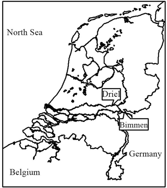
Figure 1. A map of the Netherlands indicating locations of the two case studies (Driel and Bimmen).
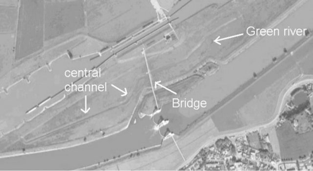
Figure 2. Aerial picture of the Green river at Driel. Also, the central (sub-) channel is indicated.
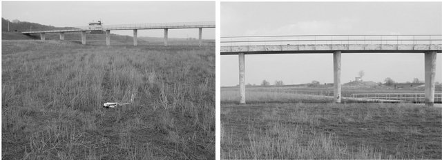
Figure 3. The measurement location at Driel during dry conditions (pictures: M.W. Straatsma).
along the bridge were used for measurements: one in the central sub-channel of the Green River (Location 2) and two locations well-separated to either side of the central sub-channel (Locations 1 and 3). These latter two locations have similar bed coverage characteristics (as seen in Figure 3) and are thus expected to be hydraulically equivalent.
An RD Instruments Acoustic Doppler Current Profiler (ADCP) was used to record flow velocity profiles. The ADCP resolves the three-dimensional flow vector at various user-defined depths. Due to the size of the ADCP itself, and the inability of the ADCP to measure flow velocities immediately below the device, flow velocities were measured downwards from 46 cm below the water surface, at depths 10 cm apart. An average ensemble interval of 6 s was used to determine the mean streamwise velocity. Near the bed, large fluctuations in flow velocities were measured (Figure 5). The fluctuations are likely due to the presence of vegetation. Vegetation parameters were independently measured after the flood, giving an average height of k = 37.5 cm, an average stem width of the vegetation of D = 3.7 mm, an average surface density of m = 51 stems/m2, leading to an average spacing between plants of s = 13.6 cm.
Figure 5 shows the measured flow velocity profiles for the three locations along the bridge. The graphs also show the profiles of the average streamwise velocities, together with 16- and 84-percentile error boundaries. These boundaries correspond to a 1σ standard deviation if errors were distributed normally. The flow depth h is measured independently by the ADCP, as stated above the graphs in Figure 5. Also stated are the depth-averaged flow velocities in the surface layer Us. representing flow above the vegetation.
The graphs in Figure 5 show that, between the three measurement locations, the depth-averaged flow velocity in the deepest location (Location 2) is slightly smaller than for the other two locations. This may seem an unexpected result, because for equal bed resistance one would expect larger flow velocities at larger depths.
However, it appears that at Location 2 not the entire water column contributes to discharge capacity. As mentioned before, the sub-channel at Location 2 is closed at both ends, thus partially obstructing flow. Another effect that may cause the flow in the central channel to slow down is the presence of a small bridge (see Figure 3). This small bridge was entirely flooded during the highdischarge event in February 2005 (see Figure 4), thus obstructing flow near the central sub-channel. Consequently, we consider the flow measurements at Location 1 and Location 3 in Figure 5 more representative of the hydraulic response due to bed vegetation. In the remainder, the measurements from Location 2 in the central sub-channel are therefore discarded for the analysis of hydraulic resistance due to vegetation.
Finally, the energy slope i was determined by tracking a float from a fixed location on the river bank (for float tracking methodology, see [32]). This resulted in an average value for the energy slope of i = 9.2 × 10⁻⁵, having an error of about 20%.
2.3. Comparison to Model Predictions
Here we consider the simple model for the hydraulic resistance of vegetation as proposed by Huthoff et al. [23] (also see [24]). In this model, the flow velocity in the vegetation layer (or resistance layer) Ur is described
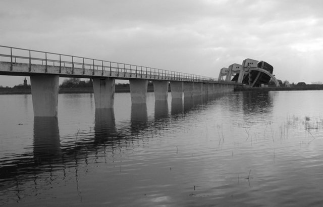
Figure 4. The measurement location at Driel during high discharge on February 17, 2005 (picture: M.W. Straatsma).
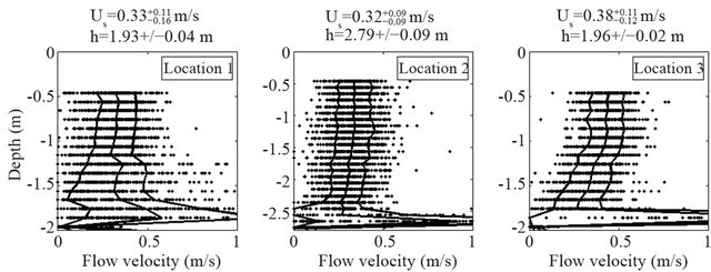
Figure 5. Velocity measurements at three different locations for case 1. The average velocity profile and 16- and 84-percentile boundaries are shown in each of the graphs. Stated above each graph, Us is the depth-averaged velocity in the surface layer and h the flow depth.
separately from flow in the surface layer Us. Together, they give an estimate of the average flow velocity over the total depth UT:
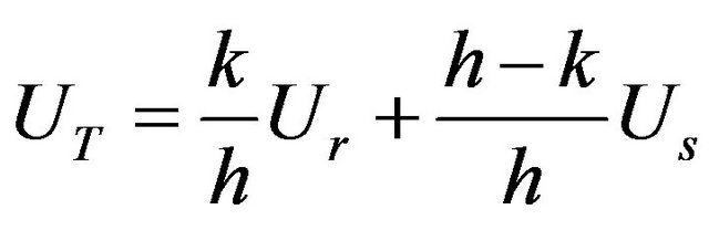 (1)
(1)
The depth-averaged flow velocity in the surface layer is represented by the power law
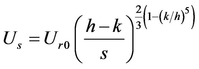 (2)
(2)
where the power exponent reduces to a constant value of 2/3 if the total flow depth h is at least twice as large as vegetation height k. The representative separation between homogeneously distributed cylindrical vegetation elements vegetation (s), is calculated as [23]:
 (3)
(3)
The average flow velocity in between the vegetation (in the vegetation layer) is estimated as
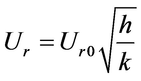 (4)
(4)
In Equations (2) and (4) the characteristic scaling velocity Ur0 is given by
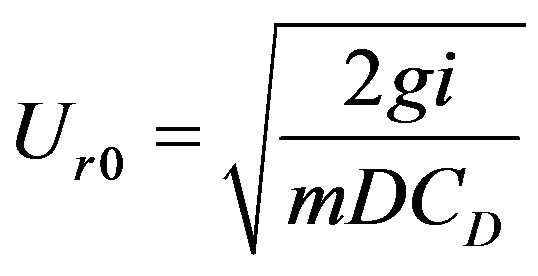 (5)
(5)
with g the gravitational acceleration, i the (energy) slope, m the number of vegetation elements per unit bed area, D the stem diameter and CD the dimensionless drag coefficient. Using the earlier stated vegetation parameters in Section 2.2 the average flow velocities can be predicted using Equations (1)-(5). The only unknown parameter is the drag coefficient for which we adopt CD = 1.8 [33].
Figure 6 shows the predicted flow velocities for the resistance layer, the surface layer, the entire flow depth and Manning’s n based on a 20% standard deviation in the measured vegetation parameters and a 10% standard deviation in adopted CD-value. Comparing the measured values for the surface velocity in Figure 5 (Us ≈ 0.33 - 0.38 m/s) with the predicted value in Figure 6 (Us ≈ 0.38 m/s), shows that the applied vegetation resistance model gives quite good results.
2.4. Discussion
For the considered case in the Green River we were only able to measure flow velocities in the surface layer, because the presence of vegetation distorted measurement near the bed (see Figure 5). Therefore, we cannot evaluate the predicted depth-averaged flow velocities of the vegetation layer Ur and of the total flow depth UT (as given in Figure 6) against field measurements. However, using the predicted values for UT, a Manning resistance parameter n can be calculated, which subsequently allows comparison with values cited in literature for grasslined channels. Manning’s equation is given as:
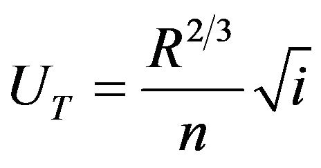 (6)
(6)
which has the property that the resistance coefficient n is practically constant for hydraulically rough turbulent flow over a fixed bed [34]. Inserting the measured flow depth (at Location 3, see Figure 5) and the predicted values for UT yields Manning resistance coefficients n = 0.045 +/− 0.007 m−1/3s. This calculated n-value is consistent with the Manning values cited in literature for grass-lined floodplains. For “high grass” Chow [35] states a general value of n = 0.035, with a lower boundary of n=0.030 and an upper boundary of n = 0.050 m−1/3s. However, as was mentioned in the introduction, n generally does not remain constant for flows over vegetation.
Figure 7 shows how the model Equations (1)-(5) together with Manning’s law, Equation (6), lead to a depthdependent Manning coefficient. It can be seen that at flow depths that are greater than the one considered, the n-value is expected to decrease. However, the projected changes for large flow depths appear to be quite insignificant, and also a constant Manning’s n may be used. Shallower flows are expected to yield considerably stronger changes in n, with nearly doubled values for just submerged vegetation. Similar trends have been reported in empirical studies of vegetation resistance [1-5]. In particular, the study of Wilson and Horritt [4] shows that the Manning coefficient becomes practically constant if the flow depth is much larger than the vegetation height.
We conclude that the model by Huthoff et al. [23] can be used to give a reliable estimate of the effective roughness under field conditions and that, qualitatively, predicted trends of the roughness model agree with trends cited in the literature.
3. Case 2: Vessel-Borne Flow Measurements
3.1. Study Location
In 1998 a high-discharge event occurred on the Rhine River with a maximum recorded discharge of 9413 m3/s
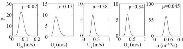
Figure 6. Probability densities of predicted flow velocities (μ = mean value) based on uncertainty in the drag coefficient and variations in measured vegetation characteristics.
(recorded on November 4th at station Lobith). During the high-discharge event, vessel-borne ADCP measurements were carried out along a cross-section of the River [36]. See Figure 8 for the research vessel and the ADCP device, and Figures 9 and 10 for the sampled river crosssection. Water flows from the east to the west, which in Figure 9(b) is from the lower right to the upper left. The flood-plain on the southern bank is clearly visible in Figure 9, as is the embankment that separates it from the main channel. Groynes are present on the northern bank and also further upstream on the southern bank. The flood-plain is covered with grassland.
3.2. Methodology and Results
Flow data were collected along a cross-section at km 863.9 in the Rhine on four consecutive days from November 3 to 6 and then again from November 9 to 11. The discharge peak occurred at November 4 and decreased quite rapidly thereafter. On November 9 the wa-
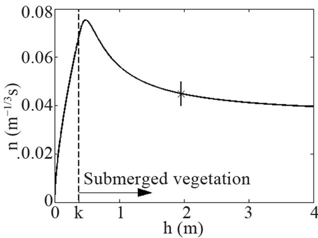
Figure 7. Manning’s resistance coefficient n as predicted by the model Equations (1)-(5). The “x” symbol corresponds to the average conditions at Location 3 in the Green River.
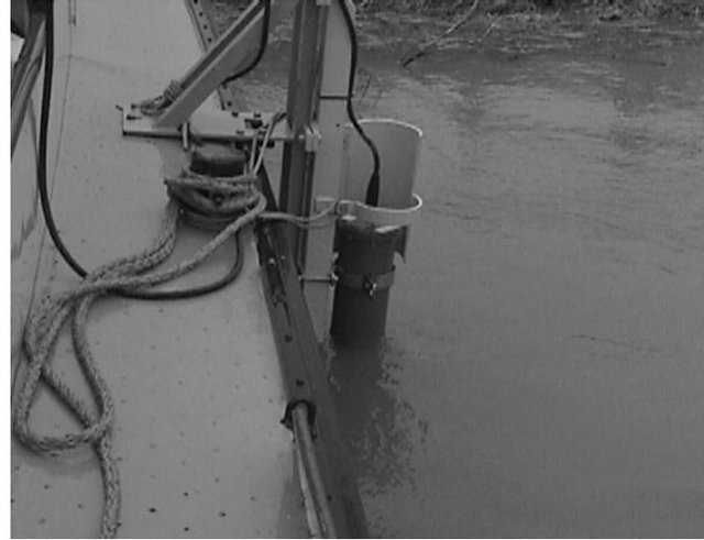
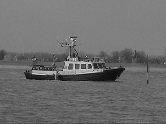
Figure 8. The used research vessel for flow measurements in the Rhine River in November 1998 (left). The picture on the right shows the attached ADCP (pictures: aqua vision).
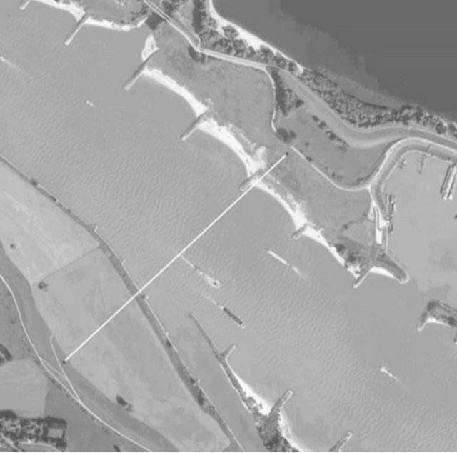
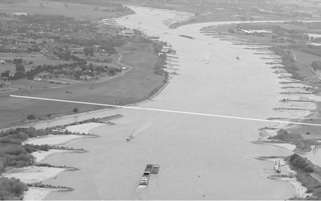
Figure 9. Aerial pictures of the study area. The white line shows the measurement transect.
ter level had dropped to a level that flow measurements were no longer possible in the floodplain. On each day, flow measurements were collected for multiple transits along the river cross-section (Figure 10). The transits outline a narrow cross-sectional strip of the channel, for which the best fit straight-line was defined as the equivalent transect (dotted line in Figure 10). In the subsequent analysis, all measurements are mapped onto the equivalent transect.
In Figure 11 an example is shown of one of the sampling runs. Flow velocities were measured below the research vessel at depths 25 cm apart with the highest measuring point 1.32 m below the water surface. Lateral sampling separations were on average 4 m, depending on the travelling speed of the vessel. A region of about 60 cm above the channel bed could not be reliably sampled for flow velocities, partly due to presence of obstructing objects (vegetation) or debris. The measurements were performed in bottom-track mode, correcting measurements for vessel movement and thus giving flow velocities with respect to the detected fixed bed. However, a bottom layer of sediment may be dragged along with the flow, which the ADCP interprets as a fixed bed and subsequently gives a bias towards underestimation of flow velocities. The measurements used here are corrected for this effect by comparison with independent GPS data of the research vessel. Details of this procedure are described in [36].
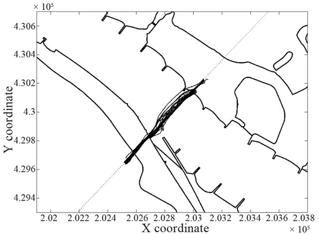
Figure 10. The measurement trajectories near rkm 863.9. The dotted line depicts the equivalent transect.
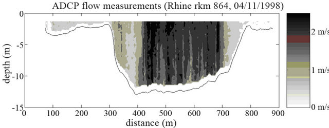
Figure 11 shows that lower flow velocities are recorded in the shallower regions of the cross-section. However, a striking feature in the measurement results is that near the deepest part of the channel there appears to be a local minimum in flow velocities (near the lateral coordinate of 380 m). This feature is also observed in the remaining measurement runs (not shown here). The overview of the study area in Figure 9 may provide an explanation for this observation. Just upstream of the channel cross-section a small channel merges with the Rhine on its southern bank. The local dip in flow velocities is likely due to enhanced mixing in the wake of the confluence zone.
To be able to compare the measured flow velocities in the floodplains to model predictions of vegetation resistance, we depth-averaged the measured flow velocities. Next, we grouped all data collected on the same day, assuming that within this time frame no significant hydraulic changes occurred in the system. Figure 12 shows the resulting lateral profiles of depth-averaged hydraulic conditions as measured on November 4, 1998. Averaging of data is performed by taking the mean of all measurement points that fall within columns of 10 m wide. The bottom graph in Figure 12 shows the function h2/3/U set out against the lateral coordinate. Looking at Equation (6), this value represents the quantity n/√i. Therefore, if we assume that the downstream slope i is constant across the cross-section, then the bottom graph in Figure 12 reflects a measure for the effective hydraulic roughness. It thus appears that the hydraulic roughness of the main channel is nearly equal to that of the floodplain (n/√i ≈ 3.5).
Next, the hydraulic characteristics (depth, flow velocity, effective flow resistance) are spatially-averaged over selected lateral regions, as marked in Figure 12 by the four vertical grey bars (each having a width of 50 m). Two regions are selected in the floodplain (fp1 and fp2) and also two regions are selected in the main channel: (mc1 and mc2). Figure 13 shows that the averaged hydraulic conditions in these four regions change during the measurement period. The change in flow depths in the floodplain and in the main channel clearly reflects passing of the peak of the flood wave. After the flood wave has passed, the effective hydraulic roughness in the main channel seemed to have increased. This observation is in line with the study by Wilbers [37], who showed that high-discharge events cause large bed forms on the channel bed, which increases the hydraulic roughness. Note that conditions in the floodplain were only measured during four days around the discharge peak. At lower discharges it was no longer possible to enter the floodplain for flow velocity sampling.
The depth-averaged flow velocities in the main channel could be obtained quite accurately, because the ADCP was able to sample most of the water column. However, due to the absence of flow measurements near the bed and near the water surface, in the floodplain typically only half of the water column could be sampled (see Figure 11). To get a better representative flow velocity in the floodplains we therefore apply a correction procedure. Starting point of the correction procedure is the averaged velocity Um that is based on the actual sampled data and represents flow in the layer hm < z < h − dm, (see Figure 14). The highest measurement point is 1.32 m below the water surface and the lowest measurement point is approximately 0.6 m above the bed. Measurement depths were 25 cm apart, therefore the depth-averaging range of the ADCP is confined by a height from the bed hm = 0.6 − 0.25/2 m and a depth below the water
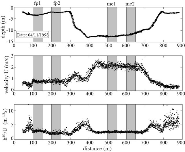
Figure 12. Measured depths (top graph), depth-averaged flow velocities (middle graph) and effective hydraulic resistance (bottom graph).
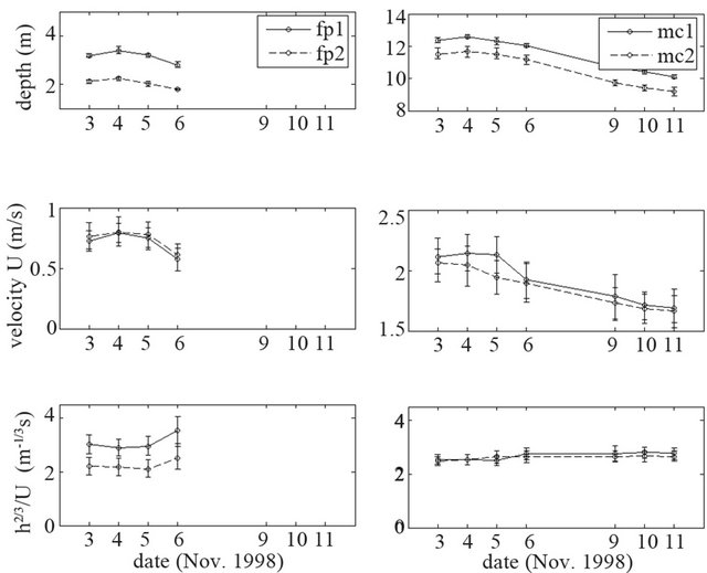
Figure 13. Time-dependency of the hydraulic characteristics within the averaged-regions in the floodplain (fp1 and fp2) and the main channel (mc1 and mc2, see Figure 12).
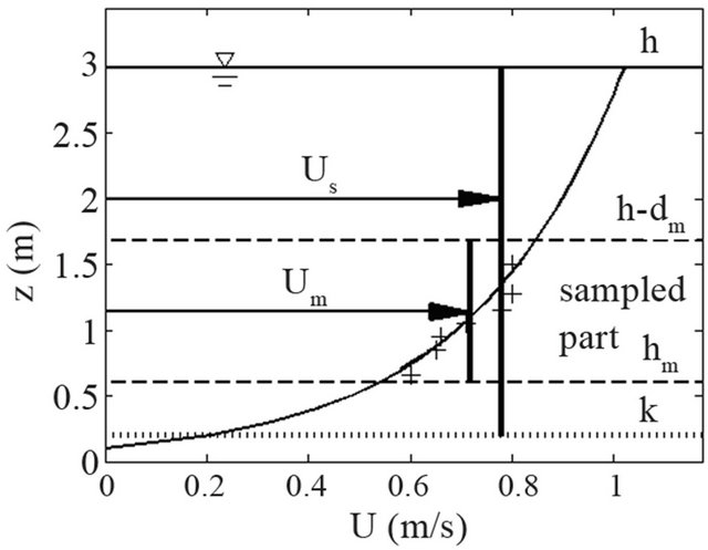
Figure 14. Sketch to illustrate the correction procedure of measured flow velocities.
surface dm=1.32 − 0.25/2 m. The steps in correcting the measured average velocity Um is as follows:
1) We assume that the flow field above the vegetation follows a vertical logarithmic velocity profile, with a first guess for the corresponding (Nikuradse) roughness height of kN = 0.1 m, which is a reasonable value for grass according to Van Velzen et al. [33].
2) The assumed profile is shifted vertically to fit the sampled flow velocity points (by minimizing least squares).
3) From the fitted profile, the average velocity in the surface layer Us is determined, assuming an initial value of the vegetation layer height of k = 0.06 m.
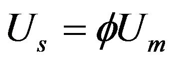
Figure 14 illustrates the procedure for correcting flow velocities in the surface layer. Effectively, the correction-procedure described above corresponds to multiplying the measured average flow velocity Um by a factor Φ:
 (7)
(7)
where
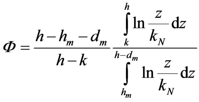 (8)
(8)
In Figure 15(a) the results after correcting flow velocities are shown. As expected, the corrections are largest for flow measurements in the shallower region fp2.
3.3. Comparison to Model Predictions
We compare the corrected flow velocities in the surface layer (Us), with values obtained with the simplified flow model proposed by Huthoff et al. [23]. If the depth of the surface layer (h − k) is more than three times the vegetation height, then the flow velocity in the surface layer is described by a simple scaling law (see Section 2.3):
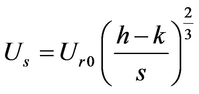 (9)
(9)
This expression can be rearranged to
 (10)
(10)
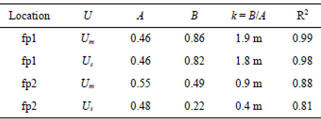
where A = (Ur0)3/2/s and B = Ak. The bottom graph in Figure 15 shows the measured and corrected averaged velocities, (Um)3/2 and (Us)3/2 respectively, set out against the flow depth h. For each data set also a best fit straight line is shown. Following Equation (10), the ratio B/A yields an estimate of k, which reflects the height of the drag dominated flow layer (or: the vegetation height). Table 1 gives an overview of these values.
The results in Table 1 show that for location fp2 the effective height of the drag-dominated flow layer is approximately k = 0.4 m, if using the corrected flow velocities Us. This value of 0.4 m is higher than expected for the floodplain under consideration (recall that we assumed 0.06 m in the correction procedure), but it is still acceptable for the type of vegetation that can be found in grassed floodplains. In contrast, for location fp1 an effective vegetation height of 1.8 m is found, which is unrealistically high given the nearly uniform vegetation characteristics in the floodplain meadow.
A closer inspection of conditions in the floodplain reveals that the flow depth at location fp1 is about 1.3 m
 (a) Measured and corrected velocities.
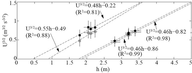 (b) Best fit for U3/2~h − k.
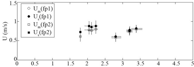
Figure 15. (a) Depth-averaged velocity U vs flow depth for locations fp1 and fp2 (filled symbols: corrected velocities); (b) Regression relations of U3/2 vs depth.
Table 1. Equivalent vegetation heights (k) reproduced from flow measurements and Equation (10).
deeper than at location fp2 (Figure 13), while the average flow velocities at these locations are nearly the same. It appears that in the deeper part of the floodplain water does not flow freely. Figure 16 shows the floodplain shortly after a flooding event in 2007, leaving behind a clearly confined pool at location fp1. Therefore, the larger depth at fp1 is a local topographic effect. Consequently, at fp1 we cannot assume (quasi-) uniform flow and therefore we cannot estimate the hydraulic roughness based on the average flow velocity and local flow depth. However, fp2 is not as much affected by local topographical variations, so for this location we can compare measured data to prediction using model Equations (1)- (6). Using the corrected average flow velocities at fp2 (Figure 15(a)), a vegetation height of k = 0.4 m (Table 1) and by adopting a vegetation spacing of s = 1 cm for grassed floodplains (see Van Velzen et al. [33]), Equation (9) yields an approximate characteristic velocity of Ur0 = 0.03 m/s. Next, if we use a channel slope of i = 10−4, which is a representative value for the considered part of the Rhine River [38], model Equations (1)-(6) give the Manning values as shown in Figure 17. It can be seen that for shallow flows Manning values can be as high as n = 0.15, while for flow depths h > 1.5 m values converge towards a constant value in the range 0.02 - 0.025. Also, the results for an assumed vegetation height of k = 0.06 m are shown, indicating that for grass-lined floodplains the vegetation height has only a minor effect on overall flow resistance for relatively deep flows (i.e. if h > 2 m). The predicted values in Figure 17 are slightly lower than those stated in Chow [35], who gives n = 0.030 +/− 0.005 for short grass in floodplains.
3.4. Discussion
We studied two cases of flows in natural vegetated waterways to investigate the bed roughness properties and to compare these to predictions from the vegetation roughness model proposed by Huthoff et al. [23]. Because of incomplete data sampling we were forced to make assumptions on the general shape of the velocity profiles, in order to obtain representative depth-averaged flow velocities. Despite the uncertainties associated with the obtained flow conditions it was shown that local topographic variations can have important impacts on the flow field, and that these localized effects can easily be misinterpreted as local changes in hydraulic roughness. Therefore, field flow measurements should be treated with extreme care if used to determine hydraulic parameters such as Manning’s roughness values.
Several studies have shown that remotely-sensed vegetation characteristics can be obtained with high enough accuracies to use them at as input for roughness parameterizations [32,39,40]. The vegetation roughness model proposed by Huthoff et al. [23] is based on such input
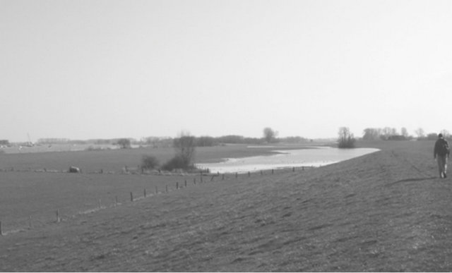
Figure 16. A clearly confined pool indicating a local depresssion in the floodplain (picture: F. Huthoff).
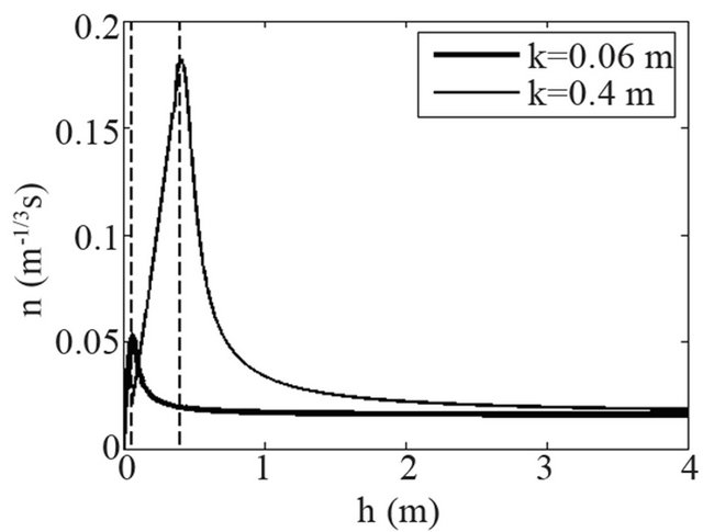
Figure 17. Manning’s n vs depth according to model Equations (1)-(6) adopting a velocity of Ur0 = 0.03 m/s in the vegetation layer and a vegetation spacing of s = 1 cm.
parameters (such as vegetation height and vegetation spacing), which gives opportunities for advanced inundation modeling techniques where measured vegetation characteristics are translated into effective roughness values.
In the current study, data limitations did not allow for an accurate field validation of the considered roughness model. However, it was shown that the model equations give predictions that are in the correct range and also agree with roughness values stated in the literature. For grass-lined floodplains, the model equations suggest that constant Manning values may be appropriate for wellsubmerged vegetation (h > 2 m), which has traditionally been the preferred approach in inundation studies (e.g. [41,42]). In contrast, for situations where the vegetation is just submerged, the model equations predict significant variations in Manning’s roughness values. The importance of these roughness variations for evolvement of floodplain inundations should be the topic of more focused research in the future.
4. Conclusion
In the case studies considered here, the waterways with submerged vegetation included predominantly grass species, having average stem heights that are easily an order of magnitude smaller than the flow depths. The vegetative roughness model proposed in Huthoff et al. [23] is consistent with measured flow velocities over such vegetation, predicting nearly constant Manning roughness values for well-submerged vegetation. In contrast, model equations predict that constant Manning’s roughness values are no longer appropriate when vegetation is just submerged. Future research should focus on the importance of vegetation roughness-changes under such conditions. Further, it was shown that topographical variations of the bed may have major impacts on local flow velocities, underlining that extreme care should be taken when using field data to estimate floodplain roughness coefficients.
5. Acknowledgements
This research is supported by the Technology Foundation STW, applied science division of NWO and the technology programme of the Ministry of Economic Affairs (Netherlands). We gratefully thank Aqua Vision for letting us use their data and Anne Wijbenga (HKV Consultants) for his valuable comments. We appreciate the help from Ivo Thonon and Chris Roosendaal (both Utrecht University), who assisted during the measurement campaign in Driel, and the help from Abe Klaas De Jong (HKV Consultants) and Blanca Pérez Lapeña (University of Twente), who assisted in producing the figures.
REFERENCES
- H. L. Cook and F. B. Campbell, “Characteristics of Some Meadow Strip Vegetation,” Agricultural Engineering, Vol. 20, No. 9, 1939, pp. 345-348.
- US Soil Conservation Service, “Handbook of Channel Design for Soil and Water Conservation,” United States Department of Agriculture, Annapolis, 1947.
- J. E. P. Green and J. E. Garton, “Vegetation Lined Channel Design Procedures,” Transactions of the American Society of Agricultural Engineers, Vol. 26, No. 2, 1983, pp. 437-439.
- C. A. M. E. Wilson and M. S. Horritt, “Measuring the Flow Resistance of Submerged Grass,” Hydrological Processes, Vol. 16, No. 13, 2002, pp. 2589-2598. HUdoi:10.1002/hyp.1049U
- R. Garcia Diaz, “Analysis of Manning Coefficient for Small-Depth Flows on Vegetated Beds,” Hydrological Processes, Vol. 19, No. 16, 2005, pp. 3221-3233. HUdoi:10.1002/hyp.5820U
- A. F. Lightbody and H. M. Nepf, “Prediction of Velocity Profiles and Longitudinal Dispersion in Emergent Salt Marsh Vegetation,” Limnology and Oceanography, Vol. 51, No. 1, 2006, pp. 218-228. HUdoi:10.4319/lo.2006.51.1.0218U
- J. C. Green, “Comparison of Blockage Factors in Modelling the Resistance of Channels Containing Submerged Macrophytes,” River Research and Applications, Vol. 21, No. 6, 2005, pp. 671-686. HUdoi:10.1002/rra.854U
- T. Sukhodolova, A. Sukhodolov and C. Engelhardt, “A Study of Turbulent Flow Structure in a Partly Vegetated River Reach,” In: G. Carravetta and D. Morte, Eds., River Flow, Vol. 1, 2004, pp. 469-478.
- J. K. Lee, L. C. Roig, H. L. Jenter and H. M. Visser, “Drag Coefficients for Modeling Flow through Emergent Vegetation in the Florida Everglades,” Ecological Engineering, Vol. 22, No. 4-5, 2004, pp. 237-248. HUdoi:10.1016/j.ecoleng.2004.05.001U
- J. Järvelä, “Flow Resistance of Flexible and Stiff Vegetation: A Flume Study with Natural Plants,” Journal of Hydrology, Vol. 269, No. 1-2, 2002, pp. 44-54. HUdoi:10.1016/S0022-1694(02)00193-2U
- Z. Shi and J. M. R. Hughes, “Laboratory Flume Studies of Microflow Environments of Aquatic Plants,” Hydrological Processes, Vol. 16, No. 16, 2002, pp. 3279-3289. HUdoi:10.1002/hyp.1102U
- C. A. M. E. Wilson, T. Stoesser, P. D. Bates and A. Batemann-Pinzen, “Open Channel Flow through Different Forms of Submerged Flexible Vegetation,” Journal of Hydraulic Engineering, Vol. 129, No. 11, 2003, pp. 847- 853. HUdoi:10.1061/(ASCE)0733-9429(2003)129:11(847)U
- A. Armanini, M. Righetti and P. Grisenti, “Direct Measurement of Vegetation Resistance in Prototype Scale,” Journal of Hydraulic Research, Vol. 43, No. 5, 2005, pp. 481-487. HUdoi:10.1080/00221680509500146U
- A. Murota, T. Fukuhara and M. Sato, “Turbulence Structure in Vegetated Open Channel Flow,” Journal of Hydroscience and Hydraulic Engineering, Vol. 2, No. 1, 1984, pp. 47-61.
- T. Tsujimoto, T. Kitamura and T. Okada, “Turbulent Structure of Flow over Rigid Vegetation-Covered Bed in Open Channels,” KHL Progressive Report 2, Kanazawa University, Kanazawa, 1991.
- D. Klopstra, H. J. Barneveld, J. M. van Noortwijk and E. H. van Velzen, “Analytical Model for Hydraulic Roughness of Submerged Vegetation,” The 27th International IAHR Conference, San Fransisco, 10-15 August 1997, pp. 775-780.
- D. Velasco, A. Bateman and V. De Medina, “A New Integrated Hydromechanical Model Applied to Flexible Vegetation in Riverbeds,” In: G. Parker and M. Garcia, Eds., River, Coastal and Estuarine Morphodynamics, 2005, pp. 217-227.
- D. G. Meijer and E. H. van Velzen, “Prototype-Scale Flume Experiments on Hydraulic Roughness of Submerged Vegetation,” The 28th International IAHR Conference, Graz, 22-27 August 1998, Article ID: D108.
- M. G. Khublaryan, A. P. Frolov and V. N. Zyryanov, “Modeling Water Flow in the Presence of Higher Vegetation,” Water Resources, Vol. 31, No. 6, 2004, pp. 668- 674. HUdoi:10.1023/B:WARE.0000046899.00404.baU
- Y. Shimizu and T. Tsujimoto, “Numerical Analysis of Turbulent Open-Channel Flow over Vegetation Layer Using a k-ε Turbulence Model,” Journal of Hydroscience and Hydraulic Engineering, Vol. 11, No. 2, 1994, pp. 57- 67.
- F. Lopez and M. H. Garcia, “Mean Flow and Turbulence Structure of Open Channel Flow through Non-Emergent Vegetation,” Journal of Hydraulic Engineering, Vol. 127, No. 5, 2001, pp. 392-402. HUdoi:10.1061/(ASCE)0733-9429(2001)127:5(392)U
- A. Defina and A. C. Bixio, “Mean Flow and Turbulence in Vegetated Open Channel Flow,” Water Resources Research, Vol. 41, No. 7, 2005, Article ID: W07006. HUdoi:10.1029/2004WR003475U
- F. Huthoff, D. C. M. Augustijn and S. J. M. H. Hulscher, “Analytical Solution of the Depth-Averaged Flow Velocity in Case of Submerged Rigid Cylindrical Vegetation,” Water Resources Research, Vol. 43, 2007, Article ID: W06413. doi:10.1029/2006WR005625
- N. S. Cheng, “Representative Roughness Height of Submerged Vegetation,” Water Resources Research, Vol. 47, No. 8, 2011, Article ID: W08517. HUdoi:10.1029/2011WR010590U
- C. Fischenich and S. Dudley, “Determining Drag Coefficients and Area for Vegetation,” Ecosytem Management & Restoration Research Program, US Army Corps of Engineers, Washington DC, 2000.
- F.-C. Wu, H. W. Shen and Y.-J. Chou, “Variation of Roughness Coefficients for Unsubmerged and Submerged Vegetation,” Journal of Hydraulic Engineering, Vol. 125, No. 9, 1999, pp. 934-942. HUdoi:10.1061/(ASCE)0733-9429(1999)125:9(934)U
- D. Sumner, J. L. Heseltine and O. J. P. Dansereau, “Wake Structure of a Finite Circular Cylinder of Small Aspect Ratio,” Experiments in Fluids, Vol. 37, No. 5, 2004, pp. 720-730. HUdoi:10.1007/s00348-004-0862-7U
- H. M. Nepf, “Drag, Turbulence, and Diffusion in Flow through Emergent Vegetation,” Water Resources Research, Vol. 35, No. 2, 1999, pp. 479-489. HUdoi:10.1029/1998WR900069U
- M. R. Raupach, “Drag and Drag Partition on Rough Surfaces,” Boundary-Layer Meteorology, Vol. 60, No. 4, 1992, pp. 375-395. HUdoi:10.1007/BF00155203U
- M. Fathi-Maghadam and N. Kouwen, “Nonrigid, NonSubmerged, Vegetative Roughness on Floodplains,” Journal of Hydraulic Engineering, Vol. 123, No. 1, 1997, pp. 51-57. HUdoi:10.1061/(ASCE)0733-9429(1997)123:1(51)U
- J. Järvelä, “Determination of Flow Resistance Caused by Non-Submerged Woody Vegetation,” Journal of River Basin Management, Vol. 2, No. 1, 2004, pp. 61-70. HUdoi:10.1080/15715124.2004.9635222U
- M. Straatsma, “3D Float Tracking: In Situ Floodplain Roughness Estimation,” Hydrological Processes, Vol. 23, No. 2, 2009, pp. 201-212. HUdoi:10.1002/hyp.7147U
- E. H. Van Velzen, P. Jesse, P. Cornelissen and H. Coops, “Stromingsweerstand Vegetatie in Uiterwaarden,” Report RIZA, Arnhem, 2003.
- B. C. Yen, “Open Channel Flow Resistance,” Journal of Hydraulic Engineering, Vol. 128, No. 1, 2002, pp. 20-39. HUdoi:10.1061/(ASCE)0733-9429(2002)128:1(20)U
- V. T. Chow, “Open-Channel Hydraulics,” McGraw-Hill, New York, 1959.
- J. M. Eij, “Verwerking van ADCP Stromingsmetingen rond de Pannerdensche Kop tijdens Hoogwater in November 1998,” Technical Report AV DOC 040211, Aqua Vision, Utrecht, 2004.
- A. W. E. Wilbers, “The Development and Hydraulic Roughness of Subaqueous Dunes,” Ph.D. Thesis, University of Utrecht, Utrecht, 2004.
- P. Y. Julien, G. J. Klaassen, W. B. M. Ten Brinke and A. W. E. Wilbers, “Case Study: Bed Resistance of Rhine River during 1998 Flood,” Journal of Hydraulic Engineering, Vol. 128, No. 12, 2002, pp. 1042-1050. HUdoi:10.1061/(ASCE)0733-9429(2002)128:12(1042)U
- D. C. Mason, D. M. Cobby, M. S. Horritt and P. D. Bates, “Floodplain Friction Parameterization in Two-Dimensional River Flood Models Using Vegetation Heights Derived from Airborne Scanning Laser Altimetry,” Hydrological Processes, Vol. 17, No. 9, 2003, pp. 1711-1732. HUdoi:10.1002/hyp.1270U
- M. W. Straatsma and M.J. Baptist, “Floodplain Roughness Parameterization Using Airborne Laser Scanning and Spectral Remote Sensing,” Remote Sensing of Environment, Vol. 112, No. 3, 2008, pp. 1062-1080. HUdoi:10.1016/j.rse.2007.07.012U
- A. P. Nicholas and C. A. Mitchell, “Numerical Simulation of Overbank Processes in Topographically Complex Floodplain Environments,” Hydrological Processes, Vol. 17, No. 4, 2003, pp. 727-746. HUdoi:10.1002/hyp.1162U
- V. Tayefi, S. N. Lane, R. J. Hardy and D. Yu, “A Comparison of Oneand Two-Dimensional Approaches to Modelling Flood Inundation over Complex Upland Floodplains,” Hydrological Processes, Vol. 21, No. 23, 2007, pp. 3190-3202. HUdoi:10.1002/hyp.6523U
NOTES
1A Green River is a secondary waterway that is only deployed for additional discharge if the discharge in the main river channel reaches a particular critical level.