Open Journal of Acoustics
Vol. 3 No. 2A (2013) , Article ID: 33442 , 11 pages DOI:10.4236/oja.2013.32A005
Effect of Biological Activity on Broadband Passive Fathometry
School of Engineering and Information Technology, University College, University of New South Wales, Canberra, Australia
Email: m.alam@adfa.edu.au
Copyright © 2013 Jahangir Alam et al. This is an open access article distributed under the Creative Commons Attribution License, which permits unrestricted use, distribution, and reproduction in any medium, provided the original work is properly cited.
Received April 19, 2013; revised May 19, 2013; accepted May 26, 2013
Keywords: Passive Fathometer; Bottom Profile; Bandwidth; Shrimp; Biological Noise
ABSTRACT
A passive fathometer can be formed by two vertically separated hydrophones. The depth can be estimated from the Green’s function between the hydrophones, which is calculated from the cross-correlation between ocean ambient noise fields received at those two hydrophones. The performance of the fathometer depends on the signal to noise ratio (SNR) and the resolution of the noise cross-correlation function. In a given environment, improved SNR and resolution of the cross-correlation function can be achieved through longer observations, more observation points, or increasing bandwidth. Long time averaging has been demonstrated, but requires that the channel be stationary over the averaging time. Hydrophone arrays are commonly used, but result in increased cost and complexity. Recent work shows that the SNR and resolution of the correlation function can also be improved by the use of the large bandwidth noise fields. This paper shows that the non-surface biological noise generated by marine animals, such as shrimp, is one of the major issues in the performance of such a broadband passive fathometer operating in shallow water. This noise tends to occur at higher frequencies. Frequencies at which significant non-surface biological noise is present cannot be used to improve fathometer performance. Consequently, the upper limit of frequencies that can be used in a passive fathometer is limited by the lower limit of the bandwidth occupied by the biological noise.
1. Introduction
The cross-correlation of wind generated surface noises between two or more hydrophones gives the estimation of the bottom profile of the ocean [1-4]. In the literature, the estimation of bottom profile using ocean ambient noise is called “passive fathometer” [2,4,5]. The estimate in the passive fathometer is based on the extraction of the Green’s Function (GF) from the ambient Noise Crosscorrelation Function (NCF) [2]. The GF between two points can be extracted from the derivative of the crosscorrelation between the Ocean Ambient Noise (OAN) received at those two points [6-8]. The better the estimate of the GF, the better the estimate in the passive fathometer. Two figures of merit for the estimates of the GF are the SNR and the resolution of the Cross-Correlation Function (CCF) [7,9-11].
One of the requirements for the improvement of the SNR and resolution of the CCF is that a large amount of OAN is needed [7,10,12]. There are a number of ways of collecting a large amount of OAN. It is shown that large averaging of the NCF is needed for the better estimation of the GF if the noise is recorded at two hydrophones [8,10,12-16]. But this takes long recording time. Another way of collecting large amounts of data is to use an array of hydrophones. In array processing, signals from different pairs of hydrophone are averaged together to improve the SNR of the correlation function [1,2,9]. The number of elements of the array can be increased to increase the SNR of the correlation function [2,5,10], but the array becomes physically larger. The increase in the number of elements does not increase the resolution of the correlation because the resolution is dependent on the bandwidth of the noise field [6].
However, array processing has been thought to be limited by the usable bandwidth of the noise field. That is, due to spatial aliasing the bandwidth cannot be larger than the design frequency of the array [2], even though the SNR and resolution can be improved by the increase of the bandwidth [9-11,17]. Some recent works show that the bandwidth can be increased by up to twice the design frequency without affecting the performance as a conesquence of spatial aliasing [5].
In this paper, it is demonstrated experimentally that, the usable bandwidth in the passive fathometer at shallow water is limited by the biological activities present in the ocean. This is because, dominant biological sounds are observed at shallow waters all around the world [18]. Experimental results show that due to the dominance of the strong shrimp sounds in the higher frequency band of the noise field, the upper band of the ocean ambient noise is not useful in the passive fathometer. However, the lower band of the OAN still satisfies the theoretical relationship between the performance of the passive fathometer and the bandwidth.
The rest of the article is organised as follows. Section 2 shows the theoretical demonstration of bottom profiling using cross-correlation of OAN. Section 3 demonstrates the experimental analysis of the broadband passive fathometer and the effect of biological activities in the ocean on it. Finally, Section 4 states the conclusion of the paper.
2. Theoretical Analysis
2.1. Cross-Correlation of Band-Limited Ocean Ambient Noise Fields
At frequencies of more than several hundred hertz and less than 20 kHz, most of the non-biological ambient noise in the ocean is generated at the ocean surface [19-23]. The main sources of the surface noise are the breaking waves and wind action on the surface of the ocean. Noise generated in the surface can be approximated as a sheet of noises just below the surface at a depth z′ [2]. It is also assumed that the noise creation rate and noise distribution is uniform. We consider a situation in which noise is recorded at two vertically separated hydrophones where hydrophones S1 and S2 are positioned at  and
and  in a cylindrical coordinate system. Since the hydrophones are vertically spaced,
 . The noise fields received at the hydrophones consist of direct signals and reflected signals from the seabed and surface. In the mathematical derivation, only the direct signals and first bottom reflected signals are considered to contribute in the noise fields because just the first bottom reflection is sufficient to describe the passive fathometer using cross-correlation. The geometry of the noise distribution and its bottom reflection image is shown in Figure 1 [2].
Figure 1 shows that a sheet noise is generated at z′ depth below the surface and a bottom image is generated at 2D − z′ depth from the surface where D is the depth of the seabed. The noise coming from all around the surface contributes to the noise fields received at two hydrophones S1 and S2.
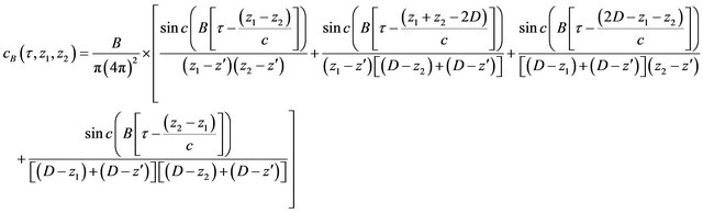
Now, the time domain cross-correlation function between the noise fields of bandwidth B received at S1 and S2 is expressed as [2,17].
The four sinc functions in Equation (1) represent four peaks generated due to the cross-correlation of coherent signals. The first sinc function represents the cross-correlation between the direct signals, the second and third sinc functions represent the cross-correlation between direct and reflected signals and the fourth sinc function represents the cross-correlation between the reflected signals. The amplitude and resolution of the sinc functions are dependent on the bandwidth of the recorded noise fields.
2.2. Depth Estimation from the Cross-Correlation
The depth of the seabed can be calculated from the delay difference between the direct and the bottom reflected paths received at two vertically separated hydrophones if the speed of sound is known [2,17]. This delay difference  can be estimated from the positions of the second and third correlation peaks in the cross-correlation shown in Equation (1).
 (1)
(1)
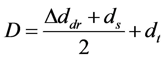
Now, the depth of the sea-bed D is given by
 (2)
(2)
where  can be measured from the NCF as
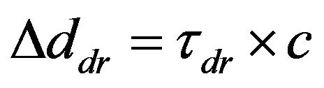 , and
, and  and
and  are known from the
Figure 1. Geometry of noise distribution and image formulation [2].
experimental setup. One of the main requirements of the correct depth estimation using two hydrophones is that the wind generated surface noises coming from the endfire region in the ocean surface need to be dominant in the ambient noise field. To achieve this requirement long averaging of the ambient noise is needed because of the randomness of surface noise both in time and space. An alternative means of overcoming the long averaging time is to use a linear array of hydrophones. The strong noises coming from directions other than the end-fire can be suppressed by steering the array towards the surface endfire region.
2.3. Relationship between SNR, Resolution and Bandwidth
Performance of the depth estimation of the ocean depends on how accurately the position of the correlation peak can be measured. The accuracy of the peak position in turns depends on the SNR and resolution of the correlation function. This is because the strength of the peak becomes stronger and the width of the peak becomes narrower with the increase of SNR and resolution of correlation function respectively.
The SNR of the CCF is defined as the ratio of the power of the correlation between coherent signals and that of uncorrelated signals. The relationship between the SNR of the cross-correlation and the bandwidth of the participating ocean ambient noise fields is [17]
 (3)
(3)
From Equation (3), we can say that the SNR of the cross-correlation of the noise signals recorded at two hydrophones is directly proportional to the bandwidth of the recorded signals.
The resolution of the CCF can be defined as the full width of the main lobe of the correlation peak [6]. A decrease in the peak width means an improvement in the resolution.
The resolution  of the CCF can be expressed as [6,17]
 (4)
(4)
Equation (4) shows that the resolution of the correlation improves with the increase of bandwidth.
2.4. Bandwidth Aliasing and Spatial
Spatial aliasing is a phenomenon of signal reception that occurs when a signal of a particular frequency is under-sampled in space by a set of receivers [24]. Spatial aliasing takes place when the spacing between the receivers is greater than half of the wavelength of the signal.
In a passive fathometer, an array of hydrophones is used to make use of beamforming to improve the performance. Therefore, in the broadband passive fathommeter, the effect of spatial aliasing needs careful consideration. This is because the aliased frequency components greater than the design frequency of the array also take part in the broadband passive fathometer. Although the direction finding of the narrowband signal is affected by spatial aliasing, in the broadband passive fathometer it should not be a problem. This is because in the vertical beamforming, the main lobes at zero degree angle fall on each other and the side lobes fall at different angles for different frequency components of the broadband data. Figure 2 shows the beamforming output for the broadband data (1 - 30 kHz) in the broadband passive fathometer.
In Figure 2, the strong main lobe at the angle of zero degree is observed compared to the weak side lobes. Therefore, we can say that the fathometer works in spite of the separation not satisfying spatial aliasing. The preliminary results of active fathometry by transmitting broadband linear chirp also show close agreement with the statement.
3. Experimental Analysis
The aim of the experiment is to validate the theory described in Section 2 and to demonstrate the effect of biological noise on the bottom profiling by recording broadband ocean acoustic ambient noise fields at vertical hydrophones. The experiment has been conducted at Jervis Bay, NSW, Australia on 13th of October 2011. An array of 4 hydrophones is used to record the broadband OAN. The experiment is conducted at different depths and different types of seabed such as sandy and rocky. In this article, analysis has been performed for the rocky bottom and about 15 meter depth of the sea bed to find out the effects of strong biological noise on passive fathometer, because the sound produced by the shrimps is dominant at shallow and rocky bottom areas.
3.1. Experimental Setup
A 4-hydrophone array is deployed underwater where the bottom hydrophone is at a depth of about 5.7 m from surface and the spacing between consecutive hydrophones is 50 cm. Bruel and Kjaer 8104 hydrophones are used in the array. The array is hung from a float in the surface using a 2.5 m long rope. Since the strength of OAN is low, a voltage preamplifier with 50 dB gain is used to amplify the ocean noise before recording. The preamplifier used in this experiment is RESON VP2000. Each 50 s data slot is recorded at a sampling rate of 192 ksps. The data acquisition device UA101 is used to capture the OAN. The UA101 has 10 input channels where four of them are used to record four channels of data simultaneously. The experimental setup is shown in Figure 3.
3.2. Passive Fathometer: Rocky Bottom and 15 m Depth
3.2.1. Noise Field
The noise field recorded at each hydrophone consists of the direct signal, bottom and sub-bottom reflected signals
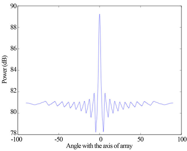
Figure 2. Output of the broadband vertical beamforming.
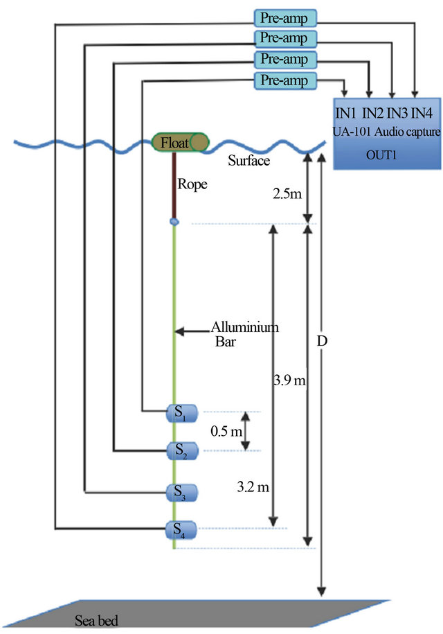
Figure 3. Experimental setup.
and surface reflected signals. The Power Spectral Density (PSD) of the noise fields recorded at S1 hydrophone is shown in Figure 4.
The PSD of the OAN and the internal noise of the system are shown by blue and red lines respectively in Figure 4. The PSD of the internal noise of the measurement system is almost flat having an absolute level of about −154 dBW/Hz. Figure 4 shows that the PSD of the OAN is not flat. At lower frequencies the power level of the recorded noise field is stronger than the higher frequencies. Therefore, the SNR of the noise field decreases with the increase of the bandwidth. In general, the PSD of the OAN falls at a rate of about 5 dB/octave towards higher frequencies which is in a good agreement with the OAN described in the literature [22,25,26]. An equalisation filter needs to be applied to the OAN to make the PSD of OAN flat before fathometer processing. The shipping and traffic noises are also expected to contribute at the strong low frequency (200 - 500 Hz) signals of the ambient noise. In passive fathometer processing, a high pass filter with cut-off frequency of 1 kHz is applied to the recorded noise fields to get rid of the strongest low frequency shipping noises. The surface noise field is expected to dominate over the frequency range from as low as 10 Hz to about 20 kHz in the OAN [20,22,23]. Therefore, a low pass filter with cut-off frequency of 20 kHz is also applied to the noise field to take the full band of the wind generated surface noise.
3.2.2. Cross-Correlation between Ocean Ambient Noise Fields
The cross-correlation of the ambient noise fields recorded at two vertically separated hydrophones is the basis of the passive fathometry applications. The crosscorrelation of the equalised and filtered (1 - 20 kHz) ambient noise fields received at S1 and S2 hydrophones is shown in Figure 5.
Since the depth at the experimental location is about 15 m measured by an active sonar and the two hydrophones S1 and S2 are about 4.2 and 4.7 m below the surface, the delay difference between the direct path at one hydrophone and the reflected path at other hydrophone is 14.07 ms according to the experimental setup of Figure 3.
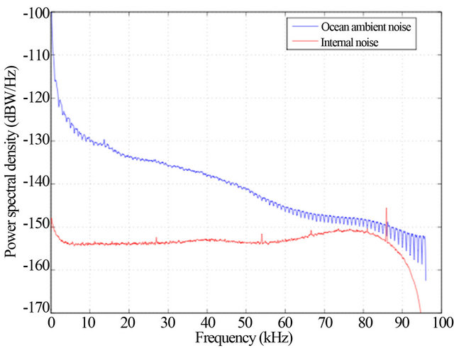
Figure 4. Power spectrum of the noise field recorded at S1 compared to the internal noise (red) of measurement system (colour online).
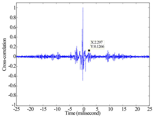
Figure 5. Cross-correlation of the equalised noise fields (1 - 20 kHz).
Hence correlation peaks are expected at 14.07 ms away in both sides of the correlation centre. In Figure 5, there are small correlation peaks at about 14.07 ms representing the depth of the ocean. But still the dominant peaks are generated at about 2.3, 9.36 and 11.9 ms away from the correlation centre, which have no relation with the estimation of the depth according to the experimental setup. Therefore, the small peaks representing the depth of the ocean cannot be distinguished from the other strong correlation peaks. These strong correlation peaks might be generated because of one of the following reasons:
1) A strong surface generated noise coming from the directions other than end-fire region.
2) Biological noise coming from all around the hydrophones.
3) Strong man-made noise generated at nearby places.
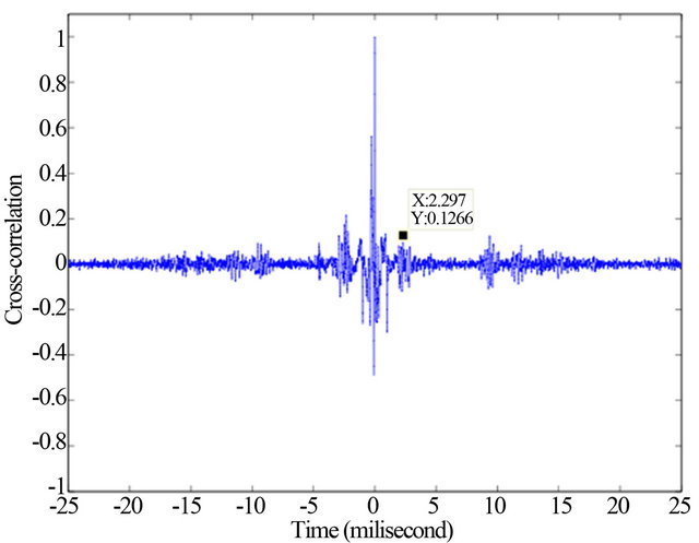
Since the OAN is recorded using an array of four hydrophones, comparing the cross-correlations of each pair of hydrophones, the direction from which the signals come can be determined. The cross-correlations between hydrophone pairs S1 and S2, S2 and S3, and S3 and S4 are shown in Figure 6.
The cross-correlation between S1 and S2 shown in Figure 6(a) generates a strong correlation peak at about 2.29 ms away from the correlation centre. In the crosscorrelation between S2 and S3 shown in Figure 6(b), this strong correlation peak moves away from the correlation centre and in the cross-correlation between S3 and S4 as shown in Figure 6(c), the same peak moves further away. Therefore, it can be said that since S1 and S4 are the top and bottom hydrophone of the array respectively, the noise source contributing the above mentioned correlation peak is coming from underneath the array. This is because the direct path signal from underneath the array comes later at S1 and earlier at S4 and the surface reflected signal comes earlier at S1 and later at S4. Therefore, we can say that the strong correlation peaks of Figure 6 are not generated by the surface generated noise, hence they do not give the estimation of the ocean depth.
To find out the reasons of generating strong correlation peaks at positions other than 14.07 ms, the time domain ocean noise fields need to be analysed. A 50 s slot of the OAN received by S1 is shown in Figure 7.
The filtered (1 - 20 kHz) noise field of Figure 7 includes the noise contribution from the wind generated noise at the surface and the biological activities in the ocean. This is because the frequency ranges of the wind generated noise and biological noise cover from less than 1 kHz to above 20 kHz and 200 kHz respectively. A number of sharp peaks are seen in the noise field of Figure 7. These dominant peaks might come from the biological activities of the marine animals because some of the ocean animals produce very sharp clicks [18,22,23],
 (a)
(a)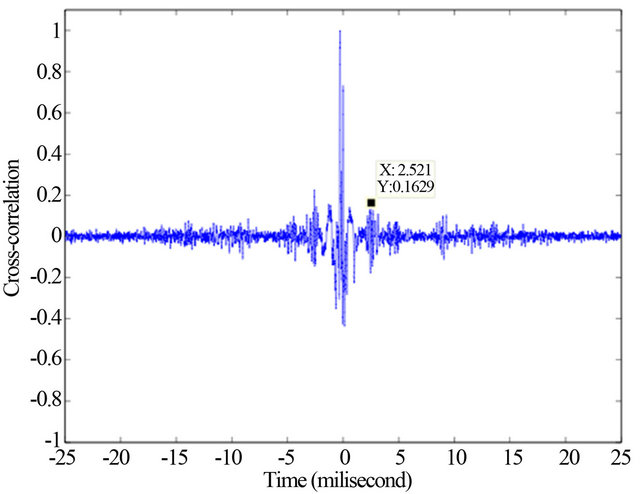 (b)
(b)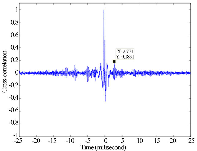 (c)
(c)
Figure 6. Cross-correlations of different pairs of hydrophones; (a) cross-correlation of S1 and S2; (b) cross-correlation of S2 and S3; (c) cross-correlation of S3 and S4.
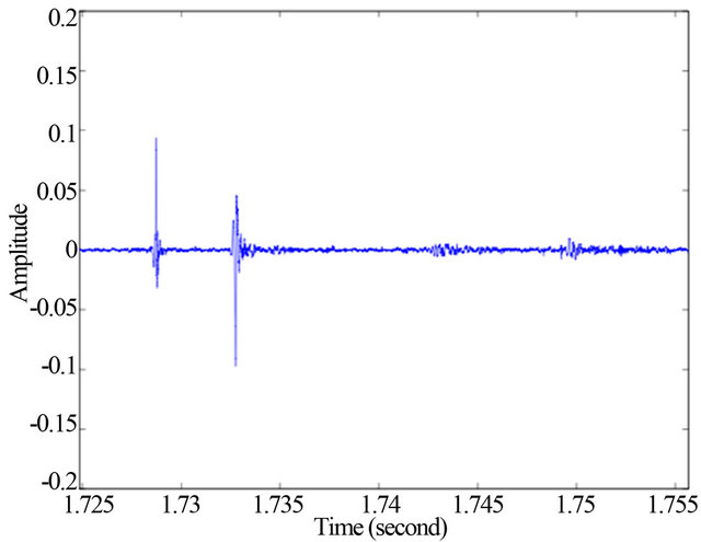
but further investigation is needed to confirm it. From Figure 7, it can be seen that the clicks are very frequent, but they are different in strength. A strong pulse of the noise field in the 2nd second of the recording is shown in Figure 8.
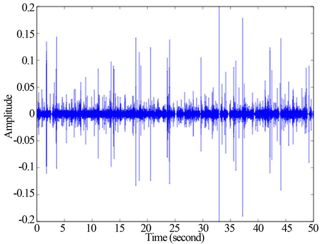
Figure 7. Ocean ambient noise received at hydrophone S1.
 (a)
(a)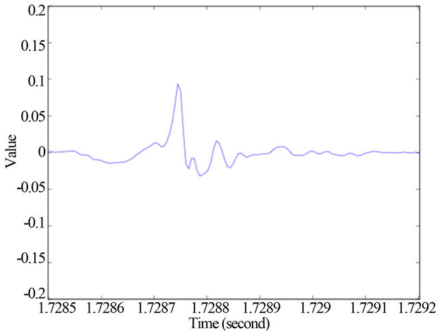 (b)
(b)
Figure 8. A strong click in the 2nd second of the noise field; (a) Pulse with consecutive reflections; (b) Direct path of the pulse.
Figure 8(a) shows a sharp peak with its consecutive reflections. Because of the sharp (intense) nature of the direct path signal of Figure 8(a), we can say that this signal is not coming from the wind generated surface noise. This is because the sound generated by the wind action of the surface is random in nature which can be approximated as a gaussian noise [27]. Figure 8 is not coming from the surface and they are too sharp to be the sound of whale breaching. Also the breaching of the humpback whales are not so frequent as is the case with the clicks in the noise field. The sperm whales also produce sound clicks but they mostly live in the deep water. Therefore, the sperm whales are probably not contributing to the clicks of the shallow water noise field of Jervis Bay. Bottlenose dolphins produce very sharp clicks of about 5 - 10 μs width and they might make sound in shallow water [18]. However, the clicks of dolphin are sporadic, therefore, should not be seen the clicks all over the noise field. Since the noise field of Figure 7 contains continuous clicks of sound, they are unlikely to be coming from the dolphin clicks. Although some of them might come from the dolphin because of the sporadic nature of the dolphin clicks.
Finally, shrimps produce almost the same types of click as the dolphin [18], the only obvious difference is that the sound made by shrimps are continuous because of the high density of these little animals in the ocean bottom. Therefore, there is a strong possibility that the clicks of the noise field are contributed by the sound of the shrimps. The time series of the sound produced by the shrimp from the previous literature is shown in Figure 9 to compare with the click shown in Figure 8.
Figure 9 shows the time series of the pulses from the snaps of the four individual shrimps in Sydney Harbour at Pyrmont [18]. The pulses shown in Figure 9 resemble the peak shown in Figure 8 with the main difference is that strong negative pulse is shown in the Jervis Bay noise field compared to Figure 9. The negative pulse is generated by the effect of applying high pass filter on the recorded noise field [6].
Therefore, we can infer that the sharp OAN over 1 to 20 kHz bandwidth is dominated by the shrimp clicks. Wind generated surface noise also contributes to that frequency band. The contribution of surface noise in the lower frequencies of the OAN is larger than that in the higher frequencies because of the downward trend of the PSD of the wind generated surface noise [22,25].
3.2.3. Effect of Snapping Shrimps on the Passive Fathometer
The second and third sinc functions of Equation (1) are used in the passive fathometer to estimate the depth of the seabed [17]. One of the necessary conditions behind the depth estimation is that most of the energy of the

Figure 9. Time series of the clicks produced by the shrimp [18].
noise field needs to come from the end-fire region of the surface. This condition holds for the OAN field at most of the places all around the world for long averaging time, because the wind generated surface noise due to the breaking waves is assumed to dominate over all other types of OAN in the frequency range of less than 1 kHz to about 20 kHz. However, the shallow water ambient noise field of Jervis Bay is not dominated by the sounds of the wave breaking, rather it is dominated by the sound of shrimps. Since the shrimps lie on the seabed, the mandatory condition of the dominant signal from the ocean surface does not hold in case of the OAN field of the Jervis Bay. Therefore, the broadband passive fathometer technique applied on the ambient noise field of Jervis Bay face challenges in estimation of the depth of the ocean. The geometry of the passive fathometer processing in the presence of strong shrimp noise is shown in Figure 10.
In Figure 10, a noise source A is positioned at the ocean bottom. A direct signal from A comes to the hydrophone S2 following AS2 path and a surface reflected path of the same signal comes to hydrophone S1 following ACS1 path. The cross-correlation between these two signals gives the delay difference between them, which is an estimation of the depth of the hydrophones, not the depth of the seabed. And it is caused because of the presence of the shrimps on the seabed.
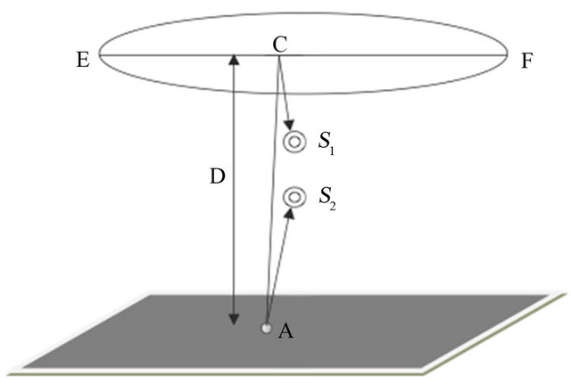
Figure 10. Effect of shrimp sound on passive fathometer.
Along with the strong biological sound, the comparatively weak wind generated signal is still present in the noise field, which creates weak correlation peaks corresponding to the depth of the ocean. However, it does not help in the estimation of the depth of the seabed because of the difficulty of identifying the correct correlation peak, in the presence of the strong correlation peak representing the depth of the hydrophones.
Another important condition of the passive fathometer is that the noise sources need to be uncorrelated. However, in case of biological noise sources this condition does not hold because a particular ocean animal produces a specific type of signal all the time and they are correlated. The sound clicks produced by the shrimps are almost the same, because the mechanism of the sound production of the shrimps is same. Therefore, not only a particular shrimp produce the same clicks but also the different shrimps produce almost the same types of clicks as shown in Figure 8. In the cross-correlation of these biological sounds, correlation peaks can be generated by any of the following cases 1) Cross-correlation between direct and reflected paths of a single click.
2) Cross-correlation between the clicks produced by the same shrimp at different times.
3) Cross-correlation between the clicks produced by the different shrimps.
Figure 5 showed only a centre part of the cross-correlation between the shrimp dominated noise fields which is sufficient to observe the correlation peaks generated by the cross-correlation between direct and reflected paths. The full cross-correlation of the 50 s of the noise fields is shown in Figure 11.
There are lots of strong correlation peaks far away from the centre of the cross-correlation. Therefore, the cross-correlation between the broadband OAN fields dominated by shrimp sound does not give correct estimation of the depth of the seabed. Rather it can be used to estimate something else such as location and density of the shrimp and the tracks of the AUVs which are not the scope of this article.
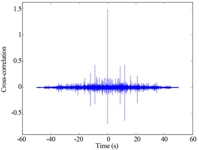
Figure 11. Cross-correlation between full length of 50 s noise fields.
3.2.4. Depth Estimation Using Ambient Noise of Lower Bandwidth
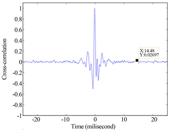
Because of the strong biological noise in the higher frequencies compared to the surface generated noise, only the lower band of the OAN may be used in the test of the passive fathometer. The passive fathometer by M. Siderius considers the frequency band of 200 to 1500 Hz along with Delay and Sum (DS) beam forming using an array of 32 elements to estimate the bottom profile of the ocean [2]. For the purpose of the comparison we also used the same lower frequency band in this analysis. A bandpass filter is applied very carefully on the received noise field. If the bandpass filter (200 - 1500 Hz) is applied directly to the noise field of the high bandwidth (96 kHz), the filter might be numerically unstable. So the received noise fields are low pass filtered and then down sampled at the ratio of 10:1 to make the effective bandwidth of the noise field 9.6 kHz and sampling rate 19.2 ksps. This helps to take the noise field of the frequency band of 200 to 1500 Hz. The cross-correlation between the equalised noise fields (200 - 1500 Hz) received at S1 and S2 is shown in Figure 12.
Figure 12 shows a correlation peak at about 14.48 ms which satisfies the depth of the experiment place. To make sure whether this peak is generated by the surface noise or not, the cross-correlations between different pair of hydrophones are evaluated and shown in Figure 13.
Figures 13(a)-(c) show the cross-correlation between S1 and S2, S2 and S3, and S3 and S4 respectively. The correlation peak at 14.48 ms away from the correlation centre generated by the cross-correlation between S1 and S2 hydrophones moves closer to the correlation centre in case of the other two correlations. In Figures 13(b) and (c), this peak is generated at 13.8 ms and 13.18 ms away from the correlation centre. Here the correlation peak moves closer when the cross-correlation involves the downward hydrophones in the array as opposed to the
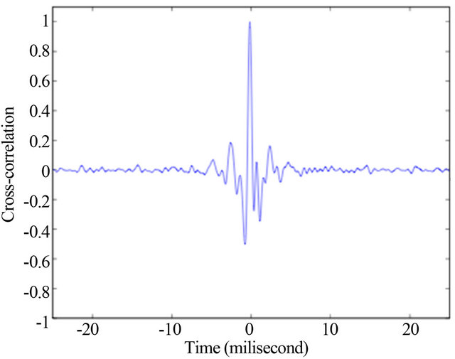
Figure 12. Cross-correlation of the equalised noise fields (200 - 1500 Hz) at hydrophones S1 and S2.
cross-correlations shown in Figure 6. Therefore, we can say that the correlation peak at about 14.48 ms is generated by the cross-correlation between the wind generated surface noise, hence this peak gives estimation of the depth of the seabed. Because of using the lower band of noise field and the cross-correlation between only two hydrophones, SNR of the peak is poor. To improve the SNR, two stages of the DS beamforming are applied on the cross-correlations between every pair of hydrophones.
After applying the DS beamforming using four hydrophones of the array, the resultant cross-correlation between the equalised noise fields (200 - 1500 Hz) is shown in Figure 14.
Figure 14 shows the evidence of the correlation peak at about 14.5 ms with good SNR, which corresponds to the path difference of 21.75 m. Now using Equation (2), depth of the rocky bottom can be estimated as:
where  m,
m,  m and
m and  for the reference hydrophone S1 in the DS beamforming.
At the beginning of the experiment the depth of the experiment was measured as 15 m using an active sonar which shows good agreement with the passive estimation of the depth. However, slight variation might be observed due to the uneven rocky seabed and drifting of the hydrophones with the ocean current.
From the experimental analysis described here, we can say that using the power equalisation, lower frequency band of the OAN gives the estimation of the depth of the seabed in the passive fathometer. Although the large bandwidth OAN is processed to improve the SNR and resolution of the estimation in the passive fathometer, the noise fields at higher frequencies do not contribute to the passive fathometer due to the dominance of shrimp noises at shallow Australian water.
 (a)
(a)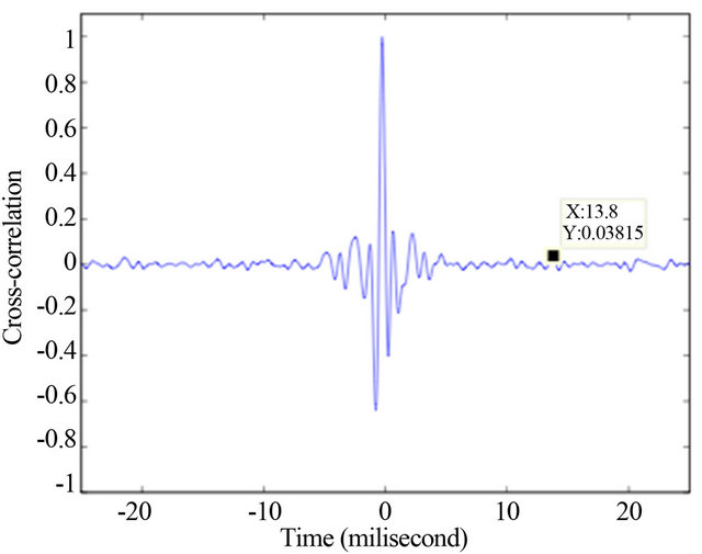 (b)
(b)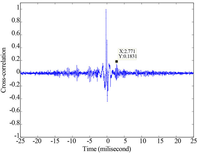 (c)
(c)
Figure 13. Cross-correlations of equalised noise fields (200 - 1500 Hz) at different pairs of hydrophones; (a) Cross-correlation of S1 and S2; (b) Cross-correlation of S2 and S3; (c) Cross-correlation of S3 and S4.
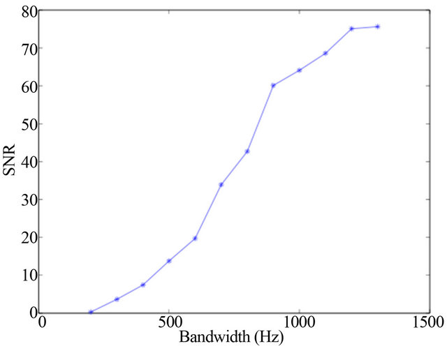
However, still the lower frequency band of 200 to 1500 Hz shows the consistency with the theoretical relationship of SNR and resolution of the CCF with the bandwidth of the OAN as shown in Section 2. The rate of increase of the SNR and resolution with respect to the bandwidth of the noise field is shown in Figure 15.
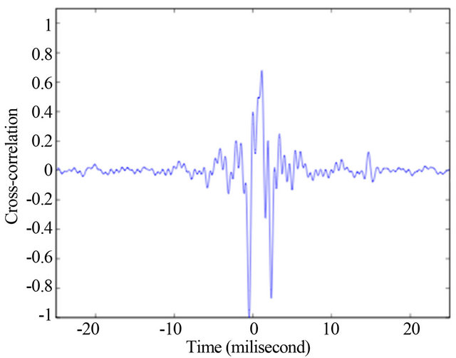
Figure 14. Cross-correlation between the equalised noise fields (200 - 1500 Hz) after DS beamforming using a 4-hydrophone array.
 (a)
(a)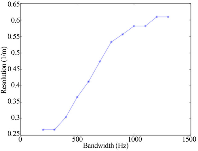 (b)
(b)
Figure 15. Experimental SNR and resolution of the correlation function with respect to bandwidth; (a) SNR vs bandwidth; (b) Resolution vs bandwidth.
The SNR is calculated as the ratio of the power of the correlation peak generated at about 14.5 ms and variance of the correlation noise generated in between 25 ms to 50 ms of Figure 14. The resolution is the calculated as the width (zero-crossing) of the correlation peak generated at about 14.5 ms in the cross-correlation.
Figure 15 shows that the relationship between SNR, resolution and bandwidth is broadly consistent with the theories of Equations (3) and (4). The rate of increase is slow both at lower and higher bandwidths over the frequency range of 200 to 1500 Hz. This is because of the effect of bandpass filter on the lower band signal and the dominancy of shrimps on the higher band.
4. Conclusion
This paper demonstrates the effect of biological activities on the broadband passive fathometer which states that performance of the passive fathometer is affected with the increase of the bandwidth of OAN. The experimental results from Jervis Bay, NSW, Australia show that in the shallow water bottom profiling, usable bandwidth of the ocean ambient noise is limited by the broadband sounds produced by the shrimps. This is because, at higher frequencies of ambient noise, the sound generated by the wave breaking and the shrimps overlap and dominated by the later. Since the sound generated by the shrimp does not contribute to the bottom profiling, upper band of the ocean ambient noise is not useful in the passive fathometer. However, still the lower band (200 - 1500 Hz) of the noise field from Jervis Bay satisfies the theoretical relationship between SNR, resolution and bandwidth in the passive fathometer. To overcome the performance degradation of the broadband passive fathometer due to the sound produced by the shrimps, active sonar can be used in the bottom profiling in the shallow water.
REFERENCES
- C. H. Harrison, “Sub-Bottom Profiling Using Ocean Ambient Noise,” Journal of the Acoustical Society of America, Vol. 115, No. 4, 2004, pp. 1505-1515. doi:10.1121/1.1645854
- M. Siderius, C. H. Harrison and M.B. Porter, “A Passive Fathometer Technique for Imaging Seabed Layering Using Ambient Noise,” Journal of the Acoustical Society of America, Vol. 120, No. 3, 2006, pp. 1315-1323. doi:10.1121/1.2227371
- C. H. Harrison and M. Siderius, “Bottom Profiling by Correlating Beam Steered Noise Sequences,” Journal of the Acoustical Society of America, Vol. 123, No. 3, 2008, pp. 1282-1296. doi:10.1121/1.2835416
- J. Traer, P. Gerstoft and W. S. Hodgkiss, “Ocean Bottom Profiling with Ambient Noise: A Model for the Passive Fathometer,” Journal of the Acoustical Society of America, Vol. 129, No. 4, 2011, pp. 1825-1836. doi:10.1121/1.3552871
- P. Gerstoft, W. S. Hodgkiss, M. Siderius, C. H. Huang, and C. F. Harrison, “Passive Fathometer Processing,” Journal of the Acoustical Society of America, Vol. 123, No. 3, 2008, pp. 1297-1305. doi:10.1121/1.2831930
- S. A. Albahrani, M. R. Frater and E. H. Huntington, “Linearly Filtered Estimation of the Time-Domain Greens Function from Measurements of Ambient Noise,” Journal of the Acoustical Society of America, Vol. 124, No. 5, 2008, pp. 2699-2701. doi:10.1121/1.2981049
- K. G. Sabra, P. Roux and W. A. Kuperman, “Emergence Rate of the Time-Domain Greens Function from the Ambient Noise Cross-Correlation Function,” Journal of the Acoustical Society of America, Vol. 118, No. 6, 2005, pp. 3524-3531. doi:10.1121/1.2109059
- S. E. Fried, W. A. Kuperman, K. G. Sabra and P. Roux, “Extracting the Local Greens Function on a Horizontal Array from Ambient Ocean Noise,” Journal of the Acoustical Society of America, Vol. 124, No. 4, 2008, pp. 183- 188. doi:10.1121/1.2960937
- K. G. Sabra, P. Roux, A. M. Thode, G. L. DSpain, W. S. Hodgkiss and W. A. Kuperman, “Using Ocean Ambient Noise for Array Self Localization and Self-Synchronization,” IEEE Journal of Oceanic Engineering, Vol. 30, No. 2, 2005, pp. 338-347. doi:10.1109/JOE.2005.850908
- P. Roux, W. A. Kuperman and the NPAL Group, “Extracting Coherent Wave Fronts from Acoustic Ambient Noise in the Ocean,” Journal of the Acoustical Society of America, Vol. 116, No. 4, 2004, pp. 1995-2003. doi:10.1121/1.1797754
- R. Snieder, “Extracting the Greens Function from the Correlation of Coda Waves: A Derivation Based on Stationary Phase,” Physical Review, Vol. 69, No. 4, 2004, 8 Pages.
- R. L. Weaver and O. I. Lobkis, “Fluctuations in Diffuse Field Correlations and the Emergence of the Greens Function in Open Systems,” Journal of the Acoustical Society of America, Vol. 117, No. 6, 2005, pp. 3432-3439. doi:10.1121/1.1898683
- O. I. Lobkis and R. L. Weaver, “On the Emergence of the Greens Function in the Correlations of a Diffuse Field,” Journal of the Acoustical Society of America, Vol. 110, No. 6, 2001, pp. 3011-3017. doi:10.1121/1.1417528
- R. L. Weaver and O. I. Lobkis, “Elastic Wave Thermal Fluctuations, Ultrasonic Waveforms by Correlation of Thermal Phonons,” Journal of the Acoustical Society of America, Vol. 113, No. 5, 2003, pp. 2611-2621. doi:10.1121/1.1564017
- J. Ricket and J. Claerbout, “Acoustic Daylight Imaging via Spectral Factorization: Helioseismology and Reservoir Monitoring,” The leading Edge, Vol. 18, No. 8, 1999, pp. 957-960. doi:10.1190/1.1438420
- N. M. Shapiro and M. Campillo, “Emergence of Broadband Rayleigh Waves from Correlations of Ambient Seismic Noise,” Geophysical Research Letters, Vol. 31, 2004, Article ID: L07614.
- J. Alam, M. R. Frater and E. H. Huntington, “Improving Resolution and Snr of Correlation Function with the Increase in Bandwidth of Recorded Noise Fields during Estimation of Bottom Profile of Ocean,” Sydney, 2010.
- D. H. Cato and M. J. Bell, “Ultrasonic Ambient Noise in Australian Shallow Water at Frequencies up to 200 khz,” Technical Report, DSTO Materials Research Laboratory, Urbana, 1992.
- K. Wapenaar, J. Thorbecke and D. Draganov, “Relations between Reflection and Transmission Responses of ThreeDimensional Inhomogeneous Media,” Geophysical Journal International, Vol. 156, No. 2, 2004, pp. 179-194. doi:10.1111/j.1365-246X.2003.02152.x
- M. R. Liewen and W. K. Melvile, “A Model of the Sound Generated by Breaking Waves,” Journal of the Acoustical Society of America, Vol. 90, No. 4, 1991, pp. 2075-2080. doi:10.1121/1.401634
- G. B. Deane, “Sound Generation and Air Entrainment by Breaking Waves in the Surf Zone,” Journal of the Acoustical Society of America, Vol. 102, No. 5, 1997, pp. 2671- 2689. doi:10.1121/1.420321
- G. M. Wenz, “Acoustic Ambient Noise in the Ocean: Spectra and Sources,” Journal of the Acoustical Society of America, Vol. 34, No. 12, 1962, pp. 1936-1956. doi:10.1121/1.1909155
- D. H. Cato and R. D. McCauley, “Australian Research in Ambient Sea Noise,” Acoustics Australia, Vol. 30, No. 1, 2002, pp. 13-20.
- M. J. Hinich, “Processing Spatially Aliased Arrays,” Journal of the Acoustical Society of America, Vol. 64, No. 3, 1978, pp. 792-794. doi:10.1121/1.382044
- V. O. Knudsen, R. S. Alford and J. W. Emling, “Underwater Ambient Noise,” Journal of Marine Research, Vol. 7, 1948, pp. 410-429.
- V. O. Knudsen, R. S. Alford and J. W. Emling, “Survey of Underwater Sound, Report No. 3, Ambient Noise,” Office of Scientific Research and Development, National Defence Research Committee, Washington DC, 1944.
- F. B. Jensen, W. A. Kuperman, M. B. Porter and H. Schmidt, “Computational Ocean Acoustics,” American Institute of Physics, New Work, 1994.