Open Journal of Acoustics
Vol.2 No.1(2012), Article ID:17798,10 pages DOI:10.4236/oja.2012.21005
High Frequency Roughness Scattering from Various Rough Surfaces: Theory and Laboratory Experiments
1Passive Acoustics, Superior National School of Advanced Techniques of Brittany, Brest, France
2LMA, French National Centre for Scientific Research, Marseille, France
3GIPSA-LAB, SIGMAPHY, National Center for Scientific Research, Grenoble, France
4The Naval Hydrographic and Oceanographic Service, Brest, France
Email: virginie.jaud@gmail.com
Received December 19, 2011; revised January 18, 2012; accepted January 30, 2012
Keywords: Bistatic Scattering; Tank Experiment; Anisotropic and Isotropic Roughness
ABSTRACT
The scattering strength of isotropic and anisotropic rough surfaces was experimentally and theoretically investigated for high frequencies about 500 kHz. Emphasis was placed on studying the response from three two-dimensional rough surfaces which roughness was either isotropic (characterized by a gaussian distribution) or anisotropic (characterized by a modified-sine surface). Theoretical predictions rely on the first-order small slope approximation either including a Gaussian structure function or a quasi-periodic structure function. The combination of true data and theoretical results indicates the importance of taking into account the anisotropy of a surface in a scattering prediction process. It is shown that the scattering strength varies a lot depending on the propagation plane. In the longitudinal direction of ripples, scattering strength is mostly in the specular direction, whereas in the transversal direction of the ripples, the scattering strength is spread in a very different way related to the particular features of the ripples, with several maxima and minima independent of the specular direction. Contrary to the isotropic surface, the scattering strength from an anisotropic rough surface is modified from one propagation plane to another, which explains why the entire rough surface should be taken into account without any simplification as it is often seen when dealing with scattering models. Compared to such a surface, positions of the emitter and of the receiver are naturally significant when measuring scattering strength.
1. Introduction
Acoustics scattering from the ocean bottom is a subject of interest for many remote sensing acoustic sensing marine activities, such as seabed classification, or ecosystem habitat mapping [1,2]. To these purposes, high frequency tools, as single beam or multibeam echosounders or side scan sonars, are used to assess the bottom roughness and improve the knowledge of the environment [3,4]. However if such systems can generally provide a detailed image of the bottom, the relationship between the acoustic measurements and the physical parameters of the bottom strongly depend on the type of environment, and in particular on the type of bottom roughness. To gain more insights into scattering phenomena, different well known models can be used. One of the most common models is based on the Kirchhoff approximation [5,6] and need large curvature of the rough interface compared to the acoustic wavelength. Another widely used model is based on the small perturbation method [7,8] and is valid only when the small-scale roughness is smaller than the acoustic wavelength. Then a composite model has been derived to avoid limitations of the two previous scattering models [9,10], but is only valid for monostatic cases and isotropic rough seafloors. Jackson and coworkers [10-12] have modified the monostatic method to obtain a bistatic model which only works for isotropic surfaces. This model was used by Choi et al. [13,14] for comparing theory with real data obtained from their measurements above ripple field. Nevertheless their comparisons showed that the orientation of the measurement plane compared to the direction of the ripples has a great effect on the scattering, the scattering strength distribution being very different from one propagation plane to another over the ripples. Thus they conclude on the need of considering the anisotropic state of a surface into the scattering process. To take into account both an isotropic or an anisotropic seabed, the small slope approximation, originally developed by Voronovich [15], is interesting since it allows considering various rough interfaces via the structure function. This method has been elaborated as a unifying method able to reconcile small perturbations method and Kirchhoff approximation [16].
Theoretical expressions have been developed at different orders by Thorsos and Broschat in [17,18] without taking into account quasi-periodic seafloors and further studied by Gragg et al. and Jackson et al. [19,20] in the case of isotropic interfaces. In this paper, the main concern is to better understand how an anisotropic rough surface can impact the acoustic propagation and scattering. The small slope approximation allows us to modify directly the height statistics, either by using true measurements of a rough surface [21] or by using theoretical model via the height covariance function of the seabed to describe its roughness. This modelling approach differs from many computations where anisotropy is directly implemented in the scattered field. The advantage of including the roughness straightforwardly in the model has to be tempered by the unique limitation of SSA of first order which is that the elevation slopes have to be small enough to avoid shading, particularly at very grazing angles. However, this is an asset compared to other scattering models where limitations are more numerous. This paper whose main goal is to study the effect of a twodimensional anisotropic rough surface on the scattering strength response using the small slope approximation is organized as follows. Section 2 describes the scattering problem and shows in theory the differences between predictions of scattering from an isotropic rough surface and from an anisotropic rough surface using the first order small slope approximation. In Section 3, tank experiments, which configurations are similar to the theoretical ones studied in Section 2, are reported. Scattering data from an isotropic surface and from an anisotropic surface are obtained for different angular configurations and from three different rough plates. We finally discuss, in section 3, the effect of the relief combining true data and simulated scattering strength results.
2. Modelling of Scattering Strength with SSA-1
2.1. SSA-1 Modelling
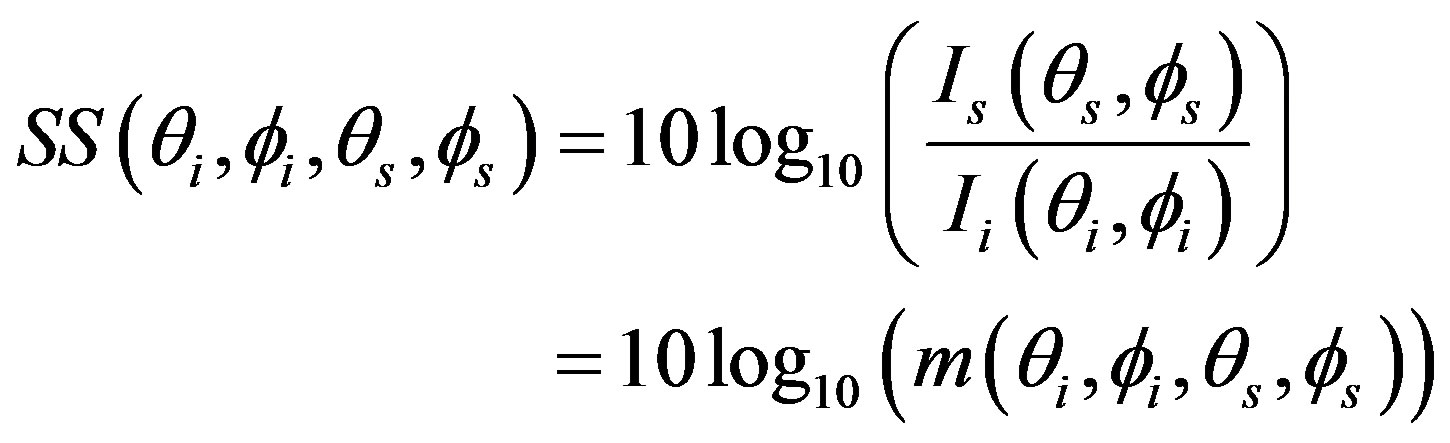
The scattering problem is depicted in Figure 1 and is analyzed trough the scattering strength, SS, which is defined in decibel (dB) as:
 (1)
(1)
where Ii is the incident intensity, Is is the scattered intensity and m is the dimensionless scattering coefficient. The latter parameter represents how the acoustic wave is scattered from the rough surface (ref. at 1 m-distance over a 1 m2 surface).
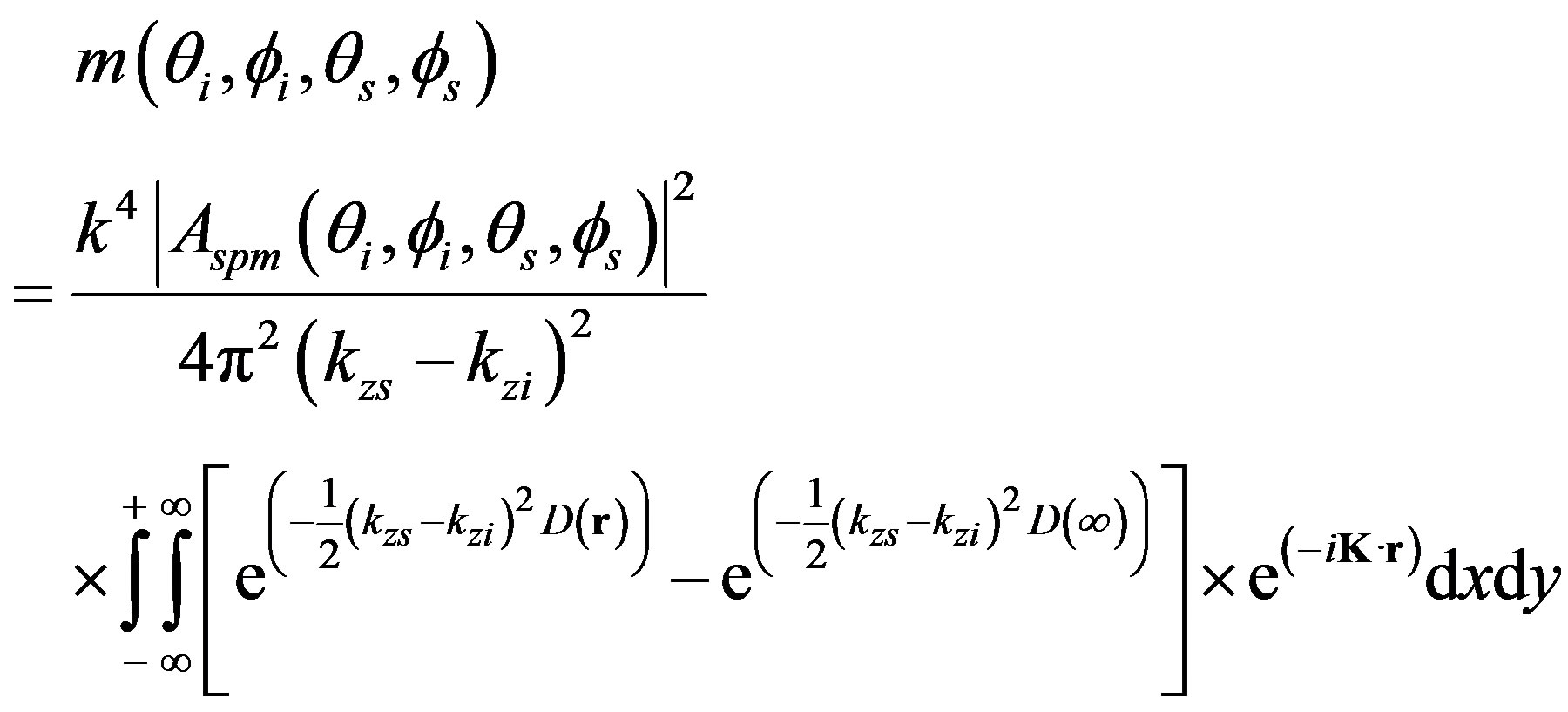
In this study, m is evaluated by using the first-order small slope approximation [12,15,17,19] and is written as:
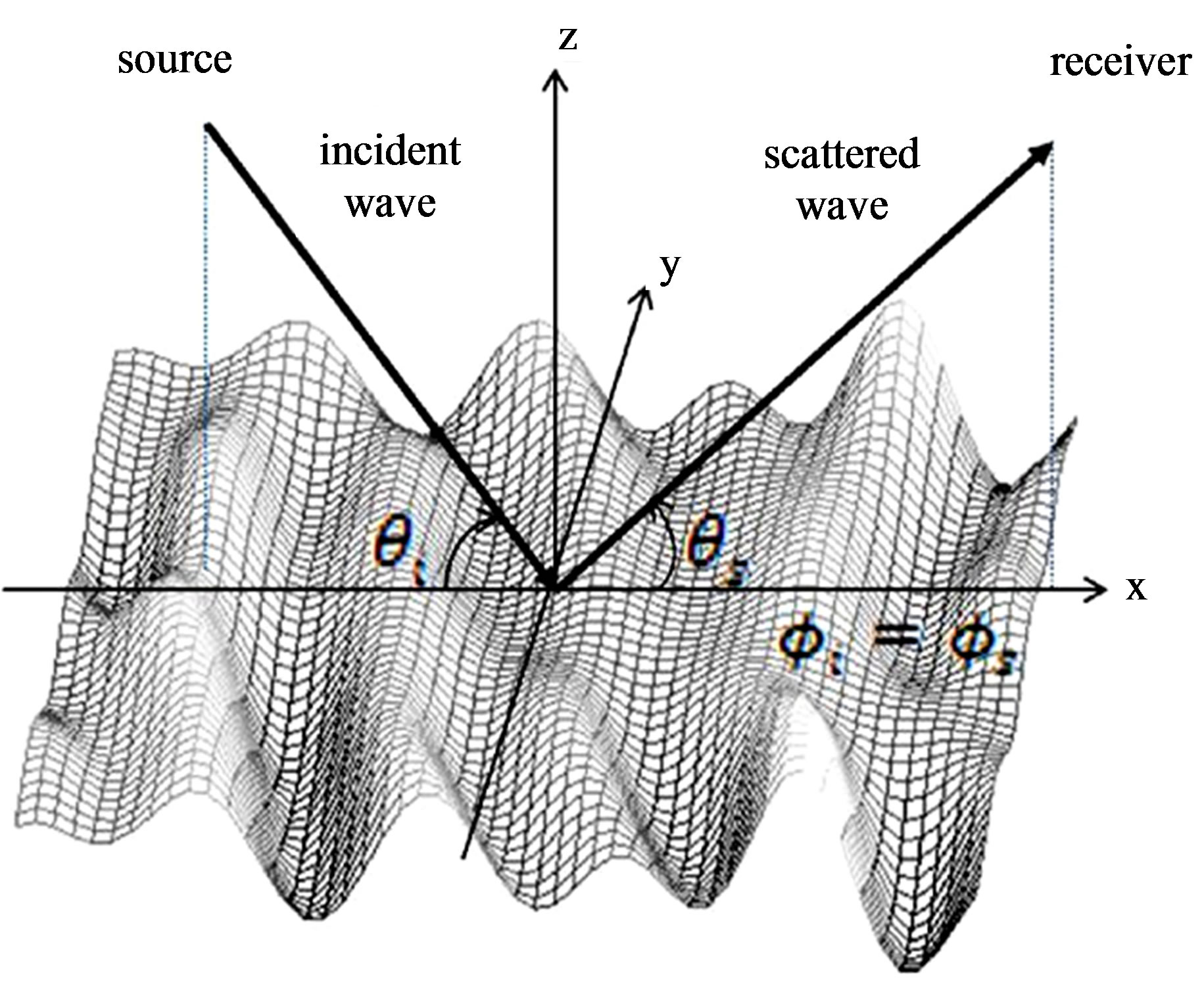
Figure 1. Geometry of the scattering problem with the grazing incident angle , the grazing scattered angle
  and the azimuth scattered angle
  equal to the azimuth incident angle
  (incident and scattered waves in a same plane).
 (2)
(2)
where 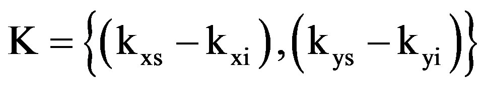 is the wavevector difference,
  is the position on the (x, y)-plane and D(r) is the structure function. The incident wave is defined by its grazing incident angle
  whereas the scattered wave depends on the grazing scattered angle
 . For this study we assume that the emitter and the receiver are always in the same plane, thus the azimuth angles are equal for both incident and scattered waves
  and
and . Figure 2 shows examples of various angular configurations of interest in this paper.
Scattering from sediment volume and multiple scattering are not considered in this paper. The losses of energy due to transmission into the sediment (from homogeneous or stratified seafloor) are considered through  which depends on the plane wave reflection coefficients and on the incident and scattered waves [12,22]. The sediment is defined as a fluid or as an elastic medium, thus
  is respectively related to the expression found in [12] or in [23]. The SSA model is parametrized with either a structure function based on a Gaussian distribution (see Equation (3)) or on a structure function based on a sine function (see Equation (4)).
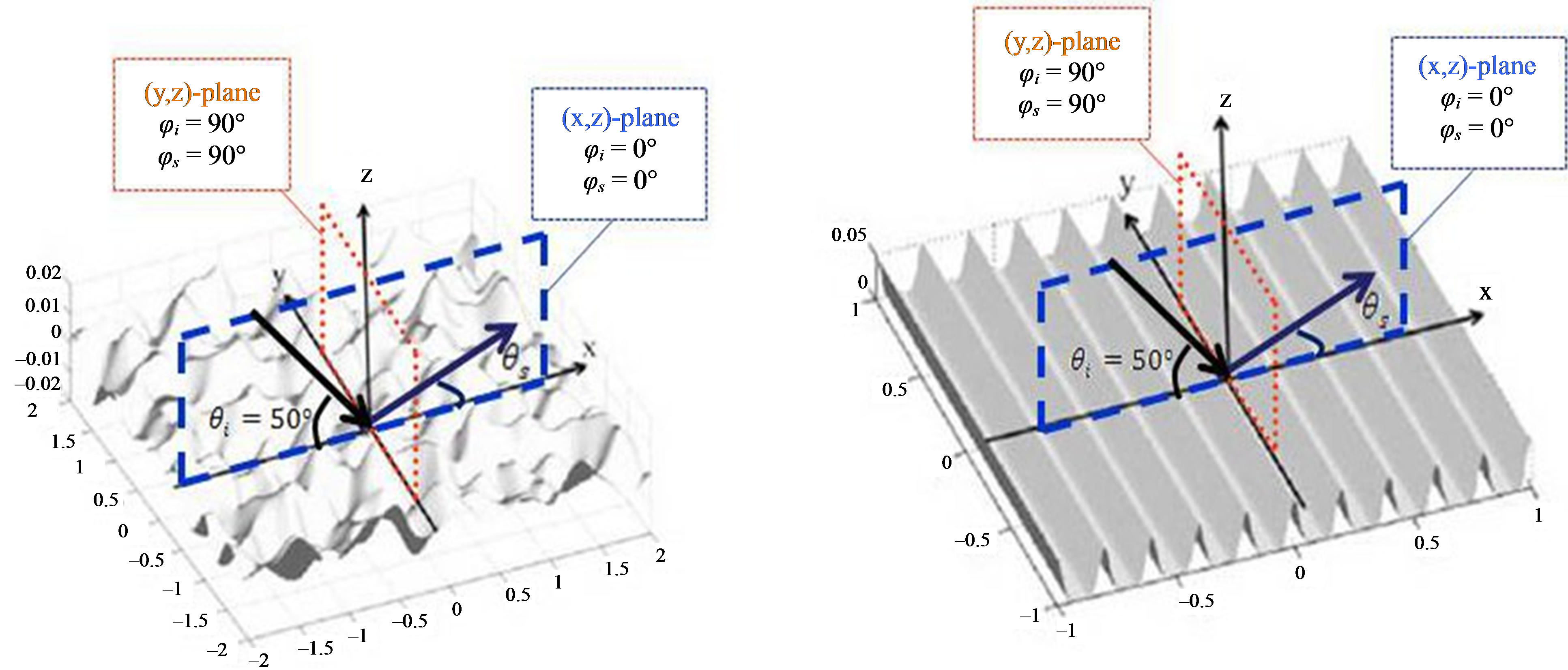
Figure 2. Angular configurations for different cases of interest: (left) configuration for an isotropic surface as a function of the scattered angle ; (right) configuration for an anisotropic surface as a function of the scattered angle
 .
.
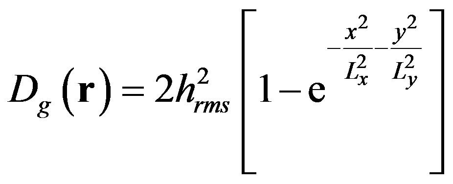 (3)
(3)
The structure function Dg is used either to model an isotropic surface or an anisotropic surface, depending on the values applied to the correlation lengths, Lx and Ly, respectively in the x and y directions. To deal with a part of periodicity and directionality of an interface, such as sandy ripples, we suggest another structure function, Dp which is based on a sine function.
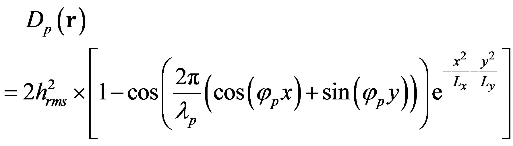 (4)
(4)
The structure function Dp is used to model a rough surface with periodic features, thus the surface is anisotropic and respects few but mandatory statistical properties such as the second-order stationary of the surface and its ergodicity. Surfaces based on this structure function are called ripples hereafter. The terms φp and λp are respectively the angle for the direction of the periodic sine shape and the wavelength of the sine function. The correlation lengths Lx and Ly allow to get a rough surface with periodic features more or less disordered.
2.2. Scattering Strength Predictions from an Isotropic Surface with SSA-1
We address first the case of an isotropic Gaussian seabed. This case may be considered as a reference case for further comparisons with anisotropic cases. Figure 3 shows
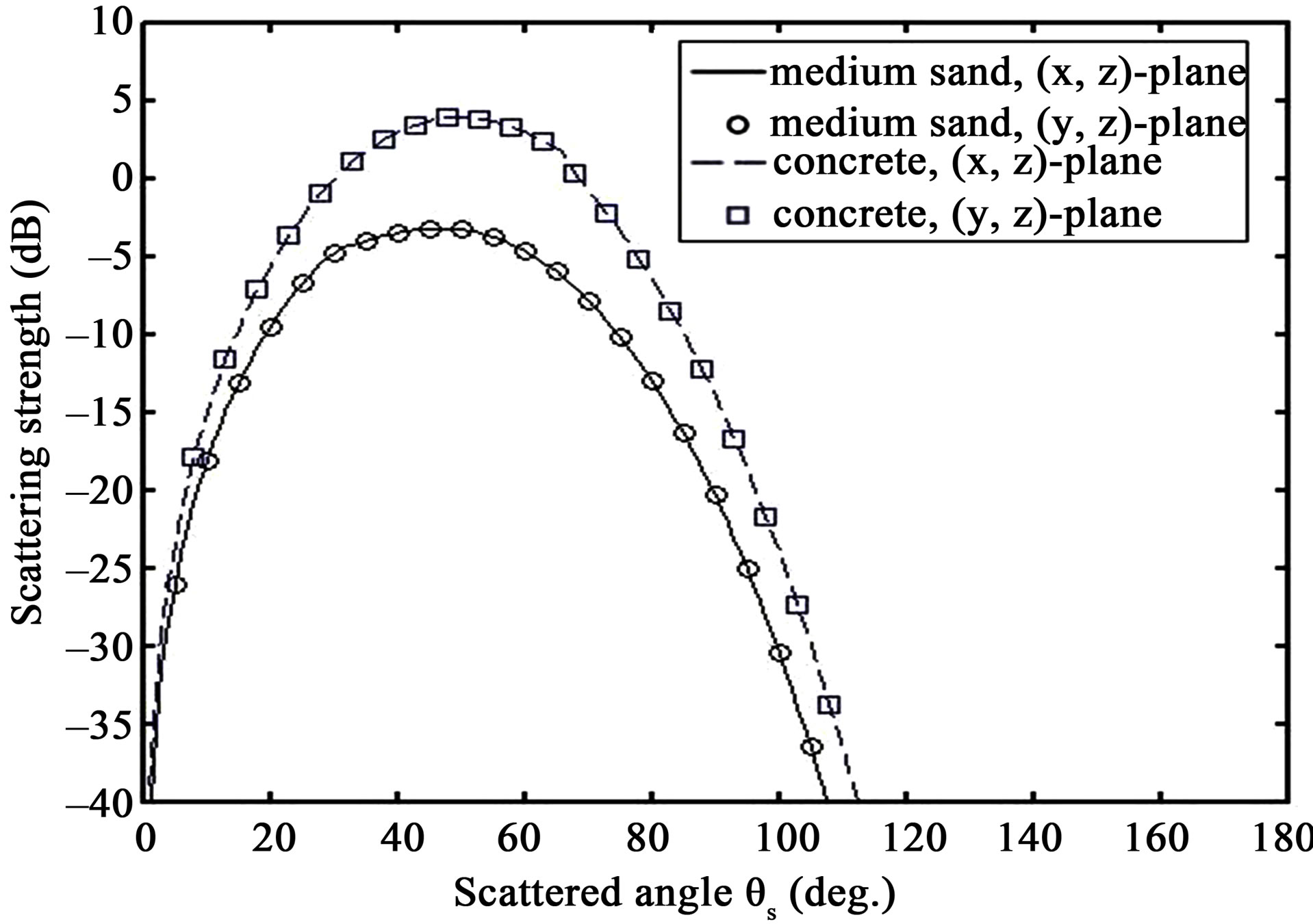
Figure 3. Prediction of scattering strength, SS, as a function of grazing scattered angle , for
, for ; (dashed line and squares) medium sand parameters; (full line and circles) concrete parameters; (dashed line and full line) propagation plane in the (x, z)-plane with
 ; (circles and squares) propagation plane in the (y, z)-plane with
 .
.
the scattering strength, SS, as a function of the scattered angle for a grazing incident angle  into two different propagation planes, the (x, z)-plane with
 , being perpendicular to the (y, z)-plane with
 , as it shown in Figure 2. The rough surface is isotropic and is based on a Gaussian distribution. The dimensions are similar to the rough plate, Plate 1, used in experiment and described in the experimental section (see Section 3). Its height deviation is between –1.5 mm and +1.5 mm with a zero-mean reference plane. The correlation lengths in both x-direction and y-direction are similar with
 . The frequency of the incident wave is 500 kHz, corresponding to a wavelength of 3 mm. Two different seabed sediments (with the same roughness parameters given previously) are also used for the predictions, one being defined by the parameters of a usual marine sediment [11,12] (medium sand with a sound velocity 1770 m/s of and a mass density of 1845 kg/m3) and the other one being based on the parameters of the concrete used in the experiment in Section 3 (mass density 2160 kg/m3 and compressional sound speed 3700 m/s).
For medium sand and concrete, the scattering strength predicted in the (x, z)-plane is obviously similar to the one predicted in the (y, z)-plane. The highest value for both medium sand and concrete is found for , thus in the specular direction and decreases for scattered angles lower and higher than the angle
 . The main difference between the two types of sediment is the global level which is higher for concrete since losses due to absorption are less important. In any case, the scattering strength distribution is as a function of the propagation plane since scattering strength is spread similarly in the (x, z)-plane and in the (y, z)-plane.
2.3. Scattering Strength Predictions from an Anisotropic Surface with SSA-1
The predictions from an anisotropic plate are now considered to analyze the effect of anisotropic roughness on the scattering strength distribution as a function of grazing scattered angle . Figures 4 and 5 show the scattering strength as a function of the grazing scattered angle
  for a grazing incident angle
 . The rough surface is a quasi-periodic anisotropic seabed and is based on a sine structure function as described by Dp(r) which expression is given by Equation (4). The dimensions are close to the ones of Plate 2 and of Plate 3, used in the experiment in Section 3. The peak-to-peak height is 3 mm, the wavelength of the surface is
 , the orientation angle, φp, is set to zero and the correlation lengths Lx and Ly, needed for Dp(r) are set to 10 m which is much longer than the surface wavelength (
 ). The frequency of the incident wave is 500 kHz, thus a wavelength of 3 mm. Three different anisotropic plates are used to simulate the scattering strength, one being defined by the parameters of a usual sediment [11,12] (medium sand with a sound velocity 1770 m/s of and a mass density of 1845 kg/m3), the second one based on the parameters of concrete used in the experiment (mass density 2160 kg/m3 and compressional sound speed 3700 m/s). The last case is based on wax parameters (mass density 720 kg/m3 and compressional sound speed 1722 m/s), used as well in the experiment in Section 3. One should notice that the wax shows a sound speed similar to a sandy sediment but a mass density much lower than the water, that may have an effect on
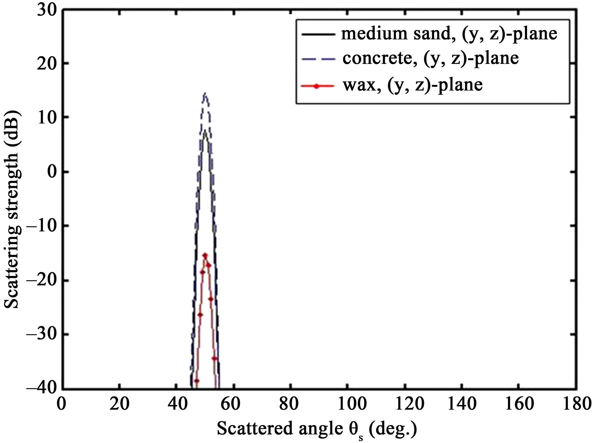
Figure 4. Prediction of scattering strength, SS, as a function of grazing scattered angle , for
, for , in the (y, z)- plane with
 ; (full line) medium sand parameters; (dashed line) concrete parameters, (red line with dots) wax parameters.
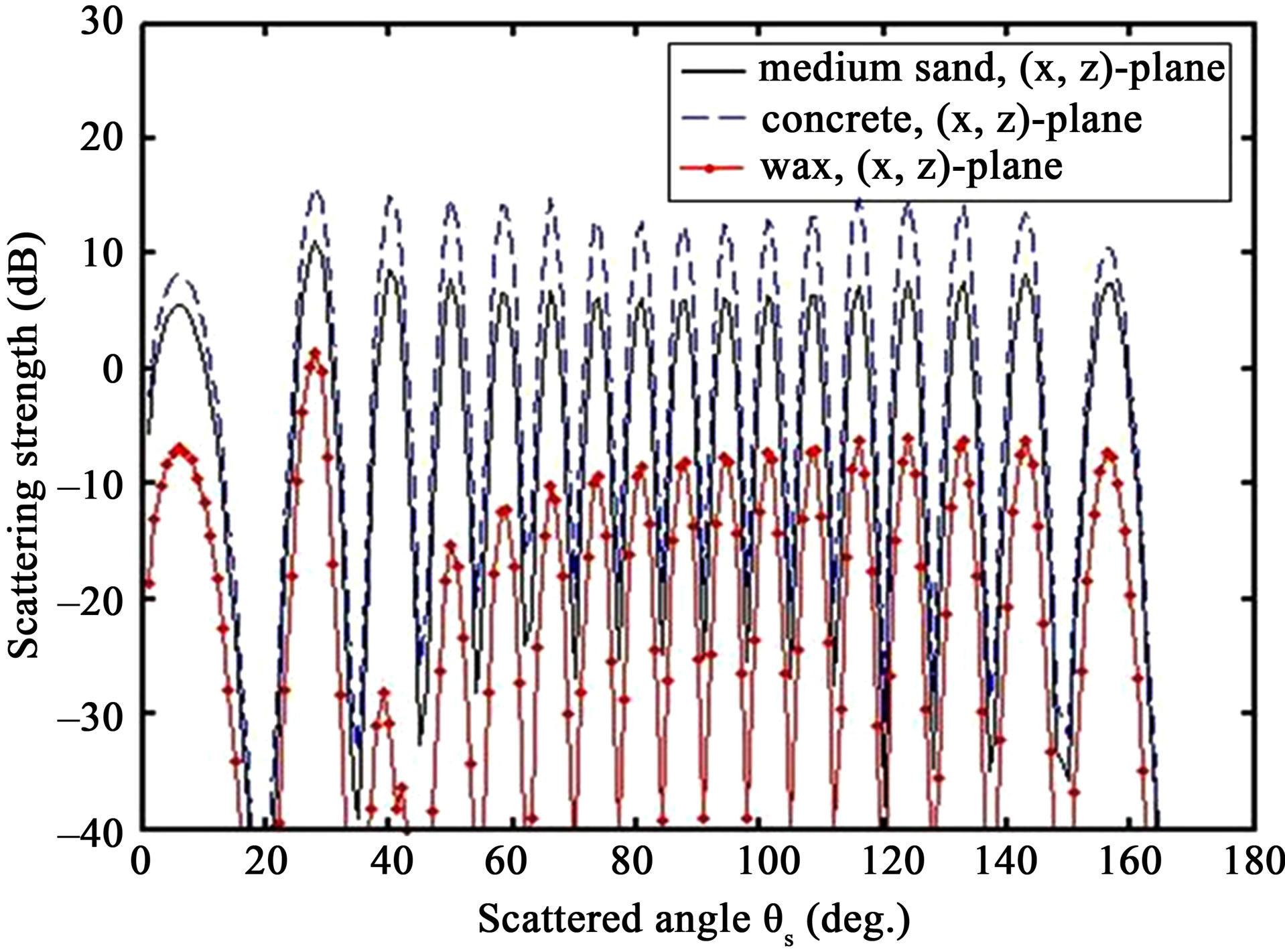
Figure 5. Prediction of scattering strength, SS, as a function of grazing scattered angle , for
, for  in the (x, z)-plane with
 ; (full line) medium sand parameters; (dashed line) concrete parameters, (red line with dots) wax parameters.
the scattering strength since its prediction is also related to sediment losses into the seafloor.
Figure 4 shows the predictions of the scattering strength, SS, for the three types of surface (full line for medium sand, dashed line for concrete and red line with dots for wax) for a propagation plane in the (y, z)-plane,  , thus in the longitudinal direction of the sine distributed relief (see Figure 2 for the propagation plane and its angular configuration). For each test case, the maximum value is found in the specular direction for
 . The highest value, about 15 dB, is obtained for the concrete sediment, then medium sand shows a lower level close to 10 dB. The lowest one, about –15 dB, is obtained for the wax. The angular band around the maximum value for each sediment case is about few degrees 10 dB below the maximum value, thus the scattering strength falls down straightaway.
Figure 5 shows the scattering strength, SS, as a function of scattered angle  for a propagation plane in the (x, z)-plane,
  , thus in the transverse direction of the sine distributed relief (see Figure 2 for the propagation plane and its angular configuration). The scattering dynamic is completely different from the previous simulations in the (y, z)-plane and strong variations are obtained for the different rough surfaces under test. The highest values are obtained in case of a concrete seafloor, then from a medium sediment and finally from the wax seafloor. For each type of sediment, seventeen peaks are found. These peaks vary between 9 dB and 15 dB, between 5 dB and 10 dB and between –30 dB and 2 dB, respectively for a sediment made of concrete, medium sand and wax. In the scattered angular band
 , the maximum levels are very similar from one peak to the other, particularly for a seafloor made of concrete or medium sand and not for the wax sediment. The latter test case shows a much lower value for the scattered angle around 40˚ (around –30 dB). This is due to the particular characteristics of this surface which properties are far from a real seafloor and are not accurately processed by the scattering model. This explains why expected scattering behaviors, taking into account losses into the sediment, are easily defined for concrete and medium sand. The scattered angular band at –10 dB below each maximum values is only about decibels (equal or less than 5˚) and is probably related to the dimensions of the quasi-periodic surface and particularly to the relationship between the acoustic wavelength and the height and surface wavelength.
The most important results from Figures 4 and 5 are that the scattering strength predicted in a plane is different from transversal to longitudinal directions. In the longitudinal direction, the roughness seems smoother in the transversal direction where the sine shape is of importance. Furthermore the scattering strength distribution is clearly related to the shape and dimensions of the surface compared to the acoustic wavelength and the angular position of the source and receiver. To validate the main results obtained with the small slope approximation, tank experiments are performed and are presented in the following section.
3. Scattering Data in a Tank
3.1. Experimental Set-Up
The acoustic experiments were performed at a water tank facility of Laboratoire de Mécanique et d’Acoustique (LMA, Marseille, France) in May 2011. The tank dimensions were about 290 cm × 140 cm and the measured sound speed in the water was about 1478 m/s at a temperature equal to 18.6˚C.
Three different plates were tested. Two plates, so-called Plate 1 and Plate 2, were made of concrete and were about 30 cm × 30 cm in sizes, with a mean thickness of 6 cm. Plate 1 was isotropic, its height deviation was between –1.5 mm and +1.5 mm with a zero-mean reference plane. The correlation lengths in x-direction and y-direction were similar with . Plate 2 was anisotropic, the wavelength of the sine relief was 2.5 cm and the peak-peak height was 3 mm. Both plates have been built to represent desired structure functions. The isotropic one was based on a Gaussian distribution and the anisotropic one was based on a modified sine function which bottom is larger than the top of the sine. The mass density has been calculated for both plates, based on a sample of concrete whose weight and dimensions were known, and is about 2160 kg/m3. The compressional sound speed in the sediment has been measured using a sample of concrete and on time measurements for a signal going through this sample. The sound speed was approximately 3700 m/s. Figure 6 (top) shows a close-up photo of Plate 1 and of Plate 2.
The third plate, Plate 3, is very similar in dimensions to Plate 2, but is made of wax which properties are 1722 m/s and 720 kg/m3 respectively for compressional sound speed and mass density. These parameters have acoustically been measured on a sample of wax which dimensions and weight were known. This plate is perfectly homogeneous and is shown on the close-up photo in Figure 6 (bottom).
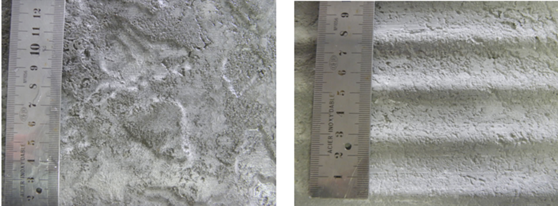
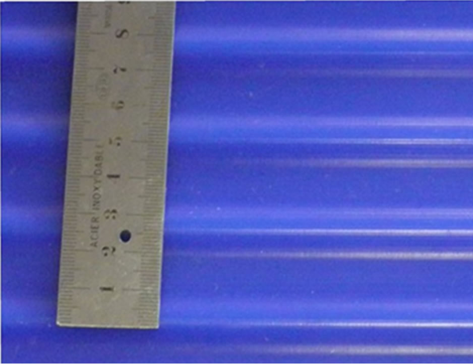
Figure 6. (top left) Plate 1, close-up photo on the isotropic plate (30 cm × 30 cm) made of concrete; (top right) Plate 2, close-up photo on the anisotropic plate (30 cm × 30 cm) made of concrete. The ruler is graduated in centimeters; (bottom) Plate 3, close-up photo on the anisotropic plate (34.5 cm × 34.5 cm) made of wax. The ruler is graduated in centimeters.
The transmitted signal was a short pulse of main frequency 500 kHz (bandwidth 300 kHz at –3 dB), thus a 3 mm-wavelength emitted with a Panametrics-v301 transducer whose directivity function is similar to the directivity of a circular piston of 26 mm-diameter with a beam width of . Acoustic signal recordings were sampled at 32 mhz with a 64 bit resolution. The receiver was Panametrics-v301 transducer which directivity was similar to the one used for emitting the signal.
Figure 7 shows the temporal and spectral characteristics of the transmitted signal, obtained from a reference measurement (calibration) between the emitter and the receiver without any plate in between. The distance between the emitter and receiver being the same during the experiments, the correction of the losses due to the distance is automatically taken into account for each measurement.
In the results presented in the following, the measured scattering strength has been calculated for different sets of angles (incident and scattered waves) from the measured time series by computing its Fourier transform. The scattering coefficient is obtained from Equation (5)
 (5)
(5)
where  is the amplitude of the reference signal (calibration) at a frequency f,
  is the amplitude obtained for a particular position of the transmitter
 , for a particular position of the receiver
  and at a frequency f. The results are presented for f = 500 kHz. The scattering strength is obtained in dB from the scattering coefficient
  v.
v.

Figure 7. (top) Time response of the 500 kHz transducer from the reference measurement; (bottom) spectrum of the 500 kHz transducer from the reference measurement.
The main angular configuration is described in Figure 1. The measurements have been done for an emitter with different positions with ,
,  and
and . For each incident grazing angle, the receiver was moved automatically from
  to
to  every 1˚. The emitter and the receiver were always in the same plane and measurement have been performed into two different planes, in the (x, z)-plane and in the (y, z)-plane as described in Figure 2, for each rough plate. Depending on the angle, the insonification area varied from about a 12 cm-diameter (transducer perpendicular to the plate) to a 25 cm-diameter (transducer oblique to the plate), assuming a distance of 1 m between the transducer and the plate.
For each angular configuration and each rough plate, the experiment has been processed several times (a minimum of 5 times up to a maximum of 10 times depending on the rough plate and on propagation plane of interest) and data are shown through their median. One should notice that from one measurement to the other, in the same configuration, data were extremely similar, with a maximum standard error of 0.1 dB.
3.2. Measured Results: From an Isotropic Surface (Plate 1)
The scattering strength measured as a function of scattered strength for the isotropic plate is shown in Figure 8 and in Figure 9 for an incident wave  and
and  respectively. For both angular configurations the data are measured such as the emitter and the receiver are in a plane, either the (x, z)-plane or the (y, z)-plane as it is described in Figure 2.
In Figure 8, the maximum value appears around , which is the specular direction and the minimum values are found for values of the scattered angle
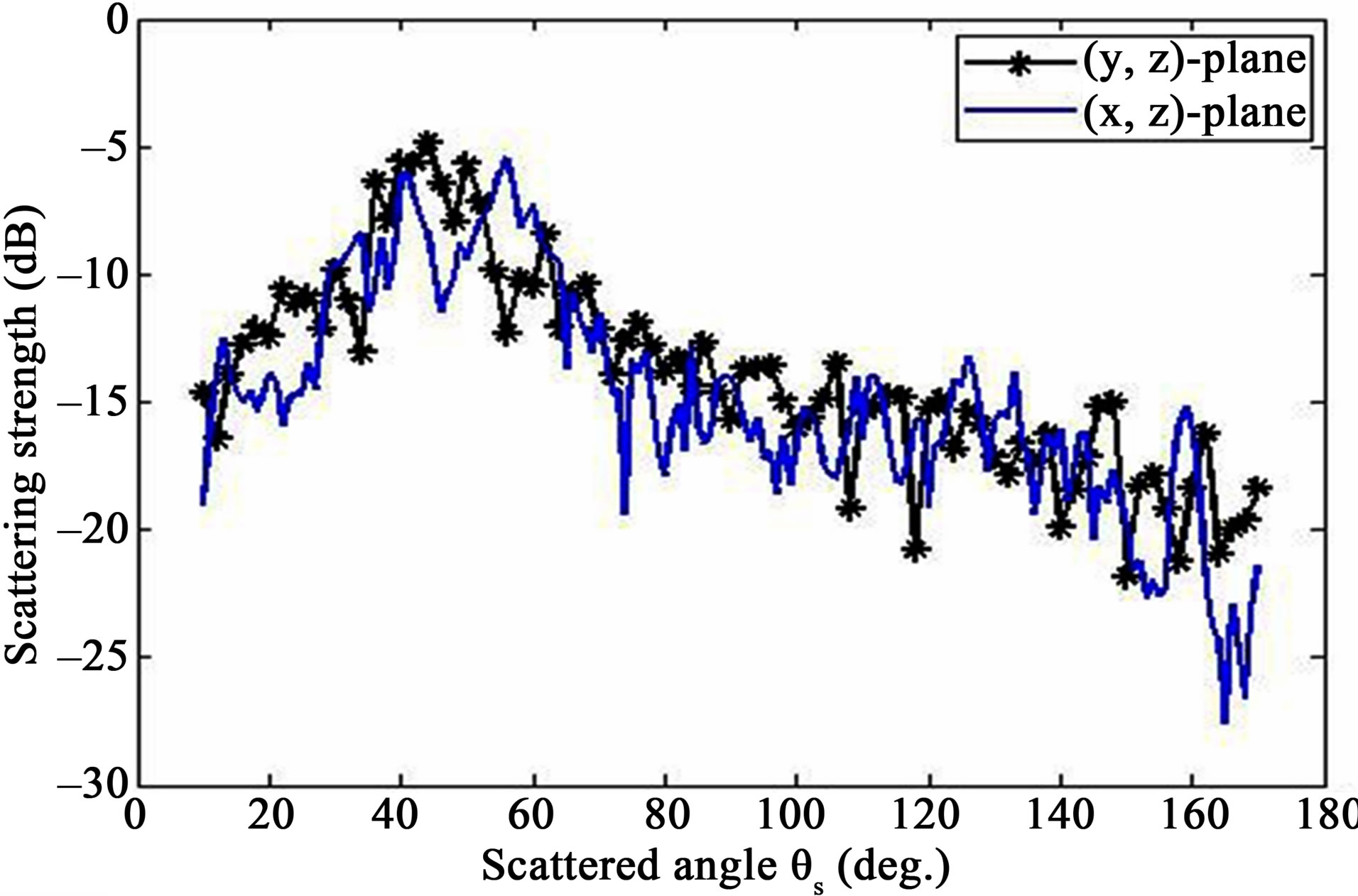
Figure 8. Plate 1, scattering strength as a function of the grazing scattered angle  for
for , median of 6 measurements per angle; (blue full line) propagation plane in the (x, z)-plane; (black full line with stars) propagation plane in the (y, z)-plane.
further than an angular band around the specular direction. The scattering strength predicted in the (x, z)-plane is mainly of the same order than the ones in the (y, z)- plane, the same dynamic is obtained for measurements from one plane to the other one.
In Figure 9, the maximum value is found around , which is the specular direction in this test case. The scattering strength predicted in the (x, z)-plane are mainly of the same order than the ones in the (y, z)- plane.
3.3. Measured Results: From an Anisotropic Surface (Plate 2 and Plate 3)
Figures 10 and 11 show the scattering strength as a function of scattered angle  in case of the anisotropic surface, Plate 2. The scattering strength data are obtained for
  in Figure 10 and for
  in Figure 11. For both angular configurations the data are measured such as the emitter and the receiver are in a plane, either the (x, z)-plane or the (y, z)-plane as it is described in Figure 2.
In Figure 10, there is an evident difference between the dynamic in the (y, z)-plane and the one in the (x, z)- plane. In the (y, z)-plane, the maximum value is clearly obtained in the specular direction for . An angular lobe of about 25˚ surrounding the specular direction is observed with a minimum value of about –15 dB. Then, for scattered angles in the band [10˚, 35˚] and [60˚, 170˚], the scattering strength is mainly equal or lower than –15 dB with a minimum value below –20 dB. In the (x, z)- plane, the scattering strength in the specular direction is not preponderant. The scattering strength varies a lot, and goes down to a value around –15 dB for scattered angles in the band [120˚, 170˚]. The maximum value around –5 dB is obtained for different scattered angles in the band
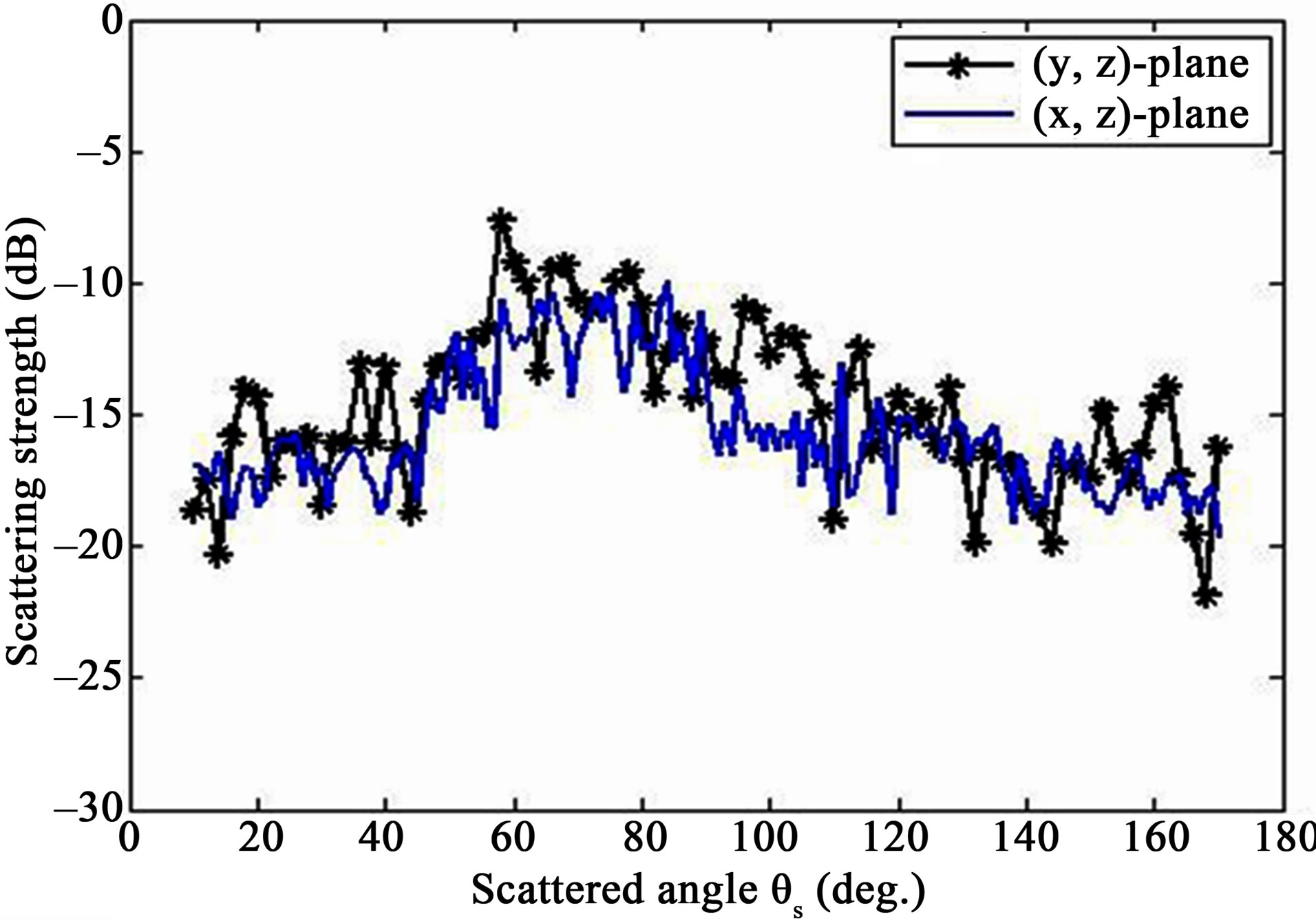
Figure 9. Plate 1, scattering strength as a function of grazing scattered angle  for
for , median of 6 measurements per angle; (blue full line) propagation plane in the (x, z)-plane; (black full line with stars) propagation plane in the (y, z)-plane.
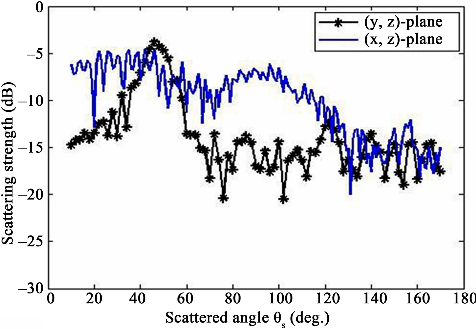
Figure 10. Plate 2, scattering strength as a function of grazing scattered angle  for
for , median of ten measurements per scattered angle; (blue full line) propagation plane in the (x, z)-plane; (black full line with stars) propagation plane in the (y, z)-plane.
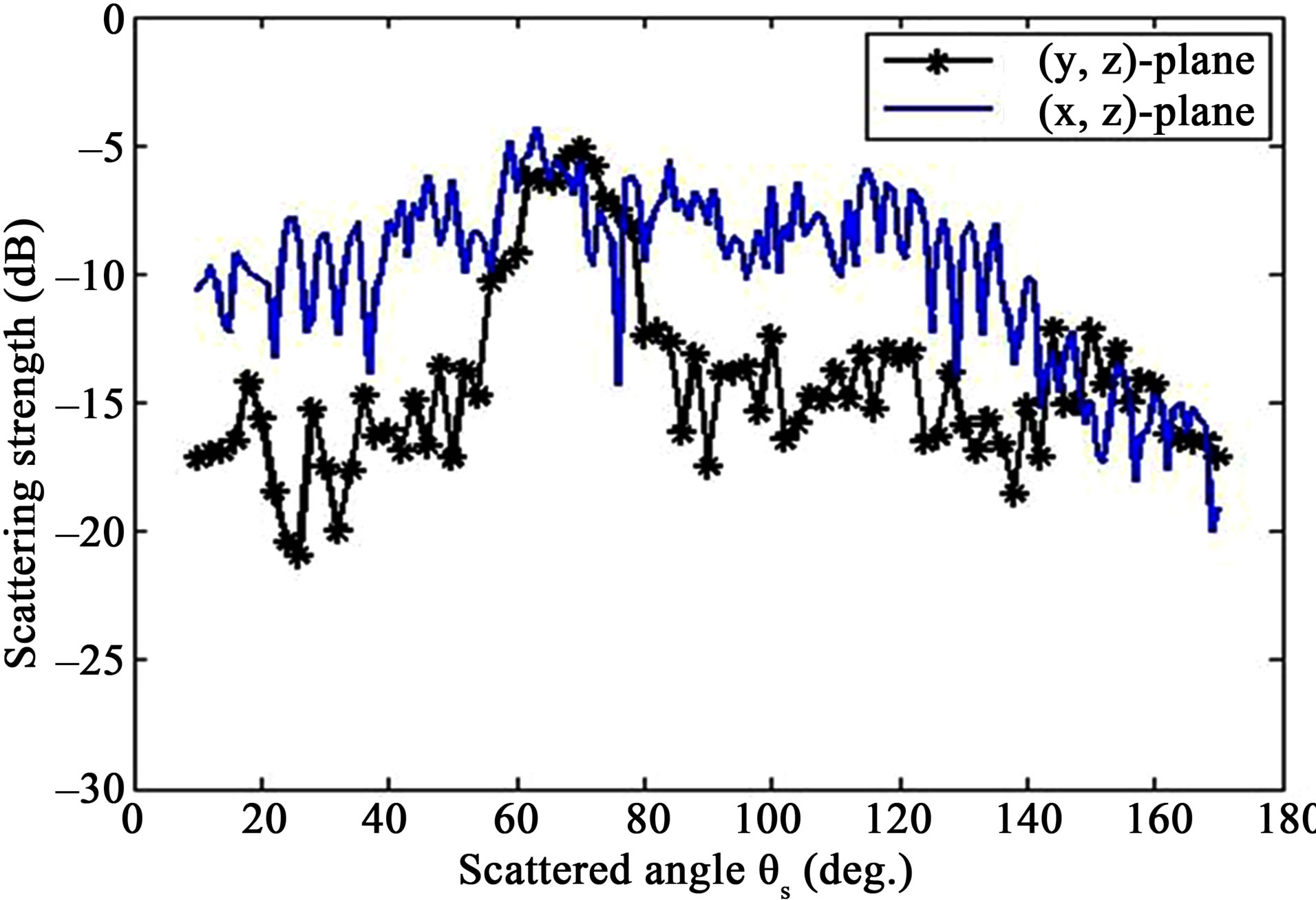
Figure 11. Plate 2, scattering strength as a function of grazing scattered angle  for
for , median of ten measurements per scattered angle; (blue full line) propagation plane in the (x, z)-plane; (black full line with stars) propagation plane in the (y, z)-plane.
[10˚, 50˚] and then a second maximum value around –7 dB is obtained many times in the band [50˚, 110˚]. There are many maxima and minima of importance in this propagation plane.
Figure 11 shows an apparent difference between the dynamic in the (y, z)-plane and the one in the (x, z)-plane too. In the (y, z)-plane, the maximum value of –5 dB is clearly obtained in the specular direction for . Then the scattering strength goes down to –15 dB, first at scattered angles equal to 50˚ and 85˚. Below
  and above
 , the scattering strength varies with values equal or lower than –15 dB. In the (x, z)-plane, the scattering strength in the specular direction is not preponderant as in the other propagation plane. The scattering strength varies between –15 dB and –5 dB for the scattered angle band [10˚, 130˚]. For a scattered angle higher than 120˚, the scattering strength varies with strong variations going mainly down.
Figures 12 and 13 show the measured scattering strength as a function of scattered angle  in case of the anisotropic surface, Plate 3. Similarly to the measured data obtained with Plate 2, there is a significant difference between scattering strength from the (x, z)-plane and the ones from the (y, z)-plane.
In Figure 12, the scattering strength obtained in the (y, z)-plane shows a maximum value about –7 dB in the specular direction, thus for . For a scattered angle lower and higher than the incident angle, the level decreases, going down to minimum values around –30 dB, particularly in the backward direction (
 ). In the (x, z)-plane, the specular direction does not show the maxi-
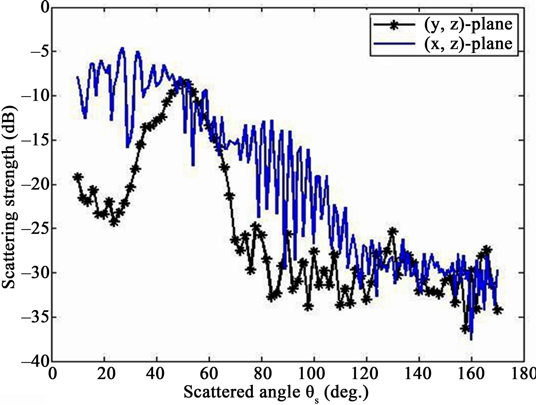
Figure 12. Plate 3, scattering strength as a function of grazing scattered angle  for
for , median of 5 measurements per scattered angle; (blue full line) propagation plane in the (x, z)-plane; (black full line with stars) propagation plane in the (y, z)-plane.

Figure 13. Plate 3, scattering strength as a function of grazing scattered angle  for
for , median of 5 measurements per scattered angle; (blue full line) propagation plane in the (x, z)-plane; (black full line with stars) propagation plane in the (y, z)-plane.
mum value of the scattering strength. The scattering strength fluctuates a lot from one maximum to a minimum, sometimes with 20 dB differences (around ). The maximum values are about –7 dB for scattered angles in the forward directions (
 ) and goes down in changing a lot to end around –30 dB in the backward direction
 . From
  to
to , scattering strength has got the same dynamic into the two different propagation planes.
Figure 13 shows, as well as the previous test case, a difference between the dynamic in the (y, z)-plane and the one in the (x, z)-plane. In the (y, z)-plane, the maximum value of –12 dB is clearly obtained in the specular direction for . The scattering strength goes down to –30 dB and varies around this value for scattered angle
  and
and . The scattering strength is higher mainly in the forward direction around the specular direction and is much lower in the backward direction as well as at shallow grazing angles. In the (x, z)-plane, the scattering strength in higher and fluctuates a lot around –15 dB for scattered angles between 10˚ and 100˚. For
 , the scattering strength still varies a lot but its mean value decreases to about –30 dB. For
 , scattering strength is globally similar to the one measured in the other propagation plane, the (y, z)-plane.
4. Summary and Discussion
The objective of this study was to evaluate the effects of particular rough surfaces through the bistatic scattering strength obtained in a water tank and to study the validity of the small slope approximation of first order used with particular structure function. Tank experiments have been set up to validate theoretical results obtained by testing the first small slope approximation with the structure function of different rough surfaces. the experimental validation has focused on three different plates. Plate 1 had been made based on a Gaussian distribution and particularly with the isotropic feature. Plate 2 and Plate 3 were based on a modified sine function, thus anisotropic and periodic. Notice that Plate 1 and Plate 2 have been built following a particular process. First the rough surfaces have been computed based on an analytical height covariance depending on the given parameters of each one. Once the height variations known, a sample surface has been made for each plate, then each one has been mould to finally get the plate in concrete. Due to this “homemade” process, Plate 1 and Plate 2 were heterogeneous (air bubbles into concrete) and also show a small roughness (size of order of a fine grain size), in addition to the roughness of interest, due to the sand used to make concrete. Plate 3 has been manufactured, was made of wax and was perfectly homogeneous.
For the simulations, the statistics of a Gaussian distributed surface were obtained straightforwardly using a structure function. For considering the statistics of Plate 2 and Plate 3, it was a bit more complicated in a sense that the structure function was obtained considering at the beginning a surface which is statistically based on a random stationary process. Assuming this rule, the structure function depended on a function taking into account the sine shape feature but also a random distribution of the height. Due to the differences between the theoretical rough surfaces and the rough surfaces used in practice, differences have been found between both predicted scattering strength and measured scattering strength (amplitude, angular lag between peaks, and so on).
Furthermore, one should notice that in theory the rough surface was assumed to be infinite. Contrary to the experimental data, the effect of the transducers, its directivity and the insonified area were not simulated when predicting the scattering strength. Thus, in case of Plate 2 and Plate 3, only few periodicities (and not an infinite number) are taken into account in the experimental scattering process, this may be one of the reasons why differences between predicted scattering strength and measured scattering strength have been found. Due to the differences between the theoretical set-up and the experimental one, the comparisons were based on the dynamic, the shape, and so on, of the scattering strength, but not on its absolute amplitude. Nevertheless, similar conclusions have been obtained between predictions and measured data and show the effect of particular rough surfaces (isotropic and anisotropic) on the scattering strength distribution.
For both simulations and experiments, scattering strength were analyzed as a function of grazing scattered angles for a particular grazing incident angle and an incident wave which frequency was 500 kHz, thus a 3 mmwavelength. The source and the receiver were in a same propagation plane, either in the (x, z)-plane or in the (y, z)- plane. For a periodic surface, the (x, z)-plane fit with the transversal direction of the sine relief (very rough), whereas the (y, z)-plane fit with its longitudinal direction (very smooth). All experimental data were obtained many times (minimum of 6 times and maximum of 10 times) with the same configuration and showed very similar results for each repeated test case with a maximum standard error of 0.1 dB.
Analysing theoretical and experimental results lead to the following conclusions. First, for an isotropic surface, the scattering strength is similar in one propagation plane compared to the other propagation plane, the (x, z)-plane versus the (y, z)-plane. The scattered energy is mostly distributed in the specular direction. Due to the fact that the scattering strength distribution is similar from one plane to another, it would possible in theory to simplify the scattering model. Instead of being based on a two dimensional surface, the structure function could be based on one-dimensional surface, that is a gain for simplifying the model and its calculation time. Then, for an anisotropic rough surface, the behavior is completely different from the analysis in the (x, z)-plane and the ones in the (y, z)-plane. In the longitudinal direction of the sine surface, the scattered energy is mainly distributed in the specular direction. Compared to the acoustic wavelength, the effect of the relief on the scattering phenomena is similar to the effect of a very smooth surface. On the contrary, in the (x, z)-plane, thus in the transversal direction of the sine relief, the scattering dynamic is totally different and tends to fluctuate a lot. The specular direction is not the principal direction for the scattered strength distribution anymore. Maximum values of scattering strength appear at different scattered angles, as well as many minimum values. The scattering strength varies a lot as a function of the scattered angle. This is probably due to the effect of the sine shape which is perfectly periodic for the experiment and partially periodic in theory. Nevertheless the scattering strength distribution may be related to the ratio between the acoustic wavelength and the dimensions of the relief, which are of the same order for the height and a bit larger for the surface wavelength.
On the one hand, the distribution of the scattered energy from an anisotropic surface showed that predictions via a model must take into account the entire two-dimensional surface in order to be sure of estimating all parameters which have an effect on the scattering strength distribution. On the other hand, the difference between propagation planes is a relevant piece of information, particularly for estimating the roughness from scattering strength data obtained from bistatic measurements and depending on the positions on the source and receiver. It would be worth also to analyse the scattering strength from an anisotropic surface as a function of several receivers whose position is not in the same propagation plane as the emitter. It would be of interest in order to find the most appropriate configurations where scattering data are the most useful, e.g. for estimating the roughness from scattering strength.
5. Acknowledgements
The authors would like to acknowledge the contributions of R. Guillermin for her assistance for the experiments at the Laboratoire de Mécanique et d’Acoustique (Marseille, France), M. Jaffrès and P.Martinat of ENSTA Bretagne (Brest, France) for providing the original anisotropic plate, B. Jaouen of IUP Génie Mécanique et Productique (Brest, France) for providing the original isotropic plate.
REFERENCES
- J. T. Anderson, D. Van Holliday, R. Kloser, D. G. Reid and Y. Simard, “Acoustic seabed classification: current practice and future directions,” ICES Journal of Marine Science, Vol. 65, No. 6, 2008, pp. 1004-1011. doi:10.1093/icesjms/fsn061
- A. J. Kenny, I. Cato, M. Desprez, G. Fader, R. T. E. Schüttenhelm and J. Side, “An overview of seabed-mapping technologies in the context of marine habitat classification,” ICES Journal of Marine Science, Vol. 60, No. 2, 2003, pp. 411-418. doi:10.1016/S1054-3139(03)00006-7
- K. Siemes, M. Snellen, D. G. Simons, J.-P. Hermand, M. Meyer and J.-C. Le Gac, “High frequency multibeam echosounder classification for rapid assessment,” Acoustics’ 08, Paris, 29 June-4 July 2008, pp. 4259-4264.
- L. Hellequin, J.-M. Boucher and X. Lurton, “Processing of high-frequency multibeam echo sounder data for seafloor characterization,” IEEE Journal of Oceanic Engineering, Vol. 28, No. 1, 2003, pp. 78-89. doi:10.1109/JOE.2002.808205
- C. Eckart, “The scattering of sound from the sea surface,” Journal of the Acoustical Society of America, Vol. 25, No. 3, 1953, pp. 566-570. doi:10.1121/1.1907123
- E. I. Thorsos, “The validity of Kirchhoff approximation for rough surface scattering using a Gaussian roughness spectrum,” Journal of the Acoustical Society of America, Vol. 83, No. 1, 1988,pp. 78-92. doi:10.1121/1.39618.
- F. G. Bass and I. M. Fuks, “Wave scattering from statistically rough surfaces,” Pergamon Press, New York, 1979.
- E. I. Thorsos and D. R. Jackson, “The validity of perturbation approximation for rough surface scattering using a Gaussian roughness spectrum,” Journal of the Acoustical Society of America, Vol. 86, No. 1, 1989, pp. 261-277. doi:10.1121/1.398342
- D. R. Jackson, D. P. Winebrenner and A. Ishimaru, “Application of the composite roughness model to high-frequency bottom backscattering,” Journal of the Acoustical Society of America, Vol. 79, No. 5, 1986, pp. 1410-1422. doi:10.1121/1.393669
- D. R. Jackson, “APL-UW high-frequency ocean environmental acoustic model handbook,” Technical report, Seattle, 1994.
- K. W. Williams and D. R. Jackson, “Bistatic bottom scattering: model, experiments, and model/data comparison,” Journal of the Acoustical Society of America, Vol. 103, No. 1, 1998, pp. 169-181. doi:10.1121/1.421109
- D. R. Jackson and M. D. Richardson, “High Frequency Seafloor Acoustics, the Underwater Acoustics Series,” Springer, New York, 2007.
- J. W. Choi, J. Na and W. Seong, “240-kHz bistatic bottom scattering measurements in shallow water,” IEEE Journal of Oceanic Engineering, Vol. 26, No. 1, 2001, pp. 54-62. doi:10.1109/48.917926
- J. W. Choi, J. Na and K.-S. Yoon, “High-frequency bistatic seafloor scattering from sandy ripple bottom,” IEEE Journal of Oceanic Engineering, Vol. 28, No. 4, 2008, pp. 711-719. doi:10.1109/JOE.2003.819151
- A. G. Voronovich, “Wave scattering from rough surfaces,” Springer, New York, 1999.
- T. M. Elfouhaily and C.-A. Guerin, “A critical survey of approximate scattering theories from random rough surfaces,” Wave Random Complex Media, Vol. 14, No. 4, 2004, pp. 1-40. doi:10.1088/0959-7174/14/4/R01
- E. I. Thorsos and S. L. Broschat, “An investigation of the small slope approximation for scattering from rough surfaces. Part I. Theories,” Journal of the Acoustical Society of America, Vol. 97, No. 4, 1995, pp. 2082-2092. doi:10.1121/1.412001
- S. L. Broschat and E. I. Thorsos, “An investigation of the small slope approximation for scattering from rough surfaces. Part II. Numerical studies,” Journal of the Acoustical Society of America, Vol. 101, No. 5, 1996, pp. 2615- 2625. doi:10.1121/1.418502
- R. F. Gragg, D. Wurmser and R. C. Gauss, “Small slope scattering from rough elastic ocean floors: general theories and computational algorithm,” Journal of the Acoustical Society of America, Vol. 110, No. 6, 2001, pp. 2878-2901. doi:10.1121/1.1412444
- S. L. Broschat and E. I. Thorsos, “An investigation of the small slope approximation for scattering from rough surfaces. Part II. Numerical studies,” Journal of the Acoustical Society of America, Vol. 101, No. 5, 1996, pp. 2615- 2625. doi:10.1121/1.418502
- A. P. Lyons, W. L. J. Fox, T. Hasiotis and E. Pouliquen, “Characterization of the two-diemensional roughness of wave-rippled sea floors using digital photogrammetry,” IEEE Journal of Oceanic Engineering, vol. 27, No. 3, 2002, pp. 515-524. doi:10.1109/JOE.2002.1040935
- J. E. Moe and D. R. Jackson, “First-order perturbation solution for rough surface scattering cross section including the effects of gradients,” Journal of the Acoustical Society of America, Vol. 96, No. 3, 1994, pp. 1748-1754. doi:10.1121/1.410253
- D. R. Jackson, “High-frequency bistatic scattering model for elastic seafloors, technical memorandum,” Technical report, Seattle, 2000.