Journal of Mathematical Finance
Vol.06 No.05(2016), Article ID:72056,23 pages
10.4236/jmf.2016.65052
Pricing the Credit-Risk Put Embedded in Borrowers’ Extendible Credit Commitments, with Its Application to Basel-3 Micro-Prudential Regulation
John-Peter D. Chateau
Faculty of Business Administration, University of Macau, Macau, China

Copyright © 2016 by author and Scientific Research Publishing Inc.
This work is licensed under the Creative Commons Attribution International License (CC BY 4.0).
http://creativecommons.org/licenses/by/4.0/


Received: July 15, 2016; Accepted: November 14, 2016; Published: November 17, 2016
ABSTRACT
This research makes two contributions: 1) use a term structure framework to price analytically the put option implicit in borrowers’ extendible credit commitments and 2) use the latter to compute in a ratings-based model the capital charge corresponding to the credit-risk exposure of such commitments. Since the term structure of interest rates is stochastic, the zero-coupon bonds in the put closed-form solution delink discounting factor from the credit and funding rates that define the credit spread appearing in the put payoff. By essence, extendible commitments straddle the term- based commitment classification of Basel-3 simplified approach. To improve this, we formulate a ratings-based model that combines extendible put values with new coefficients (forward funding proportion and exposure at funding) as well as a matrix that captures credit-ratings migration over time. Moreover, the combination is versatile enough to deal with a borrower’s credit downgrade and its attendant incremental Basel-3 capital charge.
Keywords:
Extendible Put and Extension Premium Embedded in Once-Extendible Commitments, Capital Charge for the Credit-Risk Exposure of Extendible Commitments, Cost of Borrower’s Rating Downgrade Based on a Credit-Rating Migration Matrix

1. Introduction
This paper offers a solution to the following problem: How to account for the credit- risk exposure of extendible loan commitments subject to Basel-3 micro-prudential regulation. There are two steps to the solution: Derive first in a term structure framework the put value embedded in borrowers’ extendible credit commitments and use it next in a ratings-based model to compute the capital charge corresponding to the credit-risk exposure of once-extendible commitments.
Longstaff [1] was the first to derive analytical solutions for extendible options, and more specifically for the holder-extendible put option examined here. As reported in Shevchenko ( [2] , under Equation (32)), there are several typographical errors in Long- staff’s Equation (12) for the holder-extendible put (some being also repeated in Haug [3] ). To the best of our knowledge, the first mathematically correct expression for the holder’s (here the borrower’s) once-extendible put option is to be found in Wu [4] ; subsequently a more general treatment of single-period extendible puts is given by Shevchenko [2] and the general closed-form solution for n-time extendible options is provided by Chung and Johnson [5] . Gukhal [6] provides valuation of extendible op- tions under the jump-diffusion process and Peng and Peng [7] under the more restric- tive jump-fractional Brownian process. Extendible options find applications in several fields of finance: let us mention but a few. They are applied to real estate by Longstaff [1] , warrants by Hauser and Lauterbach [8] , bonds by Athanassakos, Carayannopoulos and Tian [9] and Longstaff ( [1] , Section 4), corporate finance by Wu, Yu and Nguyen [10] and Wu and Yu [11] , and petroleum concessions by Dias and Rocha [12] . Ibrahim, O’Hara and Constantinou [13] apply the fast Fourier transform to improve their computational efficiency when the once-extendible options are derived as semi-analytic expressions. Regarding their application to credit commitments more specifically, we found but one reference, Chateau and Wu [14] . Yet in their borrower’s extendible expression, Equation (9)1, discounting is done over two different periods with a constant risk-free rate of interest. Yet keeping a constant discounting rate becomes problematic when simultaneously stochastic credit and funding rates are defining the credit spread2 that appears in the put payoff. To solve the problem, we derive a put expression that re- lies on a stochastic term structure of interest rates (hereafter referred to as stochastic Tsir). Here the latter is formalized by one factor, the short-term riskless rate of interest; and all rates (credit, funding and discounting ones) are stochastic with discounting done with zero coupon bonds (ZCBS). The Feynman-Kac theorem and a change of nu- meraire enable us to delink discounting factor and spread rates appearing in the put payoff. This approach leads to pricing the extendible put and its extension premium under forward risk neutrality at the extension date.
Since Thakor, Hong and Greenbaum [15] , the credit or spread risk of loan commit- ments is apprehended by an embedded put option that is used to compute the Risk- Weighted Amount (RWA) of commitments and their capital charge mandated by Basel-3 micro-prudential regulation―see Basel Committee on Banking Supervision [16] and [17] . According to Basel-3 standardized simplified approach, the initial term of commitments (less than or longer than one year) determines the way credit-conver- sion and principal-risk coefficients as well as RWAS of irrevocable commitments are computed. Yet, our reference scenario, namely a one-year commitment extendible for another one, straddles this Basel time divide and thus challenges this term-based granularity. For instance, should our one-year commitment extendible for another one be classified as less or longer than one year? It is obviously less than one year if it is exercised in the initial period or if the borrower does not choose to extend beyond the initial period, but it is indeed longer than one year if exercised at or after the extension date or not at all at the end of two years. Since extendible commitments are term-wise hybrid instruments, we propose to replace Basel simplified approach by an Advanced Internal-Ratings Based (AIRB) model that allows credit risk to be spread over at least two time periods. The capital charge regarding the credit-risk exposure of extendible commitments is computed by combining the embedded put value with two new coefficients. The first one is a forward funding proportion (namely the credit line take-down proportion relevant for the commitment extension period) and the other one is the exposure at funding (practically the first coefficient applied to the bank’s aggregate amount of still unused loan commitments). In extendible commitments moreover, banks also have to assess the borrower’s creditworthiness over multiple periods. To wit, assume that a prime-rate borrower of a once-extendible commitment is initially benchmarked as a triple-A credit rating; yet at the extension date, the bank will extend the commitment under the initial conditions only if the borrower maintains this triple-A rating. If it is not the case, any rating downgrade relies on transition probabilities that capture the credit-ratings migration over time. The mapping of indebtedness values (namely the marked-to-market value of line commitments) into credit-risk ratings allows banks to determine the incremental credit-risk capital charge caused by a rating downgrade of any fraction of their extendible commitments. In addition, the ratings-based model is versatile enough to deal with downgraded borrowers who may face higher spreads.
The layout of the paper is as follows. Beyond a short review of how Basel-3 apprehends commitment credit risk, Section 2 introduces the analysis-relevant features spe- cific to extendible commitments as well as the indebtedness forward value and its log- returns. Next the closed-form expression of the European forward put option embedded in once-extendible commitments is derived and the transition probabilities of credit-ratings migration over time are formalized. Section 3 explains simulation pa- rameters and estimate meaning before highlighting two significant patterns emerging from the estimates of extendible put values and extension premiums. In Section 4 the previous simulations are used in an AIRB model to compute the capital charge for extendible commitments as well as the incremental cost implied by a borrower’s credit downgrade. Short concluding remarks close the paper in Section 5.
2. The European Put Option Embedded in a Once-Extendible Credit Commitment
2.1. How Commitment Credit Risk Is Apprehended under Basel-3
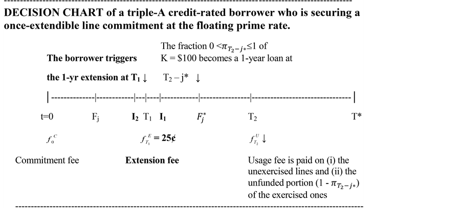
Since Thakor, Hong and Green baum [15] , the credit risk of loan commitments is ap- prehended by an embedded put option that oftentimes is used to compute the risk- weighted amount of commitments subject to Basel-3 capital requirements (see Basel Committee on Banking Supervision, [16] and [17] ). Before examining extendible com- mitments specifically, three Basel-3 relevant commitment features have to be briefly re- viewed: the origin of the implicit put option, when and why it is European, and how to endogenize any credit line draw-down3. They are integrated in the decision chart below.
A floating prime-rate credit commitment allows a borrower to draw, say, over a one-year period [0, T1] up to K = $100 at a floating prime rate , namely a date-0 fixed markup plus a date-j stochastic cost of funds, j being the date at which funding takes place, with 0 ≤ j ≤ T1. The funding risk
  being borne by the borrower, the lat- ter is not relevant for computing the bank’s capital charge for commitment credit risk under Basel-34. It is the fixed markup
  that generates the embedded put option, for any prime-rate borrower can secure date-0 funding either through a credit-line com- mitment or a demand loan characterized by a stochastic spot markup m0 = l0 ? c0―(l0) denoting the spot floating prime rate and c0 the bank’s funding rate in the banker’s ac- ceptances market (the rate on certificates of deposit is also used as exogenous index). Fixed and variable markups enable us to define the j-month-old indebtedness forward5 value Fj as:
 with
with , (1)
, (1)
where  is the difference between the date-0 fixed markup and the date-j spot markup, (T* ? T1) is loan duration (say one year) once the commitment has been exercised and K is the constant line par value. In the decision chart for instance, for an initially one-year commitment starting July 1st and running to June 31st, F6 denotes a six-month-old indebtedness value (j = 6) which still has a remaining six-month term to maturity (T1 ? j). The monthly log returns of an indebtedness forward value that is con- tinuously j-month old are given by
 (2)
(2)
where σ denotes the volatility of the indebtedness forward value and W the Wiener process.
At any date j, fluctuations in the variable markup of spot loans result in either  or
or . In the first case, the rational commitment holder decides to draw on the line because the latter fixed markup is less than the stochastic spot markup. This then gives rise to an implicit put option as the borrower’s debt value Fj is less than the option strike price K. On the other hand, when
  the rational borrower chooses a spot loan instead of drawing on the credit line; there then is no embedded credit-risk put. In short, spot markup fluctuations at valuation date j give rise to a j-month put option embedded in an initially one-year line commitment.
At yearend, usually the date of the bank’s audit under Basel-3 regulation, j-month old commitments have various remaining time to expiry. By making date j the option valuation date and by assuming for clarity that it coincides with Basel yearend audit date, the time remaining to commitment expiry then becomes the remaining life of contract―as in Merton [25] . For instance our one-year (July to June) commitment is 6-month old at the end of December when the Basel audit takes place, so generating a 6-month put option. It is thus the Basel framework that makes the put option Euro- pean6. Finally, when the commitment is j-month old, the borrower can still draw on the credit-line unused portion over the forward period T1 ? j. The magnitude of this line draw-down  is a function of the time remaining to commitment maturity: the longer this forward period, the greater is the borrower’s potentialline draw-down7.
In short, indebtedness value and credit-line remaining term to maturity are the two most important determinants in valuing the implicit commitment put. Granted these features, the European put option on indebtedness forward values is usually priced as a Black [27] one-period European forward put option8: namely
 , (3)
, (3)
where , and
, and .
.
In Equation (3),  denotes the date-0 zero coupon bond that pays $1 at T1, N[\] the standard univariate cumulative normal distribution function, d1 the standard moneyness with
  and σ the volatility of the indebtedness forward value. A ZCB discount factor is chosen for consistency with the stochastic Tsir and for- ward-risk neutral valuation of the extendible put option introduced in Subsection 2.3.
2.2. Features Specific to Borrowers’ Extendible Credit Commitments
The decision chart also captures the salient features of our reference scenario, the one- period commitment extendible for another one: the purpose is to value the embedded extendible put within Basel time frame, and thus not to value the various components of loan commitments9. In the chart, the bank originates at date 0 a commitment with the following features: (1) the initial one-year commitment period, [0, T1], is extended at T1 for a single one-year period, [T1, T2], at the borrower’s option, (2) loan duration, [T2, T*], is one year from date T2 if the credit line (CL) is drawn down, (3) the latter face value remains constant over both commitment and extension periods (namely K1 = K2 = $100), and (4) the floating prime-rate formula is . As explained in the previous subsection, only the date-0 fixed forward markup
  is relevant for Basel-3 commitment credit-risk analysis. And it remains constant over the two one-year peri- ods, say at 1.5% per annum, under the following condition: the extension is granted only if the date-0 triple-A rated prime borrower remains so at date T1.
Thakor and Udell [29] 10 provide the economic rationale for the bank’s optimal deployment of up-front and rear-end fees in non-extendible commitments. When their sorting variables are adapted to the borrower-extendible commitment, fees (here stan- dardized for argument sake at 1/4 of 1% per annum of the line maximum face value, namely 25 cents per $100) are deployed at origination (t = 0), extension (T1) and end (T2) dates in the decision chart. The first fee is the upfront commitment fee , the second one is an extension fee,
  cents, and the third one is a rearend or so- called usage fee,
  (The latter may or may not be paid at T2 on the un-drawn por- tion of the credit line). Only the extension fee is of relevance for pricing the put implicit in extendible commitments. We are now in a position to state how the decision se- quence runs. The borrower does not draw down the CL in the initial commitment pe- riod but then triggers the extension at date T1 upon paying the extension fee
  with two possible outcomes up to date T2. From date T1 and up to date T2, the CL is either exercised and partial or total funding of the $100 results in an on-balance-sheet loan, or alternatively the commitment simply expires at T2 with the borrower paying the rear- end fee on the unexercised lines. He also pays the latter on the un-funded portion of the exercised lines. To be complete, notice that the one-year non-extendible commitment is but a special case nested in the extendible-commitment model. In that case, the bor- rower draws on the line at any date up to date T1, with the one-year corporate loan, [T1, T*], becoming outstanding immediately.
At this juncture, it is already worth indicating that three of the decision-chart as- sumptions will be relaxed in subsequent developments. There are: (1) the extension pe- riod can be lengthened to two or more years, (2) the prime markup that captures credit risk can be adjusted by add-ons or discounts (±25 basis points, ±50 basis points, and so on) for non-prime commitments11, and (3) higher credit spreads of non-prime com- mitments are associated with lower credit ratings of external rating agencies (more on this in Subsection 2.4). Finally, the parameters I1 and I2 defining the extension interval are introduced in the upcoming subsection.
2.3. Valuing the Borrower’s Put Embedded in a Once-Extendible Credit Commitment
We denote the European extendible put payoff as
 , (4)
, (4)
where K1 and K2 are the line par value at dates T1 and T2 respectively,  is the in- debtedness forward value at date T1 and
  the date-T1 extension fee. We label g(T1) and g(T2) the payoff components with date T1 and date T2 respectively, and now deal with them in turn.
According to the Feynman-Kac theorem, the date-0 extendible put value is written as
 , (5)
, (5)
where E* denotes expectation taken with respect to the probability distribution implied by the risk neutral process
 ,
,
where μ*(.) and s(.) are the drift and volatility of the process and dW(t) its Wiener dif- ferential. To delink discount factor and payoff in Equation (5), namely to eliminate the
covariance between discount factor and payoff,  , we use a change
of numeraire12 such that
 ,
,
where  denotes a ZCB that pays off $1 at time T1. Underlying the ZCB is the one-factor risk-neutral Tsir characterized by the stochastic short-term interest rate, r. This implies using the date-T1 forward risk-neutral bond price process and short rate process

 ,
,
where µz and σz are the drift and volatility of the ZCB. The drift of drt has been adjusted for the forward expectation operator. We can now write that
 , (6)
, (6)
where  denotes expectation under forward risk neutrality. Equation (5) is then re- written
 . (7)
. (7)
Equation (7) has the advantage to delink the discount factor from the credit-risk spread embedded in , the indebtedness value appearing in the put payoff g(T1). Repeating the same procedure (Feynman-Kac, change of numeraire and forward risk- neutrality) for the g(T2) component with a date-T2 payoff yields13
 . (8)
. (8)
At extension date T1, the borrower can either (1) let the put expire worthless if , or (2) exercise the put and get
  if
if , or (3) pay
  to extend the put to T2 if
 . As shown in the decision chart, I1 denotes the higher bound of the extension region and I2 the lower one (I2 < K1 < I1 implies moving from out-of-the money to in-the-money)). Case (3) comprising the extension is now devel- oped as follows
 (9)
(9)
where . The values of the two bounds to the exten-
sion region in Equation (9) are found by solving two nonlinear equations, using for instance the Newton-Raphson algorithm coupled with a bisection algorithm when derivatives are close to zero. This means solving
 (10)
(10)
and
 (11)
(11)
Equation (10) has one solution but Equation (11) may have one solution or none since r = δ in forward or futures options. The derivation of the closed-form solution to Equation (9) is tedious but straightforward ? the solution is outlined in the Appendix. The value of the extension premium (EPi)14 (with i denoting the length of the extension period in years) is:
 (12)
(12)
In Equation (12) ρ, x, x*, z1 and z2 are defined as follows when t = 0:

 ,
, 
 ,
, 
In addition N[\] is the standard univariate cumulative normal distribution function, N2(\, \, −ρ)15 is the standard bivariate cumulative normal distribution function with correlation −ρ, and  the one-year Black’s forward put option at date 0 --the other terms having been defined previously. Adding the one-year straight put to Equation (12) yields the once-extendible put value, EVPi, with i denoting again the length of the extension period in years:
 (13)
(13)
Rearranging further Equation (12) provides a more intuitive interpretation based on the ZCBS generated by the Tsir:
 (14)
(14)
Equation (13) highlights the fact that Black one-year straight put as well as the next two terms are discounted with a one-period ZCB, while the last two ones are dis- counted with a two-period ZCB. The second term is a put having boundary I2 as strike (more precisely as strike in moneyness z2), the third is the probability-weighted (the square-bracket term in the third term of Equation (12)) discounted fee and the last two terms, the difference of two puts with boundaries I2 and I1 as strike values in their z2 and z1 moneyness respectively. As three put values depend on the I1 and I2 strike values in Equation (13), it is worth focusing on the two forces that impinge on the width of the extension interval:
1) When the duration of the extension period increases (say from one to five years as in the numerical illustration in Section 3 below), the extension interval [I2, I1] widens progressively about $100. This effect is apprehended by the term condition of Equation (10).
2) But when the bank increases the extension fee, the other parameters remaining constant, the extension interval [I2 < I1] first shrinks continuously up to being reduced to a point before reversing to [I2 > I1] --with the unattractive result of a negative exten- sion premium. For the once-extendible commitment, the extension premium shrinks to 0 when  increases to $1.499855; and when the bank raises the fee beyond this value, the borrower’s extension premium turns negative. Yet the borrower has to weight the fee paid to the bank against the benefit expected from the extension, namely the extension premium. The impact of the magnitude of the extension fee on the bounds of the extension interval is apprehended by Equation (11), which may have one solution or none.
Finally, it remains to determine how the ZCB values are computed in Equation (12). The easiest way is to use the actual market values of the Canadian ZCBS, with the Tsir estimation computed daily by the Bank of Canada (see Bolder, Johnson and Metzler [34] ). The alternative to market values is to use the class of “normal” models of the in- terest rate, namely models such as Ho and Lee [35] , Vasicek [36] or Hull and White [37] . The latter based on the term structure of volatilities has the advantage to reconcile model and market values. In the numerical illustration a flat Tsir is used for the sake of simplicity.
2.4. Transition Probabilities between Commitment Credit Ratings
The value of the put just derived is conditional on the borrower continuously remain- ing a floating prime rate borrower with a triple-A credit rating. Yet, the borrower who is bank-classified as prime at the time of commitment writing may actually turn out to be less than prime over the life of the extendible commitment. Does a rating downgrade at the extension date leads to an incremental credit-risk charge, and if so, how is the latter computed? We propose to compute the latter in three steps: select relevant transi- tion probabilities between borrowers’ credit ratings, map declining risk ratings into progressively in-the-money (ITM) indebtedness values, and combine the transition probabilities with the values of the extendible put option derived in Subsection 2.3.
In the first step, borrowers’ downgrades should ideally be apprehended by transition probabilities specific to commitment credit ratings. Yet presently, since Basel-3 com- mitment granularity is term-based instead of credit-ratings-based, this type of informa- tion is not publicly available. So by default, we fall back on a credit-migration matrix based on corporate bonds. More specifically, we choose the one-year transition prob- abilities from the model of Xing, Sun and Chen [38] , which are based on Markov chains with stochastic structural changes in the credit-rating probability transitions16. In Exhibit 1, only the transition probabilities between ratings of investment grade bonds are shown. This matrix assigns an S&P triple-A rating to a borrower who is bank-classified
Exhibit 1. Posterior means of the transition probabilities (in per cent) estimated from the model of Xing, Sun and Chen [38] : their Tableau 1 is based on Standard & Poor’s credit ratings for the period spanning October 2008 to September 2009. Probabilities reported here are only between investment-grade credit ratings.

as a floating prime-rate borrower at the time of commitment writing, with an 89.97% probability of remaining prime over a one-year commitment term. But suppose that at any time up to commitment extension, the bank concludes that it wrongly assessed the prime borrower’s credit worthiness, which happens to be one notch lower at double-A. The commitment being a binding contract, the borrower keeps her initial fixed markup , while she normally would be subject to a greater spread say prime plus a 50-basis-point add-on17. Then,
  bps implies in Equation (1) that Fj = $99.5 < K1 = $100. In other terms, a credit downgrade translates into a greater non-prime spread and hence a lower indebtedness forward value. This second step is formalized by the two rows above the matrix of Exhibit 1, where progressively ITM indebtedness values are mapped into declining credit-risk ratings18. In the third step, the transition matrix is twinned with the extendible put values computed in the next section.
3. Simulation Results of Extendible Put Values and Extension Premiums
3.1. Simulations and Estimate Meaning
As indebtedness values are non-traded banking assets, put values embedded in extendi- ble commitments are but notional values to be estimated by simulations based on the statistical evidence presented in Exhibit 2 below. To be consistent with our reference scenario (the one-year commitment extended for another one), the indebtedness val- ues are computed with a one-year markup differential ( ) between the commit- ment fixed spread and subsequent stochastic markup of spot loans. The min and max values in Exhibit 2 imply that the indebtedness value Fj ≡ F12 varies in the value range
Exhibit 2. Statistical analysis of ln[tFj/t−1Fj], the indebtedness-value monthly change relatives, computed from Equation (2) for the period 1988.01 to 2015.12 (n = 336 monthly observations). Date j is always 12 months after commitment origination.
Source: Spot markups and markup differentials used in computing Equations (1) and (2) are based on Statistics Canada monthly time series V122495 and V122504 of the prime credit rate and one-month banker’s acceptance of chartered (commercial) banks, respectively.
$96.52 to $103.23, with $100 being par value: we thus set Fj at $100, $99.5, $99, $98.5, $98 and 97.5, since under Basel-3 we are only interested in commitments puts that move progressively ITM19. Granted these indebtedness values, simulation experiments are performed for the one- and two-year non-extendible commitments  and
and  and several borrower-extendible commitments; for the latter ones, the initial commit- ment runs from date t = 0 up to T1 with one-to-five year extension periods starting at date T1. The following parameters are common to all simulations: the credit-line strike price remains constant through time, K1 = K2 = $100, the interest rate in the flat Tsir is r = 0.04, and r = (T1/T2)1/2. Since the volatility of the indebtedness-value change rela- tives reported in Exhibit 2 is low (s = 0.004329 or 1.499% on an annual basis), the simulations are performed with a 3% annualized volatility, namely s = 0.03.
Next, we clarify the meaning of the values computed for the reference scenario when the indebtedness value is slightly ITM at F = $99. Put values and extension premiums are shown in the entries in column (3) of the matrices of Table 1. According to the first boldfaced entry in column (3), the estimate  = $1.688 means that the European put embedded in a one-year straight commitment has an equilibrium value of 1.688% of the $100 par value if the floating prime-rate commitment with a 1.5%-p.a. fixed for- ward markup is priced when the stochastic markup on spot loans is 2.5% p.a. By way of contrast, when the original one-year commitment is extended for another year, the value of the extendible put, EPV1, shown in the cell corresponding to row (1a) and column (3) of matrix 1, is greater at $1.919. Put values of commitments with longer extensions are also computed, with EPV5 = $2.56 corresponding to a commitment with a five-year extension period. The magnitude of the extension premiums comprised in borrower-extendible commitments is shown in matrix 2. For our reference scenario in column (3) again, EP1 = $0.23, namely the extension premium amounts to only 12.1% of the one-year extendible put value; but when the extension duration increases to five years, EP5 = $0.874, namely it increases to 34.12% of the five-year extendible put value.
3.2. Risk-and-Term Patterns Emerging from Extendible Put Values and Extension Premiums
Two patterns of extendible put values are emerging from the matrices in Table 1; they are also visualized in Figure 1. The first pattern highlights the magnitude of the notional
Table 1. European put values (EPVi) and extension premiums (EPi) embedded in extendible credit commitments.
Valuation date is t = 0. Entries on row 1: Fj indebtedness forward values computed in Equation (1). Entries in row 2 and row 3:  and
and  the European put values implicit in one- and two-year straight commitments. Entries in matrix 1: extendible put values in dollars, EPVi, from Equation (13), with extension terms i: 1, ∙∙∙, 5 years. Entries in matrix 2: extension premiums, EPi from Equation (12), with i: 1, ∙∙∙, 5 years, in $ and in % of the corresponding extendible put values, respectively. Parameter definitions: Fj indebtedness forward value in $; K1 = K2: credit line exercise value in $; r = short rate characterizing the term structure of interest rates, in % per annum; σ = indebtedness- value volatility in % per annum; T1 and T2 initial and terminal commitment maturity dates. Common variable values: K1 = K2 = 100; r = 0.04; σ = 0.03; T1 − t = 1; T2 − T1 = 1, ∙∙∙, 5;
 .
.

Figure 1. $ Sensitivity of extendible put values (EPVi) and extension premiums (EPi) to (i) indebtedness forward values with corresponding credit-risk ratings and (ii) i-term extension.
liability incurred by the bank for carrying unused credit lines with varying extension terms. The rows and columns of matrix 1 show the put sensitivities to risk and term: credit-risk variations (namely indebtedness-value variations) are shown across rows while extension-term variations are shown down columns. Visual inspection of matrix 1 as well as the upper surface in Figure 1 reveal that put values, and hence commitment credit risks, increase (1) steadily when indebtedness values are moving progressively ITM, but (2) more slowly when extension periods are growing longer. To wit, in row (1a) for a commitment that offers a one-year extension, EPV1 increases from $1.396 for an at-the-money (ATM) indebtedness value to $2.889 for the deeper ITM indebtedness value of $97.5. The other rows depict similar put-like value curves. By way of contrast, the matrix columns capture the put sensitivity to extension terms. More concretely, for Fj = $97.5 in the last column, put values are increasing from $2.889 for a straight com- mitment to $3.369 for a commitment with a five-year extension period. In brief, matrix 1 of Table 1 and the upper surface of Figure 1 clearly indicate that extendible put val- ues and hence bank credit-risk costs are more sensitive to indebtedness-value risk variations than to extension-period duration.
The other pattern, revealed from the rows and columns of matrix 2, shows that the extension premiums expressed in $ terms or as a percentage of the EPVi-values are: (1) increasing with the length of the extension period (down any column), but (2) declin- ing when the indebtedness value moves deeper ITM (across each row). According to entries on row (a) of matrix 2 for instance, the one-year extension premium as a per- centage of EPV1 declines from 17.64% to 5.93% when the indebtedness values move deeper ITM. But from the other rows of matrix 2, the extension premiums implicit in longer-term extendible commitments are percentage wise much larger than those em- bedded in short-term commitments: they vary for instance from 45.61% to 19.33% for the five-year extension premium. Figure 1 highlights the dichotomy for $ values: when indebtedness values are moving ITM the extendible put upper surface is upward slop- ing whereas simultaneously the extension-premium lower surface is downward sloping. Yet both surfaces react positively but to different degrees to longer extension terms.
These simulation results are used in the next section to quantify Basel-3 risk- weighted capital charge for extendible commitments.
4. Application: A Basel-3 Ratings-Based Model of Extendible Loan Commitments
4.1. Basel-3 Commitment Framework
Beyond its macro-prudential reform, Basel-3 also targets bank-level or micro-prudential regulation (see Basel Committee on Banking Supervision [17] or Le Lesle and Avra- mova [45] ). Presently, according to Basel-3 standardized approach, the initial term of commitments determines the way the RWAS of irrevocable commitments are computed. Regarding those with an initial term less than one year, a 20% credit-conversion factor (CCF) is first applied to the commitment face value and next, a 100% principal- risk factor (PRF) is applied to this credit-equivalent amount. For longer-term irrevocable commitments, Basel-2 50% CCF and 100% PRF remain in force and, for all revocable commitments irrespective of their term-to-maturity, 0% CCF and PRF apply. Moreover and independently of initial term, Basel-3 does not distinguish between prime- and non-prime-rate commitments, nor does it take into account their credit ratings. By way of contrast, outstanding corporate loans are classified according to the credit ratings of external rating agencies, with maturity being only a secondary adjustment. The prob- lem is that, when an off-balance-sheet commitment is drawn upon, this amount be- comes an on-balance-sheet loan alongside the other spot loans, with the same coeffi- cients applying to draw-downs and spot loans in the computation of their RWAS. It thus makes sense that the credit risk of both unexercised commitments and outstanding spot loans be assessed in a way that although not perfectly similar is at least internally consistent.
Yet, accounting for the credit-risk of extendible commitments is challenging the term-based commitment granularity of Basel-3 standardized approach. Should a one- year extendible commitment be classified as less or more than one year? It is obviously less than one year if it is exercised in the initial period or the borrower does not extend the initial period, but it is indeed longer than one year if exercised at or after the exten- sion date or not at all. Since term-wise extendible commitments are hybrid instru- ments, we propose to formulate an advanced internal ratings-based (AIRB) model that accounts for the features specific to extendible commitment: credit-risk spread over at least two time periods captured by an embedded put value conditioned on a given ini- tial credit rating.
4.2. Coefficients of the AIRB Model
For the proposed AIRB model, we now introduce the coefficients required in computing Basel-3 capital charge for extendible commitments. The initial one,  , the credit line take-down proportion applied to the forward period
 , is referred to as the forward funding proportion (FFP). Since Basel micro-prudential regulation takes place at the bank’s aggregate level, FFP applies to the aggregate amount of still unused extendible credit lines. The product of this aggregate amount and FFP consti- tutes the bank’s exposure at funding (EAF) at Basel audit date20. But since the em- bedded put option constitutes the credit-risk exposure (CRE) of extendible commit- ments, the product of EAF and embedded put values defines the risk-weighted assets (RWAS), namely the bank’s balance of risk-weighted extendible commitments. Finally, the credit-risk capital charge for extendible commitments obtains by multiplying RWA by the common-equity-tier-1 (namely CET1) capital charge. Yet, before proceeding with any numerical illustration, there remains the question of what is the contractual amount of extendible commitments, since nowhere are extendible commitments pub- licly reported as such. It has been observed that due to their low risk coefficient banks originate 364-day commitments and then renewed them as most of them remain in- deed undrawn: this looks suspiciously like extendible commitments but in name. For simulation purpose, we propose classifying as extendible commitments 50% of the up-to-one-year irrevocable commitments (a wider estimation could include also a frac- tion of the straight two-year commitments).
4.3. Computation of the Capital Charge of Once Extendible Commitments
In Table 1, the one-year commitment extended for another one with an indebtedness value slightly ITM at Fj = $99 and a forward funding proportion  of 60% is used to compute the capital charge corresponding to the extendible commitment credit-risk exposure. It is applied to an estimate of the contractual amount of extendible commit- ments of Canada’s six largest banks21 (93.27 billion is 50% of the $186.54 billion of the irrevocable short-term commitments they reported in 2015). The computation of the results shown under the column heading PE in Table 2 is as follows:
Table 2. Credit-risk capital charge for extendible commitments: charge for the proposed AIRB model versus those for straight one-and two-year commitments or the one under Basel-3 simplified approach.
Notes: a PE,  and
and  indicate that the computation is based on the extendible put or Black’s straight one- and two-year put, respectively. b This amount is 50% of the 2015 aggregate contractual amount of short-term irrevocable commitments reported by the six largest Canadian banks.
K ´  = EAF that is $93.27 billion ´ 0.6 = $55.962 billion,
EAF ´ EPV1 = RWAS namely $55.962 billion ´ 0.01919 = $1.0739 billion, and
RWAS ´ CET1 coefficient or 1.0739 billion ´ 0.08 = 85.912 million, the credit-risk capital charge for extendible commitments.
On the first line, the 60% forward funding proportion converts the contractual amount into the exposure at funding (EAF). On the second line, the latter is then mul- tiplied by the extendible put value (EPV1 = 0.01919 is the credit risk exposure per $ bil- lion from matrix 1 in Table 1) to arrive at the balance of risk-weighted extendible commitments. And on the third line, the $85.912-million credit-risk capital charge ob- tains by applying the CET1 8% capital coefficient to the risk-weighted balance of ex- tendible commitments; this amount is also reported on line (6) in the PE column of Table 2. For the sake of comparison, we next compute the capital charge corresponding to Basel-3 simplified approach as well as the one corresponding to AIRB models for one- and two-year straight commitments ( = $1.688 and
  = $2.059 at the top of column 3 of Table 1 become respectively $0.01688 and $0.02059 per billion here). The computational details are shown in the last three columns of Table 2, with resultant credit-risk capital charges of $0.07557 billion, 0.0922 billion and 1.492 billion for the two straight-commitment variants and the simplified approach respectively―figures shown on line (6) in Table 2. Thus choosing the extendible put as assessment benchmark results in $1,406.09 million of capital relief ($1,492 - $85.91) with respect to Basel-3 simplified approach (last figure on line (7) in Table 2). On the other hand, when one-year commitments extendible for another one are slightly ITM, they require a slightly larger capital charge (an incremental 10.34 million) by comparison with straight one-year commitments; yet they require slightly less capital (minus 6.29 mil- lion) when compared to straight two-year commitments (both figures also shown on line (7) of the table). These figures confirm the hybrid temporal nature of extendible commitments.
4.4. The Incremental Capital Charge Caused by a One-Notch Rating Downgrade of an Initially Triple-A-Rated Floating Prime-Rate Borrower
In our reference scenario, the bank writes a one-year commitment extendible for another one to a triple-A rated floating prime-rate borrower whose probability to remain so is 89.97% according to the matrix of Exhibit 1. But when rechecking his creditworthiness up to extension date T1, the bank concludes that the latter has deteriorated and his credit rating is now at best double-A. According to the matrix of Exhibit 1, the probability of dropping one notch from a triple-to-double-A credit rating is 9.45% (underlined) with a corresponding decline in indebtedness value from $100 to $99.5. For this declines according to row (a) of matrix 1 in Table 1, the EPV1 value increases from $1.396 to $1.644: thus the incremental credit-risk cost per $100 of still unused one-year extendible commitment is ($1.644 - $1.396) = $0.248. Since the probability of a one-notch downgrade is 9.45%, the expected incremental cost per $100 of one-year extendible commitments amounts to ($0.248 × 0.0945) = $0.0235 or about 2.3 cents. And to make the illustration more concrete, we now apply the downgrade incremental cost to the contractual amount of one-year extendible commitments reported in Table 2. Suppose that 9.45% of the $93.27 billion of extendible commitments, that is $8.814 billion, are downgraded from triple to double A (since the banks’ annual reports do not report whether all less-than-one-year commitments are prime ones, this is an illustrative approximation at best). The downgrade-induced cost then amounts to $21.86 million ($8.814 billion × $0.00248), which in turn translates for the six chartered banks into a modest incremental capital charge of $1.7487 million ($21.86 million × 0.08). Beyond the actual amount, this computation shows the importance of selecting a put option that accurately measures the credit-risk exposure of extendible-commitments and transition probabilities that reflect as close as possible the credit-rating migrations over time. In short, combining a recent transition matrix with relevant put values allows banks to determine more precisely the incremental credit-risk capital charge caused by a rating downgrade of a fraction of their extendible commitments.
5. Concluding Remarks
There are two steps to our treatment of the credit risk embedded in borrowers’ extendible loan commitments subject to Basel-3 micro-prudential regulation. The first one provides the closed-form solution of the put option embedded in once-extendible credit commitments and the second one determines in a ratings-based model the capital charge corresponding to the credit risk exposure of such commitments. Since discount factor and credit and funding rates are all stochastic, put pricing is set in a term-structure-of- interest-rates framework. Put valuation taking place at the future date T1 is based on forward risk neutrality with zero-coupon bonds as discount factor. This approach has the advantage to delink discounting factor from the credit and funding rates that define the spread appearing in the put payoff. Simulations are used to estimate extendible puts and extension premiums and their three-dimensional representation shown in Figure 1 highlights the following dichotomy: with indebtedness values moving in the money, the extendible put surface is upward sloping whereas simultaneously the extension premium one is downward sloping. Yet both surfaces react positively but to different degrees to longer extension terms.
According to Basel-3 simplified approach, commitments are classified according to their initial term to maturity, less than or longer than one year. Yet in essence, a one- year commitment extendible for another one straddles this arbitrary time divide, so we formulate a ratings-based model that combines the extendible put to two new coefficients. The first one is a forward funding proportion (namely the credit line take-down proportion relevant for the forward period T2 - j*) and the other one is the exposure at funding (practically the forward funding proportion applied to the bank’s aggregate amount of still unused extendible credit lines). The fair capital charge corresponding to the actual credit-risk exposure of extendible commitments results from the combination of these three coefficients, but only when the borrower’s initial credit rating remains unchanged over both time periods. When it is not the case, the ratings-based model needs to be twinned to a matrix of credit-ratings migration over time; this combination is versatile enough to deal with a borrower’s credit downgrade and its attendant incremental Basel capital charge. A promising avenue for further study is how to account for any skewness and excess kurtosis present in the indebtedness value distribution. This raises the challenging question of developing a closed-form solution that integrates a four-moment bivariate distribution.
Acknowledgements
For helpful comments and discussion, I thank Daniel Dufresne, Steven Lo, Minghua Liu, Jinjuan Ren as well as participants to the 2016 Meeting of the Canadian Economics Association in Ottawa, Canada. Jinwang Lin also provided excellent research assistance.
Cite this paper
Chateau, J.-P.D. (2016) Pricing the Credit-Risk Put Embedded in Borrowers’ Extendible Credit Commitments, with Its Application to Basel-3 Micro-Prudential Regulation. Journal of Ma- thematical Finance, 6, 747-769. http://dx.doi.org/10.4236/jmf.2016.65052
References
- 1. Longstaff, F.A. (1990) Pricing Options with Extendible Maturities: Analysis and Applications. Journal of Finance, 45, 935-957.
http://dx.doi.org/10.1111/j.1540-6261.1990.tb05113.x - 2. Shevchenko, P.V. (2011) Holder-Extendible European Option: Corrections and Extensions. Unpublished Working Paper, CSIRO Mathematics, Informatics and Statistics, North Ryde, NSW, Australia.
- 3. Haug, E.G. (1998) The Complete Guide to Options Pricing Formulas. McGraw-Hill, New Jersey.
- 4. Wu, J. (1997) Exotic Options and Their Applications in Corporate Finance. Unpublished Ph.D. Thesis, University Paris Dauphine, Paris.
- 5. Chung, Y.P. and Johnson, H. (2011) Extendible Options: The General Case. Finance Research Letters, 8, 15-20.
http://dx.doi.org/10.1016/j.frl.2010.09.003 - 6. Gukhal, C.R. (2004) The Compound Option Approach to American Options on Jump-Diffusions. Journal of Economic Dynamics and Control, 28, 2055-2074.
http://dx.doi.org/10.1016/j.jedc.2003.06.002 - 7. Peng, B. and Peng, F. (2012) Pricing Extendible Option under a Jump-Fraction Process. Journal of the East China Normal University, 3, 31-40.
- 8. Hauser, S. and Lauterbach, B. (1996) Empirical Tests of the Longstaff Extendible Warrant Model. Journal of Empirical Finance, 3, 1-14.
http://dx.doi.org/10.1016/0927-5398(95)00019-4 - 9. Athanassakos, G., Carayannopoulos, P. and Tian, P. (1997) Negative Option Values in Extendible Canadian Treasury Bonds. Advances in Futures and Options Research, 9, 83-100.
- 10. Wu, J., Yu, W. and Nguyen, T. (2012) Extendible Options with Modifiable Underlying Assets. Bankers, Markets and Investors, 116, 40-51.
- 11. Wu, J. and Yu, W. (2013) Holder-Extendible Options with Modifiable Underlying Assets. Bankers, Markets and Investors, 123, 4-14.
- 12. Dias, M.A. and Rocha, K.M.C. (2000) Petroleum Concession with Extendible Options Using Mean Reversion with Jumps to Model Oil Prices. Unpublished Working Paper, IPEA, Rio de Janeiro, Brazil.
- 13. Ibrahim, S.N.I., O’Hara J.G. and Constantinou, N. (2014) Pricing Extendible Options Using the Fast Fourier Transform. Mathematical Problems in Engineering, 2014, Article ID: 831470.
- 14. Chateau, J.-P. and Wu, J. (2007) Basel-2 Capital Adequacy: Computing the “Fair” Capital Charge for Loan Commitment “True” Credit Risk. International Review of Financial Analysis, 16, 1-21.
http://dx.doi.org/10.1016/j.irfa.2004.12.002 - 15. Thakor, A.V., Hong, H. and Greenbaum, S.I. (1981) Bank Loan Commitments and Interest Rate Volatility. Journal of Banking and Finance, 5, 497-510.
http://dx.doi.org/10.1016/S0378-4266(81)80004-0 - 16. Basel Committee on Banking Supervision (2011) Basel III: A Global Regulatory Framework for More Resilient Banks and Banking Systems. Bank for International Settlements, Revised Version, Basel, June 2011.
- 17. Basel Committee on Banking Supervision (2013) Analysis of Risk-Weighted Assets for Credit Risk in the Banking Book. Bank for International Settlements, Basel, July 2013.
- 18. Saunders, A. and Cornett, M.M. (2013) Financial Institutions Management: A Risk Management Approach. 8th Edition, McGraw-Hill Higher Education, Burridge, Illinois.
- 19. Chava, S. and Jarrow, R. (2007) Modeling Loan Commitments. Finance Research Letters, 5, 11-20.
http://dx.doi.org/10.1016/j.frl.2007.11.002 - 20. Standhouse, B., Schwarzkopf, A. and Ingram, M. (2011) A Computational Approach to Pricing a Bank Credit Line. Journal of Banking and Finance, 35, 1341-1351.
http://dx.doi.org/10.1016/j.jbankfin.2010.10.002 - 21. Thakor, A.V. (1982) Toward a Theory of Bank Loan Commitments. Journal of Banking and Finance, 6, 55-83.
http://dx.doi.org/10.1016/0378-4266(82)90022-x - 22. Collin-Dufresne, P., Goldstein, R.S. and Spencer, J. (2002) Determinants of Credit Spread Changes. Journal of Finance, 56, 2177-2207.
http://dx.doi.org/10.1111/0022-1082.00402 - 23. Jimenez, G., Lopez, J.A. and Saurina, J. (2009) Empirical Analysis of Corporate Credit Lines. The Review of Financial Studies, 22, 5069-5098.
http://dx.doi.org/10.1093/rfs/hhp061 - 24. Sufi, A. (2009) Bank Lines of Credit in Corporate Finance: An Empirical Analysis. The Review of Financial Studies, 22, 1057-1088.
http://dx.doi.org/10.1093/revfin/hhm007 - 25. Merton, R.C. (1977) An Analytic Derivation of the Cost of the Deposit Insurance and Loan Guarantees: An Application of Modern Option Pricing Theory. Journal of Banking and Finance, 1, 3-11.
http://dx.doi.org/10.1016/0378-4266(77)90015-2 - 26. Norden, L. and Weber, M. (2010) Credit Line Usage, Checking Account Activity, and Default Risk of Bank Borrowers. The Review of Financial Studies, 23, 3665-3699.
http://dx.doi.org/10.1093/rfs/hhq061 - 27. Black, F. (1976) The Pricing of Commodity Contracts. Journal of Financial Economics, 3, 167-179.
http://dx.doi.org/10.1016/0304-405X(76)90024-6 - 28. Hull, J. (2014) Options, Futures, and Other Derivative Securities. 9th Edition, Prentice-Hall, Upper Saddle River, New Jersey.
- 29. Thakor, A.V. and Udell, G.F. (1987) An Economic Rationale for the Pricing Structure of Bank Loan Commitments. Journal of Banking and Finance, 11, 271-289.
http://dx.doi.org/10.1016/0378-4266(87)90053-7 - 30. Shockley, R.L. and Thakor, A.V. (1997) Bank Loan Commitment Contracts: Data, Theory, and Tests. Journal of Money, Credit and Banking, 29, 517-534.
http://dx.doi.org/10.2307/2953711 - 31. Angbazo, L.A., Pei, J. and Sanders, A. (1998) Credit Spreads in the Market for Highly Leveraged Transaction Loans. Journal of Banking and Finance, 22, 1249-1282.
http://dx.doi.org/10.1016/S0378-4266(98)00065-X - 32. Simkins, B.J. and Rogers, D.A. (2006) Asymmetric Information and Credit Quality: Evidence from Synthetic Fixed-Rate Financing. Journal of Futures Markets, 26, 595-626.
http://dx.doi.org/10.1002/fut.20206 - 33. Veronesi, P. (2010) Fixed Income Securities. John Wiley & Sons Ltd., Hoboken, New Jersey.
- 34. Bolder, D.J., Johnson, G. and Metzler A. (2004) An Empirical Analysis of the Canadian Terms Structure of Zero-Corporate Interest Rates. Working Paper 2004-48, Bank of Canada, Canada, December 2004, 41 p.
- 35. Ho, T.S.Y. and Lee, S.-B. (1986) Term Structure Movements and Pricing Interest Rate Contingent Claims. Journal of Finance, 41, 1011-1029.
http://dx.doi.org/10.1111/j.1540-6261.1986.tb02528.x - 36. Vasicek, O.A. (1977) An Equilibrium Characterization of the Term Structure. Journal of Financial Economics, 5, 177-188.
http://dx.doi.org/10.1016/0304-405X(77)90016-2 - 37. Hull, J. and White, A. (1990) Pricing Interest-Rate-Derivative Securities. The Review of Financial Studies, 3, 573-592.
http://dx.doi.org/10.1093/rfs/3.4.573 - 38. Xing, H., Sun N. and Chen Y. (2012) Credit Rating Dynamics in the Presence of Unknown Structural Breaks. Journal of Banking and Finance, 36, 78-89.
http://dx.doi.org/10.1016/j.jbankfin.2011.06.005 - 39. Farnsworth, H. and Li, T. (2007) The Dynamics of Credit Spreads and Ratings Migrations. Journal of Financial and Quantitative Analysis, 42, 595-620.
http://dx.doi.org/10.1017/S0022109000004117 - 40. Feng D., Gourieroux, C. and Jasiak, J. (2008) The Ordered Qualitative Model for Credit Rating Transitions. Journal of Empirical Finance, 15, 111-130.
http://dx.doi.org/10.1016/j.jempfin.2006.12.003 - 41. Frydman, H. and Schuermann, T. (2008) Credit Rating Dynamics and Markov Mixture Models. Journal of Banking and Finance, 32, 1062-1075.
http://dx.doi.org/10.1016/j.jbankfin.2007.09.013 - 42. Kiefer, N.M. and Larson, C.E. (2007) A Simulation Estimator for Testing the Time Homogeneity of Credit Rating Transitions. Journal of Empirical Finance, 14, 818-835.
http://dx.doi.org/10.1016/j.jempfin.2006.08.001 - 43. Stefanescu, C., Tunaru, R. and Turnbull, S. (2009) The Credit Rating Process and Estimation of Transition Probabilities: A Bayesian Approach. Journal of Empirical Finance, 16, 216-234.
http://dx.doi.org/10.1016/j.jempfin.2008.10.006 - 44. Basel Committee on Banking Supervision (2000) The Standardized Approach to Credit Risk. Bank for International Settlements, Basel.
- 45. Le Lesle, V. and Avramova, S. (2012) Revisiting Risk-Weighted Assets. Unpublished Working Paper 12/90, International Monetary Fund, Washington DC.
Appendix
The appendix provides an outline of the solution for a commitment that is extendible once.The starting point is the extension condition from Equation (9) in the text:
 , (A1)
where . For the sake of clarity, the development in-
tegrates the discounting ZCBS from the start so as to be consistent with the final equation in the text. Starting with the first of the three terms in (A1), we have:

The expression is then developed by repeated but tedious changes of variables along the lines of Wu [4] so as to yield
 (A2)
(A2)
The second fee term is also developed along the same two steps; this yields

and
 . (A3)
The same two steps also apply to the last put term: namely

and

or
 (A4)
(A4)
Collecting the terms of (A2), (A3) and (A4) gives the value of the extension premium in the text, namely Equation (12):
 (A5)
(A5)
Finally the once-extendible put value, Equation (13) in the text, obtains by adding  to Equation (A5).
NOTES
1It also presents typographical errors: In the third term of Equation (9),  should read
  and in the seventh
  should be changed to
 .
.
2The markup or credit spread of loan commitments is define as the difference between the floating prime rate and the rate in the banker’s acceptances market.

3This cursory description only focuses on the analysis-relevant features of commitment credit risk. For more detailed developments, consult Saunders and Cornett [18] or articles devoted to credit line commitments such as Chava and Jarrow [19] , Standhouse, Schwarzkopf and Ingram [20] , Thakor [21] , or Thakor, Hong and Greenbaum [15] .
4Discussing the markup determinants is beyond the scope of this research. Consult, for instance, Collin- Dufresne, Goldstein and Spencer [22] or Jimenez, Lopez and Saurina [23] . Sufi [24] reports that, for his sample covering 4011 American firms over the period 1996 to 2003, credit lines account for 74.8% of bank financing to U.S. public firms; with the vast majority of lines being of the floating-rate type.
5We speak of a forward value for at least two good reasons. Firstly, since the bank contracts up to $100 at date t = 0 and delivers up to $100 at T1, it is better to speak of the indebtedness forward value than of the indebtedness spot value as in Thakor, Hong and Greenbaum [15] . Secondly, the additive markup or spread is the difference between the prime rate and the rate on bankers’ acceptances, both rates being market-determined. As a quasi-market value, the spread is thus denoted as a forward (instead of futures) value.

6There also exists an American commitment put option relevant to the bank’s day-to-day management. But for computing Basel capital charge regarding commitment markup (credit) risk, the relevant put is the European one.
7Discussing the take-down determinants (default, breaking covenants and changes in credit ratings, among others) is beyond the scope of this research. Consult, for instance, Jimenez, Lopez and Saurina [23] , Norden and Weber [26] or Sufi [24] .
8In Black [27] , since δ = r (with δ denoting the continuous dividend yield in % per annum), the discounting factor is outside the square bracket. Then use a change of numeraire to go from r to a ZCB as discounting factor. See, for instance, Hull [28] .

9Regarding total valuation, see among others Chava and Jarrow [19] or Standhouse, Schwarzkopf and Ingram [20] .
10Borrower self-selection as a screening and risk-sharing device with optimal fee mix is also examined, among others, in Saunders and Cornett [18] or Shockley and Thakor [30] .

11The magnitude of such spreads over the floating prime rate is examined among others in Angbazo, Pei and Sanders [31] , Shockley and Thakor [30] , Simkins and Rogers [32] or Sufi [24] .
12See for instance chapter 21 in Veronesi [33] .

13Since we posit a flat Tsir in the subsequent numerical application, the discounting factor becomes Z(r, 0, T2). For any other Tsir, two different ZCBS have to be used.
14Since δ = r in a European forward put and the Tsir is assumed flat, discounting is done in terms of ZCBS (for instance exp(−δT2) becomes P(r, 0, T2)). This is consistent with the ZCB discounting introduced in Equation (3).
15The expression  reduces to
  when c = −∞, which is the case here.

16Concerning alternative ratings transition matrices, consult among others, Farnsworth and Li [39] , Feng, Gourieroux and Jasiak [40] , Frydman and Schuermann [41] , Kiefer and Larson [42] or Stefanescu, Tunaru and Turnbull [43] .

17Regarding the magnitude of yield spreads between S&P’s credit-rating categories consult among others Collin-Dufresne, Goldstein and Spencer [22] or Simkins and Rogers [32] .
18This mapping corresponds to the one proposed for investment-grade commercial loans in Basel second consultative document (Basel Committee on Banking Supervision [44] ).

19Values below $97.5 are of limited interest since out of 336 observations only two of the four outliers are lower than $97.5.

20Yet when actual draw-downs of extendible commitments take place, the on-balance-sheet resultant loans become Basel-3 exposure at default (EAD) with a given probability of default (PD). The symmetry with the proposed EAF and FFP is intended so as to improve the internal consistency of the credit continuum of commitments and spot loans.
21Figures are from the 2015 annual reports of Canada’s six largest banks, namely Bank of Montreal, Bank of Nova Scotia, Canadian Imperial Bank of Commerce, National Bank, Royal Bank and TD Canada Trust. More specifically, the commitment amounts are reported in the note “Guarantees, Commitment and Contingent Liabilities” to the consolidated financial statements or in the “Supplementary Data” from the section Management’s Discussion and Analysis of their annual reports.