Journal of Mathematical Finance
Vol.4 No.3(2014), Article
ID:46378,19
pages
DOI:10.4236/jmf.2014.43017
Multi-Name Extension to the Credit Grades and an Efficient Monte Carlo Method
Hideyuki Takada*
Department of Information Science, Toho University, Chiba, Japan
Email: *hideyuki.takada@is.sci.toho-u.ac.jp
Copyright © 2014 by author and Scientific Research Publishing Inc.
This work is licensed under the Creative Commons Attribution International License (CC BY).
http://creativecommons.org/licenses/by/4.0/


Received 4 March 2014; revised 11 April 2014; accepted 3 May 2014
ABSTRACT
In this paper, we present a multi-name incomplete information structural model which possess the contagion mechanism and its efficient Monte Carlo algorithm based on Interacting Particle System. Along with the Credit Grades, which is industrially used single-name credit model, we suppose that investors can observe firm values and defaults but are not informed of the threshold level at which a firm is deemed to default. Additionally, in order to model the possibility of crisis normalization, we introduce the concept of memory period after default. During the memory period after a default, public investors remember when the previous default occurred and directly reflect that information for updating their belief. When the memory period after a default finish, investors forget about that default and shift their interest to recent defaults if exist. One of the variance reduction techniques, relying upon Interacting Particle System, is combined with the standard Monte Carlo method to address the rare but critical events represented by the tail of loss distribution of portfolio.
Keywords:Credit Risk, Default Contagion, Monte Carlo Method, Interacting Particle System

1. Introduction
Interaction of default events play a central role for systemic risk measurement as well as the credit risk management and portfolio credit derivative valuation. Recent financial crisis has revealed a necessity of quantitative methodology to analyze default contagion effects which are observed in several financial markets. Default contagion is a phenomenon where a default by one firm has direct impact on the health of other surviving firms. Since the contagion effects heavily influence the correlations of defaults, capturing them in quantitative models is crucial. Existing dynamic credit risk models which deal with default contagion include, among others, Davis and Lo [1] , Fan Yu [2] , Frey and Backhaus [3] , Frey and Runggaldier [4] , Giesecke [5] , Giesecke and Goldberg [6] , Giesecke et al. [7] , Schönbucher [8] , Takada and Sumita [9] and comprehensive surveys can be found in Chapter 9 of McNeil, Frey and Embrechts [10] . Generally, credit risk modeling methodologies are categorized to either reduced form approach or structural approach. In the reduced form approach, by introducing interacting intensities, default contagion can be captured by the jump up of the default intensity immediately after the default as in Davis and Lo [1] , Fan Yu [2] , Frey and Backhaus [3] , Giesecke et al. [7] and Takada and Sumita [9] . However, it is not easy to incorporate the mechanism where the crisis mode would resolve after some period. Information based default contagion described in Chapter 9 of McNeil, Frey and Embrechts [10] and Frey and Runggaldier [4] might be promising methods that allow to represent normalization of crisis via belief updating, however, explicit formulation of normalization and its effects to future defaults are not thoroughly studied. On the other hand, Giesecke [5] and Giesecke and Goldberg [6] have studied multi-name structural model under incomplete information and proposed a simulation method for sequential defaults without covering the explicit formulation of normalization. Unfortunately, since the closed formula for joint distribution of the first-passage time of correlated multivariate Brownian motion is unknown, the proposed algorithms therein are not directly applicable to correlated firm value cases.
In this paper, we present a multi-name incomplete information structural model which possess a default contagion mechanism in the sense that the sudden change of default probabilities arise from the investors’ revising their perspectives towards unobserved factors which characterize the joint density of default thresholds. Here, in our model, default thresholds are assumed to be unobservable from public investors and a firm is deemed to default when firm value touch this level of threshold for the first time. This formulation is a slight generalization of Giesecke and Goldberg [6] . Also, to analyze the contagion effects under general settings, we consider the dependence structure of firm value dynamics as well as the joint distribution of default thresholds. Additionally, in order to model the possibility of crisis normalization, we introduce the concept of memory period after default. A preliminary version of this study is reported at RIMS Workshop on Financial Modeling and Analysis (FMA2013) by Takada [11] which introduced the concept of memory period first. As Takada [11] pointed out, the model is designed so as to confine investors’ attention to the recent defaults. During the memory period after a default, public investors remember when the previous default occurred and directly reflect that information for updating their belief. When the memory period after a default terminate, investors attach little importance to that default and shift their interest to recent defaults if exist. When all the existing memory periods terminate, we can consider the situation as a complete return to the normal economic condition. In order to evaluate the credit risk under the presence of the default contagion and possibilities of normalization, Monte Carlo simulation is the most reasonable method because of their non Markovian environment. However, the previous study, relying on standard Monte Carlo method, performed slow convergence. We examine that the Interacting Particle System (IPS) is a powerful tool to overcome the slow convergence. Intuitively, Interacting Particle System works in a following mechanism. On a discrete time grid, IPS evolves a collection of particles representing the states of our interest, including firm values. At each time step, particles are randomly selected by sampling with replacement, placing more weight on particles that experienced increase in default probability in the previous period. The new generation of selected particles is then evolved over the next period based on the standard transition lows and at the end of the period a selection takes place again. The selection procedure adaptively forces the process into the regime of interest and therefore reduces variance.
The rest of this paper is organized as follows. Section 2 introduce our model and deduces an expression for the conditional joint distribution of the default thresholds. Section 3 develops standard Monte Carlo simulation algorithm. Section 4 gives an overview of Feynman-Kac path measure which plays a central role of the Interacting Particle System and how the algorithm can be applied to the model. Section 5 provides numerical examples and Section 6 concludes.
2. Incomplete Information Credit Risk Model
Uncertainty is modeled by a probability space  equipped with a filtration
  that describes the information flow over time. We impose two additional technical conditions, often called the usual conditions. The first is that
  is right-continuous and the second is that
  contains all
 ![]() -null sets, meaning that one can always identify a sure event. Without mentioning it again, these conditions will be imposed on every filtration that we introduce in the sequel. The probability measure
-null sets, meaning that one can always identify a sure event. Without mentioning it again, these conditions will be imposed on every filtration that we introduce in the sequel. The probability measure ![]() serve as the statistical real world measure in risk management applications, while in derivatives pricing applications,
serve as the statistical real world measure in risk management applications, while in derivatives pricing applications, ![]() is a risk-neutral pricing measure. On the financial market, investors can trade credit risky securities such as bonds and loans issued by several firms indexed by
is a risk-neutral pricing measure. On the financial market, investors can trade credit risky securities such as bonds and loans issued by several firms indexed by . In the following, we extend the CreditGrades model in the sense that we consider more than two firms in the portfolio and their asset correlation as well as the dependence structure of the default barriers. Furthermore, we give a slight modification of the CreditGrades model reflecting the fact that the surviving firm’s default barrier is lower than its historical path of asset value.
2.1. Model Setting
Let  represent the time
  asset value of the firm
  on a per share basis which solves the next stochastic differential equation
 (0.1)
(0.1)
 (0.2)
(0.2)
where  is the asset volatility and
 ![]() is the firm value at time 0 at which we stand. We assume that the asset value processes have correlations, i.e.,
is the firm value at time 0 at which we stand. We assume that the asset value processes have correlations, i.e.,  , where
  is the quadratic covariation. Filtrations generated by observed asset values are denoted by
 . There is a random default threshold
  such that firm
  default as soon as the asset value falls to the level
 , where
  denotes the recovery rate at default and
  is a positive constant representing debt per share, which may given by accounting reports. Then the default time of the firm
  is a random variable
  given by
 (0.3)
(0.3)
Here random variables  are mutually independent of the
 . More complicated stochastic processes for
  such as stochastic volatility may be possible, however, we shed lights to the multi-name setting and model the so-called default contagion. Let
  be a right-continuous process which indicate the default status of the firm
  at time
  and we denote by
  the associated filtration.
2.2. Incomplete Information
With the view to analyzing how the period of past default memories affect succeeding defaults, we consider the incomplete information framework which is known to represent default contagion. In order to depict the incomplete information structure more concretely, in addition to the assumption of the randomness of the default threshold, we postulate the following assumptions.
Assumption 1 Public investors can observe firm values and default events although they can not directly observe the firm’s default thresholds  except for the default time
![]() .
.
Define the set of survived firms  and the set of defaulted firms
 at the time
 . We write
 , the number of elements in the set
 . Since investors have knowledge that the surviving firms have lower default barrier than their running minimum of the firm value processes, it is natural to suppose the next assumption.
Assumption 2 At time , we assume every firm in the portfolio are surviving, i.e.,
  and then the inequality
  holds for all
  under the condition
 .
.
Let  be normally distributed random variable with mean vector
 and variance-covariance matrix
 . Here,
  , are some constants. And we assume that
  be the truncation of
  above
above
 . We denote
 .
.
Remark 1 The definition of the mean vector  is given along the line of original CreditGrades model. Finger, Finkelstein, Pan, Lardy and Ta [12] proposed that the random recovery rate
  is modeled as
  with
with , where
 .
.
Assumption 3 There is a consensus on the prior joint distribution of firm’s default thresholds among the public investors. More concretely, investor’s uncertainty about the default thresholds  is expressed by

where  is a
is a ![]() -dimensional Normal distribution.
-dimensional Normal distribution.
Assumption 4 For each default time![]() , public investors update their belief on the joint distribution function of surviving firm’s default thresholds based on the Assumption 3 and newly arrived information, i.e., the realized recovery rate
, public investors update their belief on the joint distribution function of surviving firm’s default thresholds based on the Assumption 3 and newly arrived information, i.e., the realized recovery rate .
.
Remark 2 Since public investors observe all the history of the firm value, they know that the unobservable threshold should be located below the running minimum of the firm value. Despite these knowledge, we assume that public investors treat the logarithm of the recovery rate  as normally distributed random variable.
Assumption 1, Assumption 3 and Assumption 4 provide the default contagion mechanism; The default of a firm reveals information about the default threshold and then public investors update their beliefs on surviving firm’s joint distribution of thresholds. From public investors’ perspective, this naturally causes the sudden change of default probabilities of survived firms, which is just what we wanted to model. The situation of contagious defaults can be translated to the recession, however, it will not continue forever. In our model, we further assume that public investors view the crisis will return to normal condition after some finite time interval.
Assumption 5 The covariance parameter jumps from  to
to  at time
  for some constants
  and
and . This can be captured by introducing time-depending covariance parameters
  defined as
 (0.4)
(0.4)
and then assume that the elements of the variance-covariance matrix ![]() are given by (0.4). We call
are given by (0.4). We call ![]() the memory period of
the memory period of  after
after![]() .
.
Thus the mean vector  and the variance-covariance matrix
  at time
  can be defined as

Assumption 6  for
for .
.
Define the set  at time
  and let
  be the number of elements in the set
 . Rearrange the order of firm identity numbers in such a way that the elements of
come after the elements of  and the elements of
  are located the last. Let
  be a
be a 
submatrix formed by selecting the rows and columns from the subset  and let
  and
and  be corresponding
  -dimensional vectors respectively.


Assumption 6 implies that during the memory period, public investors remember the firm values at which the defaults occurred. We note that
 (0.5)
(0.5)
By virtue of Assumption 3, we can deduce the conditional joint distribution of the default thresholds as follows. Here we don’t eliminate the possibility of simultaneous defaults, i.e., we don’t need to assume .
.
Proposition 1 Let  be a
be a  -dimensional vector consists of the logarithm of the realized recovery rate at time
 . Partition the vector
 ,
,  and the matrix
  into
into

where  and
and  are
are  dimensional vectors,
  and
and  are
are  dimensional vectors,
  is a
is a
 matrix, and
  is a
is a  matrix. Then
  -conditional joint density of
  is given by
 (0.6)
(0.6)
where


 (0.7)
(0.7)
Proof 1 From the continuity of the asset process  and Equation (0.5), public investors know that
 for all defaulted firms
  and
and  for all survived firms
 .
.
Here, whenever defaults occur, let the order of the firms be rearranged in such a way that the elements of  come after the elements of
 . Define the set
 (0.8)
(0.8)
 (0.9)
(0.9)
with the special case

to be the possible range of the recovery rate vector  under the condition of
 . In particularfor
 ,
,  takes value
 . Let
. Let . As in the proof of the Lemma 4.1 of [5]from Bayes’ Theorem,
The last equality holds because ![]() is independent of
is independent of . Hence the joint distribution of the surviving firm’s logarithm of recovery rates are given by the conditional distribution of
  given
given  at which the realization
 hold for all
 . Conditional distributions of the multivariate normal distribution are well known. See for example [13] for details. However, from Assumption 1, public investors have already know the following inequalities hold.

Therefore the conditional distribution  should be truncated above
 ![]() given by (0.7).
given by (0.7).
Remark 3 In the case  for all
 , the problem become quite easy because first-passage time of 1-dimensional Geometric Brownian motion is well known. In fact, in such a case, Giesecke and Goldberg [6]
showed that the counting process  has intensity process and they proposed the simulation method based on the total hazard with the case
  are not observable.
Let  be an ordered default times of
 . Figure 1 illustrate an example of sequence of defaults with
  and the corresponding memory periods. At time 0, since all the firms are active and then the unconditional joint density of
  is given by

For example, square bracket  bottom of the figure indicate that the random vector
  should be sampled under the condition
  at time
![]() . At the first default time
. At the first default time , updated default threshold is sampled under the condition
  and this
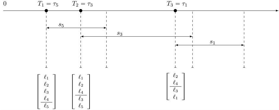
Figure 1. Sequence of defaults and the corresponding memory periods.
condition remains effective until . This is shown by a square bracket
  which indicate that the random vector
  should be sampled under the condition
at time![]() . If the second default occurred at time
. If the second default occurred at time , then the updated default threshold at
 should be sampled under the condition
 . However, at the third default time
 , investor’s interest have changed from the first default to the second default completely, i.e., the memory period of 5 after
  have finished. Therefore updated default threshold should be sampled under the condition
 . Notice also that


2.3. Default Contagion
In this subsection we see how the conditional distribution of the default threshold change at the default time.
Suppose that the first default occurred at time . Let
. Let  denote the unconditional density of
and let  denote the conditional density of
  given
given . The distributions of
 ,
,  change at
  from
from  to
to  then the default probabilities
 , which is restricted before
 , change from

to

Figure 2 and Figure 3 show the conditional distribution of  at
at  and
and  with
with
 . Distributions are truncated above the running minimum of the firm value 0.95. We see that the
  control the contagion impact effectively.
Remark 4 Giesecke [5] showed that ![]() does not admit the default intensity. Define the supermartingale
does not admit the default intensity. Define the supermartingale  with respect to
  as
as

where  then
then  can be expressed as

where  is cumulative distribution function of
 . Define the nondecreasing process
  by the Stieltjes integral

where  is the compensator of
 . Therefore

Consequently, by introducing the density function  of
of , one can obtain

which implies that  is singular because
  is concentrated on the set
 , which has
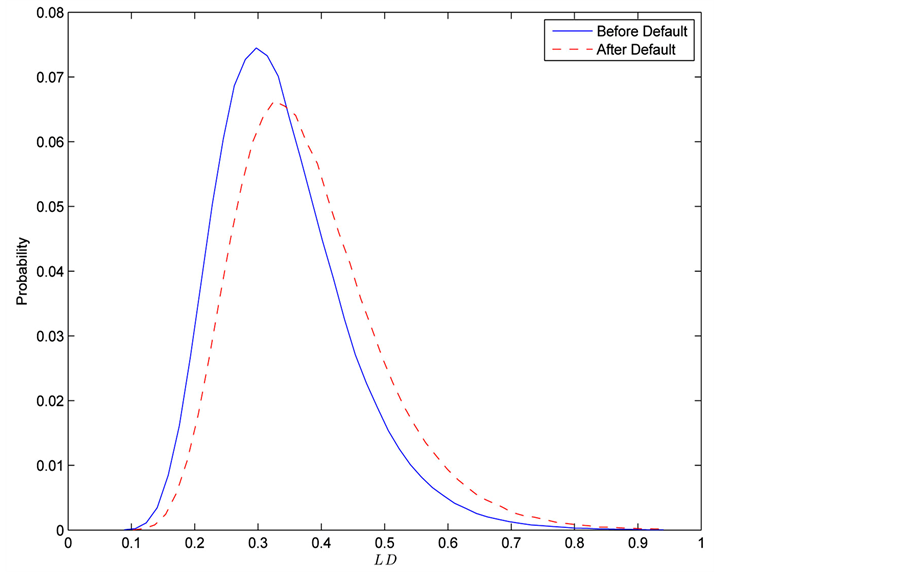
Figure 2. gi(x) and gi(x|T1 = Tj) whith rij = 0.01.
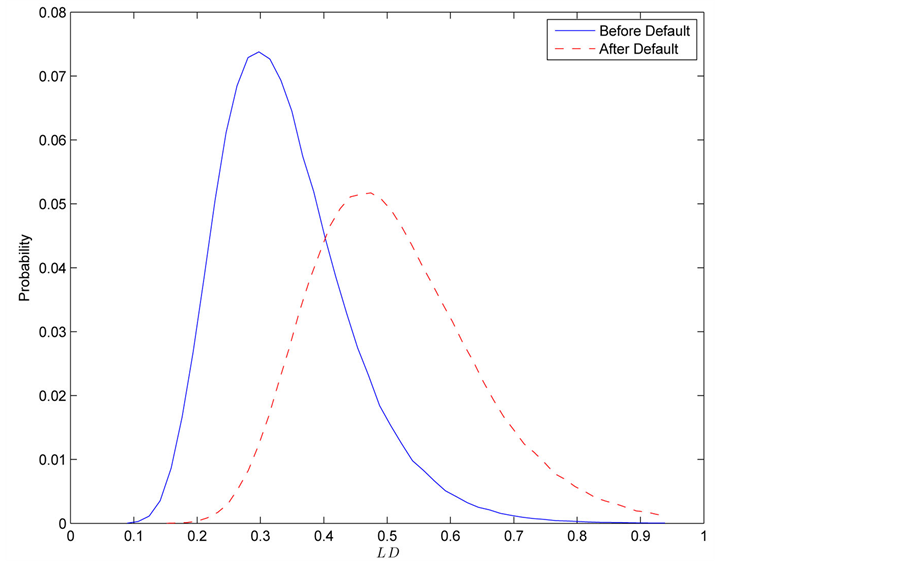
Figure 3. gi(x) and gi(x|T1 = Tj) whith rij = 0.04.
Lebesgue masure 0. Therefore  does not admit the representation
 . This is the reason why we argue the default probabilities instead of the default intensities in our model.
3. Monte Carlo Method
This section develops a numerical method to compute the distribution of the number of defaults via Monte Carlo simulation. Complicating matters is the fact that new information of defaults changes the mean and covariance of the joint distribution of the thresholds. At each moment, covariance matrix should be calculated relying upon whether the memory period have terminated or not. Therefore, the simulation depends on the path, i.e. the order of occurrence of sequential defaults.
The time interval  is partitioned into sub-intervals of equal length
 ![]() and firm value processes evolve along the discretized time step
and firm value processes evolve along the discretized time step , where
 . With the discretization of the time variable, we redefine the default time as
 (0.10)
in analogy with its continuous time version (0.3). As mentioned in Carmona, Forque and Vestal [14] , we do not have to correct for the bias introduces by the discretization of a continuous time boundary crossing problem.
Algorithm 1 To generate a one sample path of the total default , perform the following:
Step 0. Initialize ,
, . Set
. Set ,
,  ,
,  and
and . Draw the random barrier
 for all firms in portfolio and fix them until the first default occurred.
Step 1. Generate the  -dimensional path
  and calculate the running minimum
 for each
 .
.
Step 2. Determine whether default occurred or not at time  and renew the set
  as follows.
If , then the firm
  gets default at time
 , and then set
 .
.
Else, set .
.
Let  be a set consists of defaulted firms at time
  and go to Step 3.
If  hold for all
 , set
, set  for all
  and go to Step 1.
Step 3. Determine  for all defaulted firms and calculate the realized barrier for the defaulted firms and store
 .
.
Step 4. Renew the matrix  and the set
 . Draw the random barrier
  for all survived firms
  and fix them until next default occurred. Sampling is based on the distribu-tion truncated above
 .
.
Step 5. Set  and go to Step1.
4. Interacting Particle System
In credit risk management, it is important to measure how often the rare but crucial events will occur. However, standard Monte Carlo algorithm in Section 3 may be inefficient in some situations such as the portfolio constituents have small default probabilities. This is because, in order to estimate accurately the probability of rare events, a large number of trials may be required with Algorithm 3.1.
In an effort to estimate the accurate probabilities within a reasonable computational time, we embed IPS to original standard Monte Carlo simulation algorithm. In the following two subsections, we provide a quick overview of the IPS inspired by the pioneering work Del Moral and Garnier [15] and subsequent papers Carmona, Forque and Vestal [14] , Carmona and Crepey [16] and Giesecke et al. [7] .
4.1. Feynman-Kac Path Measures
Let  be the time horizon. Partition the interval
  into
into ![]() subintervals of length
subintervals of length . Let
. Let  be the discrete time Markov chain given by
  where, in our model, continuous time Markov chain
  is given by

which will be discussed later. In general, the random element  takes values in some measurable state space
 that can change with
![]() . We denote by
. We denote by  the transition kernels of the Markov chain
 at time
![]() , and we denote by
, and we denote by  the historical process of
  defined by

Next, we let  denote the transition kernels of the inhomogeneous Markov chain
![]() . We finally let
. We finally let  be the space of all bounded measurable functions on some measurable space
 , and we equip
  with the uniform norm.
The Interacting Particle System consists of a set of  path-particles
  evolving from time
 to
to . The initial generation at time
  is a set of independent copies of
  and the system evolves as if strong animals produce many offsprings, however the rest die.
For each , we consider non-negative measurable functions
  defined on
  equipped with the product
 ![]() -algebra, and we call these functions as potential functions. We associate to the pair of potentials and transitions
-algebra, and we call these functions as potential functions. We associate to the pair of potentials and transitions  the Feynman-Kac path measure defined for any test function
  by the formula
 (0.11)
We also introduce the corresponding normalized measure
 (0.12)
Note that

Therefore, for any given bounded measurable function , we have
 (0.13)
The above relationship has the merit of relating the un-normalized expectations in the left hand side to normalized expectations in the right hand side. Furthermore, for any path , we define the weighted indicator function

Then we see that
 (0.14)
This formula can be applied to the situation that the  are the rare events and it can be computed via computation of normalized measures. It is known (see Del Moral and Garnier [15] ) that the computation of the sequence of normalized measures is achieved by the following non-linear recursive equation
 (0.15)
starting from . Equation (0.15) has the differential form

which can be easily seen by substituting

and

into the integrand of the right hand side of (0.15).
4.2. Interacting Particle Interpretation
For the purpose of numerical computations of the rare events of the form (0.14), we introduce an interacting particle system. We choose a large integer  which we shall interpret as the number of particles. We construct a Markov chain
  whose state
  at time
 ![]() can be interpreted as a set of
can be interpreted as a set of  samples of particles with respect to the measure
 ,
,

We start with an initial configuration  that consists of
  independent and identically distributed random samples from the distribution

i.e.,  where the
  are drawn independently of each other from the distribution
 . The transitions of particles from
  into
into  are defined by
 (0.16)
where  is the empirical measure defined by

and  represents an infinitesimal neighborhood of the point
 . By the definition of
 , one sees that (0.16) is the superposition of two identifiable transitions, a selection followed by a mutation as shown below.

The selection stage is performed by choosing randomly and independently  particles

according to the Boltzmann-Gibbs measure

During the mutation stage, each selected particle  is extended in time by an elementary
  -transition.
In other words, we set

where  is a random variable with distribution
 . The mutations are performed independently.
A result of [17] reproduced in [15] states that for each fixed time![]() , the empirical measure converges in distribution, as
, the empirical measure converges in distribution, as , toward the normalized Feynman-Kac measure
 , i.e.,
 (0.17)
Mimicking (0.13), unbiased particle approximation measures  of the un-normalized measure
  are defined as

and then, by (0.14), we can get the particle approximation of the rare event probabilities. More precisely, if we let

then  is an unbiased estimator of the rare event probabilities
  such that
 (0.18)
We refer to Del Moral [17] and Del Moral and Garnier [15] for the details of the convergence results. Their complete proofs rely on a precise propagation of chaos type analysis and they can be found in Section 7.4 on Pages 239-241 and Theorem 7.4.1 on Page 232 in Del Moral [17] .
4.3. IPS Algorithm and Potential Functions
We introduce special notations  and
and  which indicate that these are the input to the selection stage, while another notation
  and
and  indicate that these are the input to the mutation stage of the IPS algorithm. Here, as we will describe later,
  indicate the parent of
 .
.
According to Del Moral and Garnier [15], one of the recommended potential functions are of the form
 (0.19)
for some  and suitable function
  so as to satisfying

This regularity condition ensures that the normalizing constants  and the measure
  are bounded and positive. Thanks to the form of this potential function, we note that we need only to keep track of
  and
and , and then the selection would be implemented with those two particles. The form of the distribution (0.17) shows that in order to have more simulation paths realizing great many defaults, it is important to choose a potential function becoming larger as the likelihood of default increases. To meet our purpose, we choose the function
  as follows.
 (0.20)
Then our potential function is given by
 (0.21)
The first term of (0.21) reflects the fact that the high weights are assigned to the particle which had renewed the running minimum during the period . When
  is not random, i.e., the default barrier is observable, it is known that the IPS is effective to simulate the counting process
  with reasonable accuracy by Carmona, Fouque and Vestal [14] . We borrowed the form of potential function from Carmona, Fouque and Vestal [14] . Detailed IPS algorithm is summarized as follows.
Algorithm 2 Assume that we have a set of  particles at time
 ![]() denoted by
denoted by . We define the Markov process

where , and define the discrete time Markov process
 .
.
To generate an estimate of  for
for , perform the following:
Step 0. Initialize the particles  and indicators
 . Choose
  as a discretized time step for the firm value processes, to be some small value. We start with a set of
  i.i.d. initial conditions
 chosen according to the initial distribution of
 .
.
Set  (initial value of
 ) for all
  and then form a set of
  particles
 .
.
Step 1. For each step , repeat the following steps.
• Selection.
Compute the normalizing constant
 (0.22)
and choose independently  particles according to the empirical distribution
 (0.23)
The new particles are denoted by .
.
• Mutation.
For every , using the Algorithm 3.1, the particle
  is transformed into
 independently by
 (0.24)
and set .
.
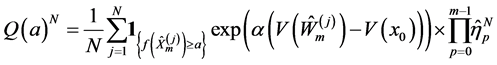
Step 2. The estimator of the probability  is given by
 (0.25)
It is known that this estimator is unbiased in the sense that  and satisfies the central limit theorem. (Refer to [15] [17] )
Instead of explicit calculation of the asymptotic variance, we notice that the approximate variance 
defined by
 (0.26)
can be easily calculated within the above IPS algorithm. This provides criteria to choose the parameter  to be a suitable level.
5. Numerical Examples
This section demonstrates the performance of the IPS algorithm through numerical examples with a sample portfolio consists of 25 firms. We consider portfolio consisting of high credit quality names with high correlations  of their firm value processes, as well as high correlations
  of the default thresholds. The parameters of the model are summarized as follows.
•  for all
 •
•  for
for  and
and ,
,  for
for  and
and .
.
Those parameters are set with the intention to notice rare default events. As Carmona, Fouque and Vestal [14] reports, the number of selections/mutations which is equal to ![]() in Algorithm 4.1 will not have so significant impact to numerical results then we set
in Algorithm 4.1 will not have so significant impact to numerical results then we set  per one year. Here we set
 .
.
First we compare the results of the IPS algorithm to the results obtained by the standard Monte Carlo algorithm in case of  years. For the standard Monte Carlo, we run 10,000 trials and in addition, 500,000 trials that will be expected to achieve reasonably accurate values. As for IPS algorithm, we set
  and
and  and take
  for number of the particles. Figure 4 illustrates the probability of defaults
 for
for  for
for  with
with  for all
 . Thus the market participants memorize all the default by the time horizon. Figure 5 plot the log scale for these three cases of probabilities for comparison. One can see that the standard Monte Carlo with 10,000 trials has oscillating results for rare events although the IPS results shows similar shape as 500,000 trials of Monte Carlo. For this numerical calculation, 500,000 trials took about 8000 seconds, whereas the IPS algorithm took about 275 seconds with 3.4 GHz Intel Core i7 processor and 4 GB of RAM.
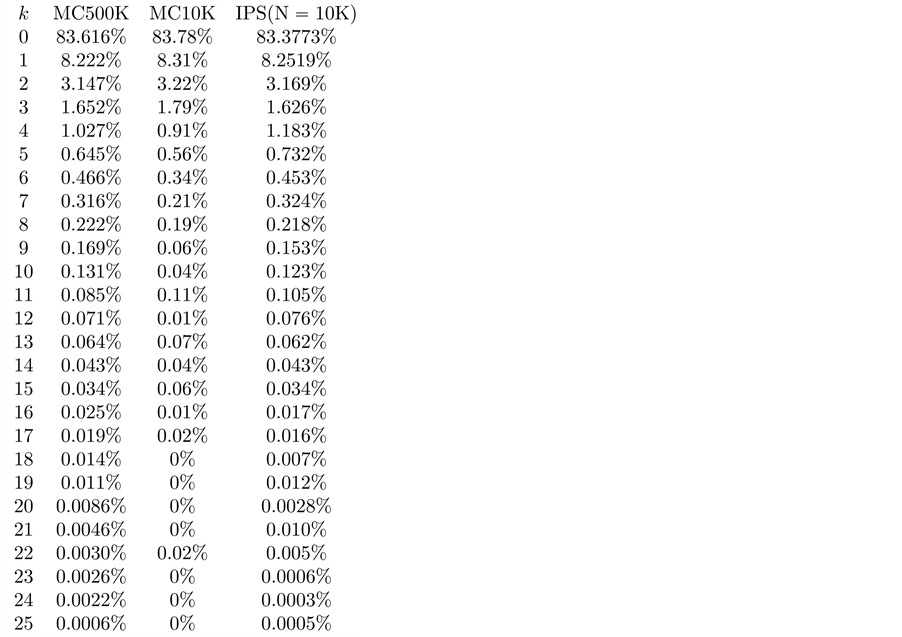
Figure 4. Default probabilities.
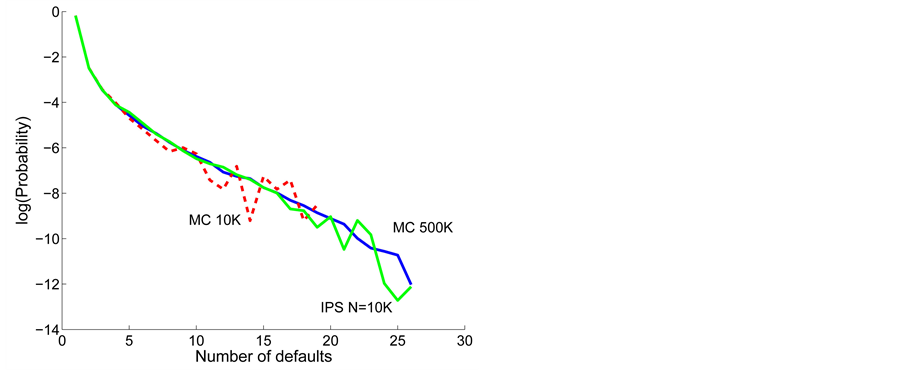
Figure 5. Default probabilities in log-scale.
These numerical results show that the standard Monte Carlo with 10,000 trials can not capture the occurrence of rare default events such as over 20 defaults, however, one sees that there exist very small probabilities for such events via 500,000 trials which is indicated by solid blue line in Figure 5. As expected, IPS algorithm can capture these rare event probabilities which are important for the credit risk management.
Next, we investigate how variance would reduced by IPS with following two cases
• Case 1:  and
and  for all
 • Case 2:
  and
and  for all
 to see the difference with respect to time horizon with the same memory period. Preliminary version of this paper, Takada [11] illustrated how the default distributions change in response to the memory period
 ![]() based on the standard Monte Carlo. One sees that the first default occurs with the same probability for different
based on the standard Monte Carlo. One sees that the first default occurs with the same probability for different  s but the second default occurs with different probability because contagion effects are different in response to the memory period
![]() ; The larger the memory periods get, the more tail gets fat.
; The larger the memory periods get, the more tail gets fat.
In contrast, current study focuses on how the variance is reduced with IPS algorithm compared to the standard Monte Carlo. Due mainly to the computation of sampling with replacement according to the distribution (0.23) in the selection stage, IPS algorithm generally requires more time than the standard Monte Carlo. Although it obviously depends on input parameters, with the above parameter set of 25 names and in case of , the calculation in IPS took approximately 1.03 times longer than that of standard Monte Carlo. Thus, in the rest of the paper, for comparison for accuracy, we take the number of trials in Monte Carlo equals to the number of the particles in IPS. In order to see the effectiveness of the IPS, we run both the Monte Carlo with
  trials and the IPS with
  particles for 1000 times for each, and then compare the sample standard deviation of the 1000 outcomes of the probabilities
  for all
  More specifically, let
 be
be  -th outcome of
  obtained by the standard Monte Carlo and
  be
be  -th outcome of
  obtained by the IPS. Calculate the sample standard deviation of
 , denoted by
 , and also calculate the sample standard deviation of
 , denoted by
 . Finally compare the two values
  and
and  for each
 and then we see which algorithm achieves low standard deviation. Figure 6 and Figure 7 illustrate the differences between
  and
and  in Case 1.
And figure 8 and figure 9 illustrate the differences between  and
and  in Case 2.
Remarkable feature is that the IPS algorithm reduces variance for the rare events, i.e., more than 10 defaults in our example, while instead, demonstrates weak performance for . Therefore, whether to chose IPS depends on the objective and its assesment(division) might depends on the portfolio and the parameters. Thus, although we need several trial runs for the first time with given portfolio, once we get the suitable control parameters such as
 , reliable results would be obtained.
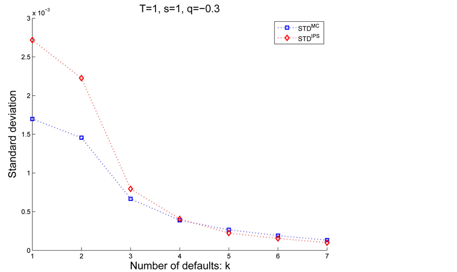
Figure 6. Case 1: 1 ≤ k ≤ 7.
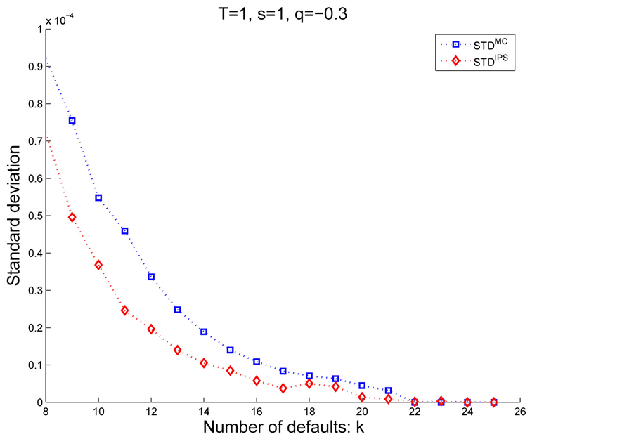
Figure 7. Case 1: 8 ≤ k ≤ 25.
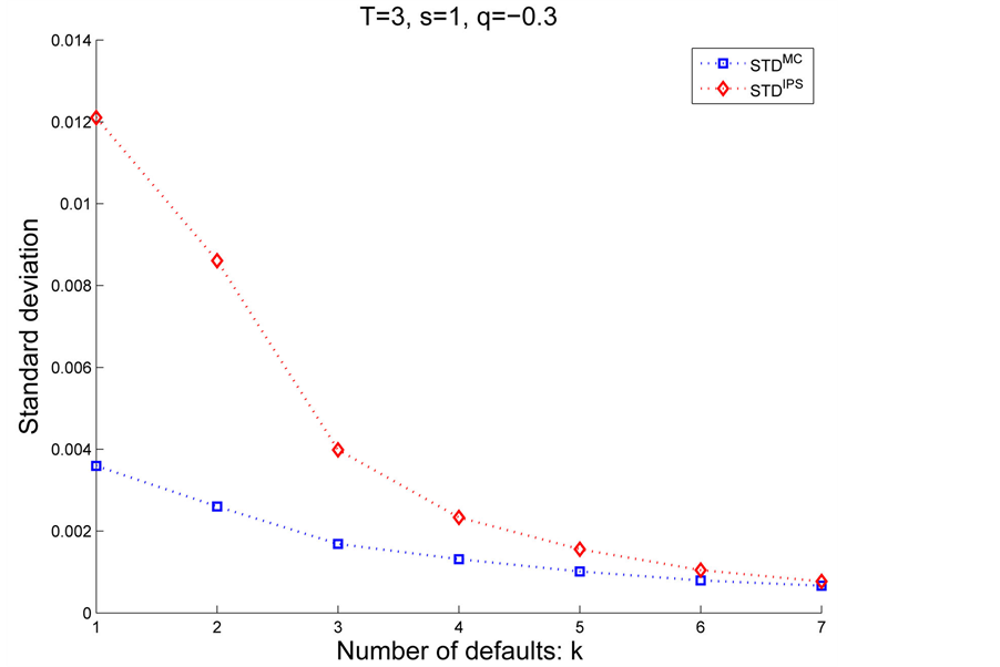
Figure 8. Case 2: 1 ≤ k ≤ 7.
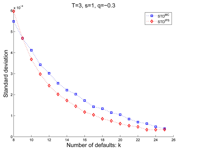
Figure 9. Case 2: 8 ≤ k ≤ 25.
6. Conclusion
This paper proposed incomplete information multi-name structural model and its efficient Monte Carlo algorithm based on the Interacting Particle System. We extend naturally the CreditGrades model in the sense that we consider more than two firms in the portfolio and their asset correlation as well as the dependence structure of the default thresholds. For this purpose, we introduced the prior joint distribution of default thresholds among the public investors described by truncated normal distribution. Numerical experience demonstrated that the IPS algorithm can generate rare default events which normally requires numerous trials if relying upon a simple Monte Carlo simulation. Finally we verified the IPS algorithm reduces variance for the rare events.
Acknowledgements
The author is grateful to participants of the RIMS Workshop on Financial Modeling and Analysis (FMA2013) at Kyoto and participants of the Quantitative Methods in Finance 2013 Conference (QMF 2013) at Sydney for valuable comments which helped to improve this paper.
References
- Davis, M. and Lo, V. (2001) Infectious Defaults. Quantitative Finance, 1, 382-387.
- Yu, F . (2007) Correlated Defaults in Intensity Based Models. Mathematical Finance, 17, 155-173.
- Frey, R. and Backhaus, J. (2010) Dynamic Hedging of Synthetic SDO Tranches with Spread and Contagion Risk. Journal of Economic Dynamics and Control, 34, 710-724.
- Frey, R. and Runggaldier, W. (2010) Credit Risk and Incomplete Information: A Nonlinear-Filtering Approach. Finance and Stochastics, 14, 495-526. http://dx.doi.org/10.1007/s00780-010-0129-5
- Giesecke, K . (2004) Correlated Default with Incomplete Information. Journal of Banking and Finance, 28, 1521-1545.
- Giesecke, K . and Goldberg, L. (2004) Sequential Defaults and Incomplete Information. Journal of Risk, 7, 1-26.
- Giesecke, K., Kakavand, H., Mousavi, M. and Takada, H. (2010) Exact and Efficient Simulation of Correlated Defaults. SIAM Journal of Financial Mathematics, 1, 868-896.
- Schönbucher, P. (2004) Information Driven Default Contagion. ETH, Zurich.
- Takada, H. and Sumita, U. (2011) Credit Risk Model with Contagious Default Dependencies Affected by MacroEconomic Condition. European Journal of Operational Research, 214, 365-379.
- McNeil, A., Frey, R. and Embrechts, P. (2005) Quantitative Risk Management: Concepts, Techniques and Tools. Princeton University Press, Princeton.
- Takada, H. (2014) Structural Model Based Analysis on the Period of Past Default Memories. Research Institute for Mathematical Sciences (RIMS), Kyoto, 82-94.
- Finger, C.C., Finkelstein, V., Pan, G., Lardy, J., Ta, T. and Tierney, J. (2002) Credit Grades. Technical Document, Riskmetrics Group, New York.
- Fang, K., Kotz, S. and Nq, K.W. (1987) Symmetric Multivariate and Related Distributions. CRC Monographs on Statistics & Applied Probability, Chapman & Hall.
- Carmona, R., Fouque, J. and Vestal, D. (2009) Interacting Particle Systems for the Computation of Rare Credit Portfolio Losses. Finance and Stochastics, 13, 613-633. http://dx.doi.org/10.1007/s00780-009-0098-8
- Del Moral, P. and Garnier, J. (2005) Genealogical Particle Analysis of Rare Events. The Annals of Applied Probability, 15, 2496-2534. http://dx.doi.org/10.1214/105051605000000566
- Carmona, R. and Crepey, S. (2010) Particle Methods for the Estimation of Credit Portfolio Loss Distributions. International Journal of Theoretical and Applied Finance, 13, 577. http://dx.doi.org/10.1142/S0219024910005905
NOTES

*Corresponding author.