Journal of Mathematical Finance
Vol.3 No.3(2013), Article ID:35896,9 pages DOI:10.4236/jmf.2013.33038
Dynamics of Entrepreneurship under Regime Switching
1School of Finance, Shanghai University of Finance and Economics, Shanghai, China
2Shanghai Key Laboratory of Financial Information Technology, Shanghai, China
Email: shasha1989123@hotmail.com, yang.jinqiang@mail.sufe.edu.cn, liminghui02@gmail.com
Copyright © 2013 Sha Sun et al. This is an open access article distributed under the Creative Commons Attribution License, which permits unrestricted use, distribution, and reproduction in any medium, provided the original work is properly cited.
Received May 30, 2013; revised July 6, 2013; accepted July 18, 2013
Keywords: Regime Switching; Entrepreneurial Finance; q Theory of Investment; Liquidity Constraints; Precautionary Saving
ABSTRACT
We propose a tractable model of entrepreneur dynamics where the investment conditions are stochastic. Applying the approach of stochastic control and optimization, we solve the dynamics of the entrepreneur’s optimal investment, consumption and portfolio allocation under regime switching. We find that the interactions of precautionary savings and liquidation boundary advance/postpone motives generate rich implications for entrepreneur dynamics. Facing the threat of financial crisis, entrepreneurs build cash reserves and bring forward liquidation option exercise to mitigate downside risk. During the bad times, entrepreneurs value financial slack and postpone liquidation boundary to maintain the business and wait for the good state to come.
1. Introduction
The ability of regime-switching models to capture the cyclical features of real macroeconomic variables as proposed by Hamilton [1] is widely accepted. Since then, there has been growing interest in applications of regime-switching models into a wide class of financial and economic problems (see Honda [2], Guo, Miao, Morellec [3] among others). It’s reasonable to believe that firm policy can be affected by regime shifts, since booms and recessions can have significant impact on the profitability or riskiness of both real and financial investment and the willingness to consume. Recent empirical studies show that firms’ financing and investment behaviors change dramatically during the 2008 financial crisis (see Campello, Graham and Harvey [4], Ivashina and Scharfstein [5]). However, little theoretical research has been done on the relation between regime switching and the dynamics of entrepreneur’s optimal consumption, investment and portfolio allocation. In this paper, we try to focus on the following interesting questions: How should entrepreneurs choose optimal consumption, investment, portfolio allocation and liquidation boundary when facing the threat of financial crisis in the future? How should entrepreneurs behave during a financial crisis?
To address these questions, we propose a quantitative model to study the dynamics of entrepreneur’s optimal consumption, investment and portfolio allocation when the dynamics of decision variables are subject to discrete regime shifts at random times. Our model builds on the dynamic framework of entrepreneur’s optimal policies (see Wang, Wang and Yang [6], henceforth WWY) by adding stochastic investment conditions. We have shown that when the entrepreneur faces uncertain macro conditions, it is optimal for them to hoard cash for precautionary reasons. In addition, the entrepreneur may choose the optimal liquidation boundary to eliminate the risk associated with regime switching. The analysis shows that precautionary savings and liquidation boundary advance/ postpone can have significant value and generate rich implications for entrepreneur dynamics.
The analysis in the present paper relates to two different strands of literature. First, it relates to the entrepreneurship literature. Hurst, Lusardi [7] used empirical methods to show that liquidity constraint induces the entrepreneur to initiate small-sized business. Herranz, Krasa and Villamil [8] studied the entrepreneur’s behavior from the aspect of law, and found that the more riskaverse the entrepreneur, the more likely he executes liquidation option. Chen, Miao and Wang [9] developed a dynamic incomplete-market model of entrepreneurial firms building on Leland [10] and presented the implications of nondiversifiable risks on entrepreneurial finance. Hall and Woodward [11] studied the risk facing venture capital-backed entrepreneurial firms. Wang, Wang and Yang [6] proposed an incomplete-market q-theoretic model to study entrepreneurial dynamics, and found that precautionary motive, borrowing constraints, and capital illiquidity lead to underinvestment, conservative debt use, under-consumption, and less risky portfolio allocation. However, all these models assume that investment conditions are time-invariant.
Second, the present paper relates to a series of recent papers on regime switching. Driffill, Kenc, Sola [12] modeled the underlying asset return dynamic as a regime switching process to value a perpetual American call option. Honda [2] defined an unobservable regime variable in the economy as a continuous-time Markov chain and studied dynamic optimal consumption and portfolio choice in which the mean return of a risky asset shifts between regimes. Guo, Miao, Morellec [3] proposed a real option model in which the growth rate and volatility of the decision variable shift between different states at random times, and the results showed investment is intermittent and increases with marginal q under this policy. Chen [13] built a dynamic capital structure model and demonstrated how business cycle variations in expected growth rates, economic uncertainty, and risk premia influence firm’s financing policies. One of our main contributions is the extensions of regime switching settings to the study of entrepreneurial dynamics, which includes entrepreneur’s optimal consumption, investment and portfolio allocation decisions.
The paper that is most closely related to the present analysis is Bolton, Chen and Wang [14] (henceforth BCW). The authors analyzed dynamic corporate financial management for a financially constrained risk-neutral firm under stochastic financing conditions. They found that firms have precautionary cash hoarding and market timing motives to mitigate macroeconomic risk. One essential difference between the two papers is that we examine the dynamics of entrepreneurship while they focus on financially constrained public firms. Another important point of departure is that we assume stochastic investment conditions, whereas they consider stochastic financing conditions. Finally, we use nonexpected recursive utility function to separate risk aversion from the elasticity of intertemporal substitution (EIS). However, they consider risk-neutral pricing.
The remainder of the paper is organized as follows. Section 2 presents the model of entrepreneur dynamics under regime switching. Section 3 derives the model solution. Section 4 presents parameter choices and quantitative results. Section 5 concludes.
2. The Model
In this section, we propose our quantitative model to study the dynamics of entrepreneurship under regime switching. Our model is built on WWY [6] by adding stochastic investment conditions. In particular, we assume the economy has two aggregate states,  (boom and recession). The state
  follows a continuous-time Markov chain alternating between state G and B and the transition intensity follows a Poisson law. Let
  denote the transition intensity from state
  to state
 . Then the probability of the economy switching from state G to state B within a small period
  is approximately equal to
 , while the probability of switching from state B to G is approximately
 . In our model, parameters related to investment conditions, i.e.
  and
and , and liquidation value
  take different values when the process
  is in different states.
Stochastic investment conditions and production technology. The entrepreneur employs only capital and cash as the factor of production. We denote  as the gross investment and
  as capital stock. As is standard in capital accumulation models, the change of capital stock
  evolves according to
 (1.1)
(1.1)
where  is the rate of depreciation.
We assume the cumulative productivity shock  follows arithmetic Brownian motion process. Thus, the firm’s productivity shock
  over the period
  is given by
 (1.2)
(1.2)
where  is a standard Brownian motion,
  is the mean of the productivity shock in state
 , and
, and  is the volatility of the productivity shock in both states.
The firm’s operating revenue over period  is given by
 . After investment
  and adjustment cost
 , the firm’s operating profit
  over the same period is given by
 (1.3)
(1.3)
where the price of the investment good is set to unity and  is the adjustment cost.
Following Hayashi [15], we assume that the firm’s adjustment cost  is homogeneous of degree one in
  and
and . And adjustment cost
  is written in the following homogeneous form
 (1.4)
(1.4)
where  is the firm’s investment-capital ratio and
  is an increasing and convex function. To make the analysis simple and tractable ( see WWY [6], BCW [14] for example), we assume that
 (1.5)
(1.5)
where the parameter  measures the degree of the adjustment cost. The higher
 , the more adjustment cost occurs.
Finally, the entrepreneur can liquidate its assets at any moment. The flexibility of liquidation option makes the entrepreneur optimally manage his downside business risk. Liquidation gives a terminal value , where
  depends on the state
 . A higher
  implies a higher liquidation value. Obviously, we have
 , which makes liquidation in the good state much more attractive than in the bad state. Let
  denote the entrepreneur’s optimally chosen liquidation time.
Financial investment opportunities. In our model, the entrepreneur has financial investment opportunities to partially hedge his business risk. The entrepreneur allocates his liquid financial wealth between a risk-free asset which pays a constant rate of interest  and the risky market portfolio (Merton [16]). The incremental return
  of the market portfolio over time period dt evolves as follows,
 (1.6)
(1.6)
where  is the mean of the market portfolio return in state
  and
and  is the volatility of the market portfolio return in both states, and B is a standard Brownian motion. The correlation coefficient
  between
  and
and  is less than 1, which implies there exists nondiversifiable risk and the entrepreneur can’t completely hedge his business risk. Let
  denote the Sharpe ratio of the market portfolio in state
 , which is given by
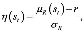 (1.7)
(1.7)
We denote  and
and  as the agent’s financial wealth and the amount invested in the risky asset respectively. Given the entrepreneur’s operating profit, investment, consumption and portfolio allocation, we can write the dynamics of liquid financial wealth
  as follows:
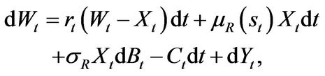 (1.8)
(1.8)
where the firm term is the return on risk-free asset, the second and third terms are the return on market portfolio, the fourth term  is the entrepreneur’s consumption, and the last term
  is the firm’s cash flows from operations.
We assume the entrepreneur can use capital  as collateral to borrow and the borrowing is risk-free. Thus, the liquidation value of capital
  must be greater than outstanding liability. So the following Equation holds,
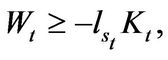 (1.9)
(1.9)
The Entrepreneur’s Objective. The entrepreneur maximizes his utility defined as,
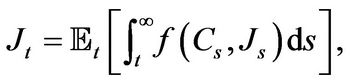 (1.10)
where  for Epstein-Zin non-expected homothetic recursive utility (Duffie and Epstein [17]) is given by
 (1.11)
where
 (1.12)
In the above utility function, the parameter  is the elasticity of intertemporal substitution (EIS), and the parameter
  is the coefficient of relative risk aversion. The parameter
  is the agent’s subjective discount rate. To maximize his utility, the entrepreneur chooses investment, consumption and portfolio allocation subject to the collateralized borrowing limit (1.9). And the agent optimally chooses the liquidation time
 .
.
3. Model Solution
The entrepreneurial value depends on both its capital stock  and its cash holdings
 . Thus, let
  denote the value function in state
 . It satisfies the following system of Hamilton-Jacobi-Bellman (HJB) Equations:
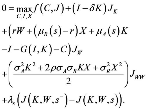 (1.13)
The first term on the right side of the HJB Equation (1.13) represents the one-period utility. The second term represents the effect of capital stock changes on entrepreneurial value. The third and fourth terms represent the effect of the expected change in cashing holdings  and volatility of
  on entrepreneurial value and the last term is the expected change of entrepreneurial value when the state changes form
  to
to .
.
Next, we solve the first-order conditions (FOC) with respect to consumption , investment
  and portfolio choice
  respectively. The FOC with respect to consumption
  is
is
 (1.14)
which shows the marginal utility of consumption  is equal to the marginal utility of wealth
  at optimality.
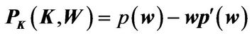
The FOC with respect to investment  is given by
 (1.15)
which implies the entrepreneur’s marginal cost of investing  is equal to the marginal benefit of adding a unit of capital
  in state
 .
.
The FOC with respect to portfolio choice  is given by
 (1.16)
which states that the optimal amount investing in market portfolio is equal to the mean-variance demand (the first term on the right side) plus the hedging demand (the second term).
Then, we conjecture that the value function  is given by
 (1.17)
where  is given in appendix B and
  is the entrepreneur’s certainty equaivalent (CE) wealth.
Using the homogeneity property, we can write scaled CE wealth as  in each state. We substitute the FOCs with respect to
 ,
,  ,
,  , the value function form and the scaled CE wealth into the HJB Equation (1.13), and then get the systems of ordinary differential Equations (ODE) for scaled CE wealth
 . The results are summarized in the following theorem.
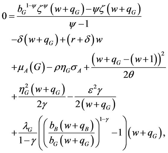
Theorem 1 The scaled CE wealth  solves the following system of ODEs,
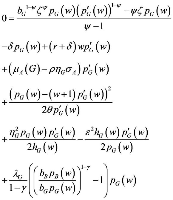 (1.18)
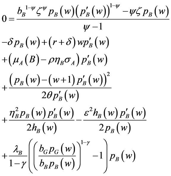 (1.19)
where  is given by
 (1.20)
and  is given by
 (1.21)
Intuitively,  can be referred to as the idiosyncratic component of the total volatility of the productivity shock and
  is the effective risk aversion (see WWY [6]).
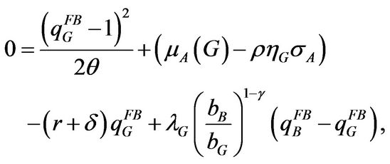
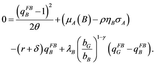
Next, we specify the boundary conditions. When  approaches infinity,
  approaches the first-best solution given by
 (1.22)
where  is calculated in the appendix B.
At the endogenous liquidation boundary, we have the following value matching and smooth pasting conditions for ,
,
 (1.23)
 (1.24)
Finally, the optimal scaled consumption , investment
 , and market portfolio allocationcapital ratio
  are given by
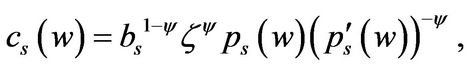 (1.25)
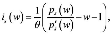 (1.26)
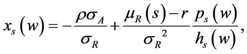 (1.27)
where  is the marginal value of cash in state
 .
.
4. Quantitative Results
In this section, we illustrate the quantitative results for given parameter choices of the model. First, we specify our choice of parameters. In state G, the expected productivity is set to be  (Eberly, Rebelo, and Vincent [18]), while in state B
  is set to be 18% to reflect the worse investment condition in the bad state. Similarly, the mean return of market portfolio is set as
  and
and . We choose the liquidation parameter
  in state G in line with estimates provided by Hennessy and Whited [19]. In the bad state, the capital liquidation value is set to
  to reflect the severe lack of liquidity during a financial crisis. The transition intensity out of state G is set at
 , which implies an average duration of 10 years for good times. The transition intensity out of state B is
 , with an implied average length of a financial crisis being 2 years. This reasonable setting is borrowed from BCW [14].
The other parameters remain the same in the two states, and we set the parameters by widely-used numbers (see WWY [6]). The risk-free interest rate is . The subjective discount rate is set to equal to the risk-free rate,
 . We obtain the adjustment cost parameter
  and the rate of depreciation for capital stock
  The volatility of productivity shocks
  is
is  (Eberly, Rebelo, and Vincent [18]) and the volatility of return on market portfolio
  is
is . We consider widely used values for the coefficient of relative risk aversion,
  and we set the EIS to be
 .
.
4.1. Entrepreneur Welfare and Optimal Liquidation Boundary
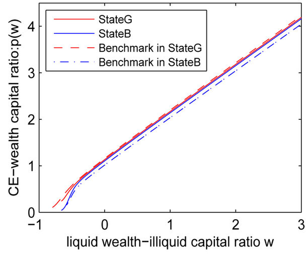
Figure 1 plots entrepreneur’s CE wealth , average
  and net marginal value of cash
  and marginal value of capital
  in both states. For all panels, we graph both the transitory two states and the benchmarks in two states with transitory intensity equaling to zero. Since
 ,
,  and
and  conveys the same information and
  is easier to read, we discuss
 . As expected, average q in state G is higher than in state B. More remarkable is the fact that the difference between the average q in the two states is so large especially for lower levels of cash holdings. However, this phenomenon is not that obvious in the benchmarks. This difference in average q is due to differences in investment conditions.
In state G, the optimal liquidation boundary 
 . At this point, the firm hasn’t reached the boundary compared with the benchmark. Further running the business would help the entrepreneur earn more profit. However, doing so would mean taking the risk that the state of nature switches to the bad state when the investment condition is much worse. The entrepreneur makes the trades off and optimally exercises the liquidation option by liquidating when
  hits the lower barrier
 . However, the optimal liquidation boundary
 in state B is lower than the benchmark, which implies that the firm struggles to maintain the business and waits for the possible arrival of good state.
Panel C of Figure 1 underscores the significant impact of stochastic investment conditions on the marginal value of cash. The entrepreneur with low cash holdings values cash more in the bad state. In our model, the marginal value of cash in state B reaches , almost double
  in the good state, when
 . When
 ,
,  in four scenarios all approaches to
 .
.
Comparing the transitory case with the benchmark case,  displays different dynamics. In good state, for an entrepreneur with sufficient financial slack,
  is higher than the benchmark, since wealth can mitigate the additional risk associated with regime switching. For an entrepreneur with low financial slack,
  is lower than the benchmark.
However, in the bad state, the entrepreneur values his cash more than in the benchmark, no matter his financial slack is sufficient or not. Intuitively, the entrepreneur may value wealth less, aware of the possibility of the state of nature switching to the good state. It is incorrect, because the entrepreneur needs more cash to maintain the business and postpone the liquidation option exercise.
Panel D plots marginal value of capital , which is also referred to as the marginal
 . The entrepreneur with medium cash holdings values capital more in the bad state and the one with extreme low (near the liquidation boundary) and high cash holdings values capital more in the good state. When
 , the marginal
  approaches to average
  shown in Panel B.
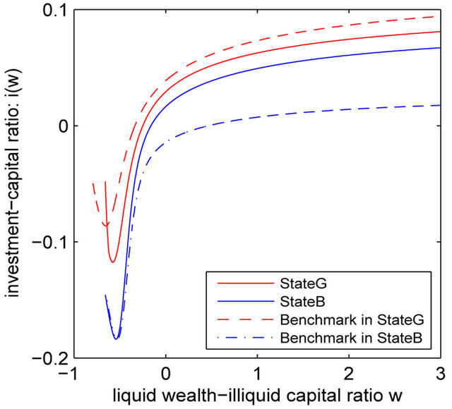
4.2. Optimal Investment
Figure 2 plots investment-capital ratio  and investment-liquidity sensitivity
 . The investment in the good state is higher than in the bad state for a give
  and the difference is especially large when
  is low. The entrepreneur’s precautionary motive is stronger in bad times, so that we should expect to see the firm hoarding more cash. This is reflected in the lower levels of investment. From Panel A of Figure 2, it can be seen that the firm engages in large asset sales and divestment up to 12% and 18% of its capital in the good and bad states respectively for cash hoarding purpose.
Compared to the benchmark, investment in the good state is lower for the entrepreneur with sufficient financial slack. Aware of the threat of switching to the bad state, the entrepreneur cuts investment and hoards cash for precautionary purpose. However, the entrepreneur
 (a)
(a)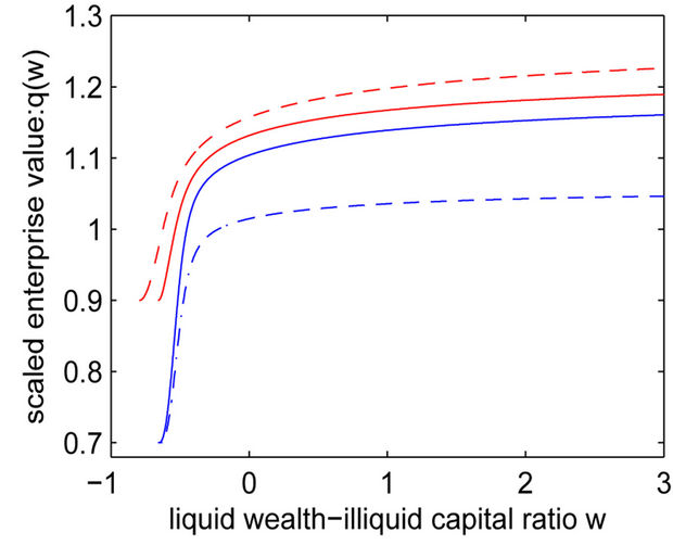 (b)
(b)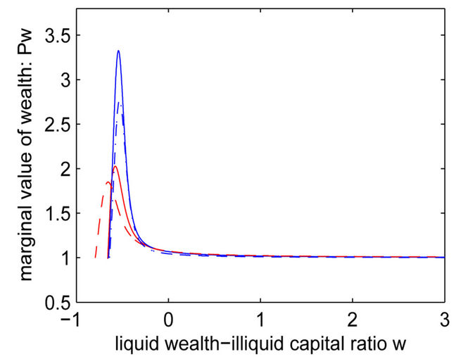 (c)
(c)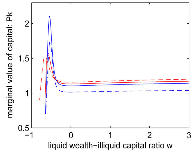 (d)
(d)
Figure 1. The entrepreneur’s scaled certainty equivalent wealth , private average
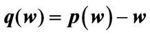 , private marginal value of liquid wealth
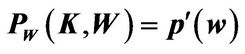 , and private marginal
 ,
, . All parameter values are given in Section “Quantative Results”.
 (a)
(a)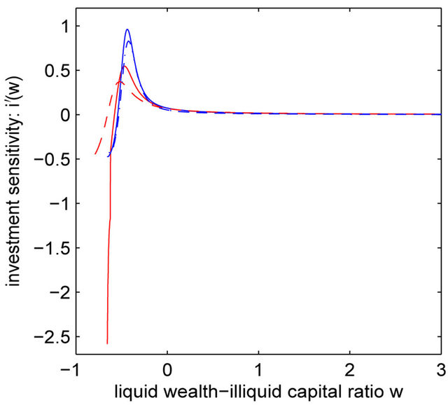 (b)
(b)
Figure 2. Investment-capital ratio  and investment-liquidity sensitivity
 . All parameter values are given in Section “Quantative Results”.
reduces disinvestment and even boosts investment to the level higher than the benchmark near the liquidation boundary. When  is near the liquidation boundary, the cash hoarding motive is dominated by the early liquidation option exercise motive, thus leading to the investment boost. In the bad state, the investment is higher than the benchmark since the possible arrival of the good state. Similarly, the investment in state B in lower than the benchmark when
  is sufficiently low. Having the possibility of the state of nature switching to the good state in mind, the entrepreneur cuts investment to maintain the business and wait for the good state to come.
Panel B of Figure 2 shows the significant impact of regime switching on investment sensitivity in both states. Obviously,  reaches down to −2.5 when
 . As the firm approaches the liquidation boundary
 , it may choose to accelerate investment aggressively (and thus reduce under-investment) to take advantage of the higher investment conditions. In state B,
  also reaches negative value near the liquidation boundary, which reveals the convexity character brought by the liquidation option.
4.3. Optimal Portfolio Allocation and Consumption
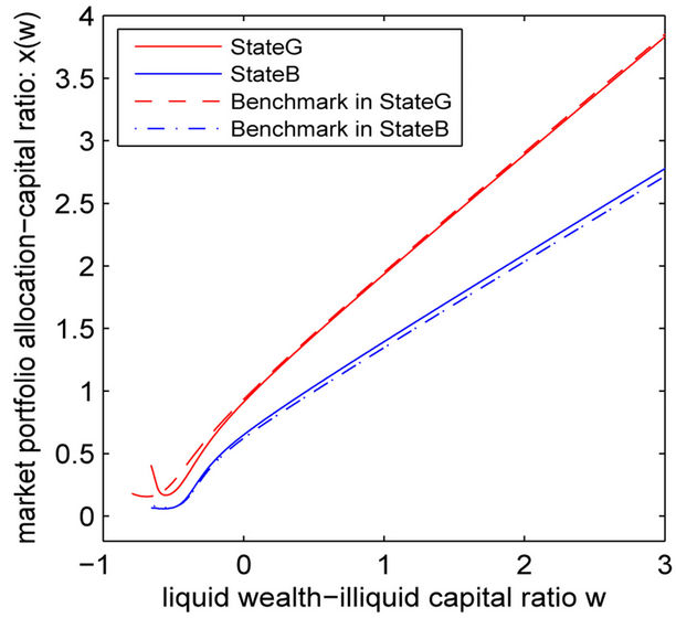
Panel A of Figure 3 plots the demand for the market portfolio  and Panel B plots the consumption
 . It’s easy to find that the graphs of Panel A and B are very similar.
As expected, the portfolio allocation in the good state is higher than the portfolio allocation in the bad state and so does consumption. Similar to the investment, the entrepreneur chooses to accelerate consumption and financial investment when the firm approaches the liquidation boundary. Strikingly,  and
and  decrease as w increases near the liquidation boundary, which is counterintuitive.
In fact, the entrepreneur needs to burn cash to bring forward the liquidation option exercise. In the bad state, the difference between 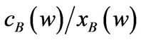 and the benchmark when w is large is significantly larger than that when w is near the liquidation boundary. Intuitively, the entrepreneur needs to hoard cash to postpone the liquidation option exercise.
Apparently, the impact of regime switching on portfolio allocation and consumption is different. Comparing Panel A and Panel B in Figure 3, one can find that portfolio allocation  in the transitory case is so close to the one in the benchmark case, except for the part near the liquidation boundary. However, the consumption experiences a large jump in both states between the transitory case and the benchmark case. Intuitively, it implies that the precautionary cash hoarding motive is mainly captured by consumption rather than portfolio allocation.
5. Conclusions
We propose a quantitative model to study the dynamics of entrepreneur’s optimal consumption, investment and portfolio allocation when the dynamics of decision variables are subject to discrete regime shifts at random times. Our model builds on the dynamic framework of entrepreneur’s optimal policies by adding stochastic investment conditions.
We have shown that when the entrepreneur faces uncertain macro conditions, it is optimal for them to hoard cash for precautionary reasons. In addition, the entrepreneur may choose the optimal liquidation boundary to eliminate the risk associated with regime switching. The analysis shows that precautionary savings and liquidation boundary advance/postpone can have significant value and generate rich implications for entrepreneur dynamics.
During favorable macroeconomic conditions, the cash hoarding motive is reflected in the lower investment,
 (a)
(a)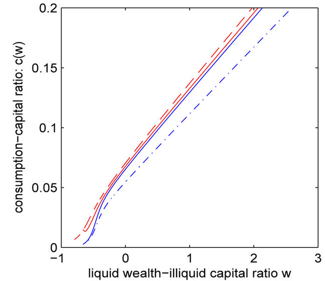 (b)
(b)
Figure 3. Market portfolio allocation-capital ratio  and consumption-capital ratio
 . All parameter values are given in Section “Quantative Results”.
consumption and portfolio allocation for the entrepreneur with sufficient cash holdings. Interestingly, we find that the need to burn cash to bring forward liquidation option exercise dominates the cash hoarding motive, thus making the boost of investment, consumption and portfolio allocation when the firm is near the liquidation boundary.
During a financial crisis, the entrepreneur cuts investment, delays consumption, lowers portfolio allocations and sometimes engages in asset sales. This is especially true when the entrepreneur enters the crisis with low cash reserves. These predictions are consistent with the stylized facts about firm behaviour during the recent financial crisis. In prospect of the possible arrival of the good state, the investment, consumption and portfolio allocation is higher than the benchmark for the entrepreneur with sufficient wealth. As the firm is near the liquidation boundary, the entrepreneur brings investment, consumption and portfolio allocation back to the benchmark to maintain the business and wait for the good state to come.
6. Acknowledgements
The authors acknowledge financial support from Natural Science Foundation of China (# 71202007), Innovation Program of Shanghai Municipal Education Commission (# 13ZS050), “Chen Guang” Project of Shanghai Municipal Education Commission and Shanghai Education Development Foundation (# 12CG44) and Innovation Research Fund of Shanghai University of Finance and Economics (# CXJJ-2013-317 and # CXJJ-2013-312)
REFERENCES
- J. Hamilton, “A New Approach to the Economic Analysis of Nonstationary Time Series and the Business Cycle,” Econometrica, Vol. 57, No. 2, 1989, pp. 357-384. doi:10.2307/1912559
- T. Honda, “Optimal Portfolio Choice for Unobservable and Regime-Switching Mean Returns,” Journal of Economic Dynamic & Control, Vol. 28, No. 1, 2003, pp. 45- 78. doi:10.1016/S0165-1889(02)00106-9
- X. Guo, J. Miao and E. Morellec, “Irreversible Investment with Regime Shifts,” Journal of Economic Theory, Vol. 122, No. 1, 2005, pp. 37-59. doi:10.1016/j.jet.2004.04.005
- M. Campello, J. R. Graham and C. R. Harvey, “The Real Effects of Financial Constraints: Evidence from a Financial Crisis,” Journal of Financial Economics, Vol. 97, No. 3, 2010, pp. 470-487. doi:10.1016/j.jfineco.2010.02.009
- V. Ivashina and D. Scharfstein, “Bank Lending during the Financial Crisis of 2008,” Journal of Financial Economics, Vol. 97, No. 1, 2010, pp. 319-338. doi:10.1016/j.jfineco.2009.12.001
- C. Wang, N. Wang and J. Yang, “A Unified Model of Entrepreneurship Dynamics,” Journal of Financial Economics, Vol. 106, No. 1, 2012, pp. 1-23. doi:10.1016/j.jfineco.2012.05.002
- E. Hurst and A. Lusardi, “Liquidity Constraints, Household Wealth, and Entrepreneurship,” Journal of Political Economy, Vol. 112, No. 2, 2004, pp. 319-347. doi:10.1086/381478
- N. Herranz, S. Krasa and A. Villamil, “Entrepreneurs, Legal Institutions and Firm Dynamics,” Unpublished Working Paper, University of Illinois, 2009.
- H. Chen, J. Miao and N. Wang, “Entrepreneurial Finance and Non-Diversifiable Risk,” Review of Financial Studies, Vol. 23, No. 12, 2010, pp. 4348-4388. doi:10.1093/rfs/hhq122
- H. E. Leland, “Corporate Debt Value, Bond Covenants, and Optimal Capital Structure,” Journal of Finance, Vol. 49, No. 4, 1994, pp. 1213-1252. doi:10.1111/j.1540-6261.1994.tb02452.x
- R. E. Hall and S. E. Woodward, “The Burden of the NonDiversifiable Risk of Entrepreneurship,” American Economic Review, Vol. 100, No. 3, 2010, pp. 1163-1194. doi:10.1257/aer.100.3.1163
- J. Driffill, T. Kenc and M. Sola, “Merton-Style Option Pricing under Regime Switching,” Working Paper, 2002.
- H. Chen, “Macroeconomic Conditions and the Puzzles of Credit Spreads and Capital Structure,” Journal of Finance, Vol. 65, No. 6, 2010, pp. 2171-2212. doi:10.1111/j.1540-6261.2010.01613.x
- P. Bolton, H. Chen and N. Wang, “Market Timing, Investment and Risk Management,” Journal of Financial Economics, in press, 2012.
- F. Hayashi, “Tobin’s Marginal q and Average q: A Neoclassical Interpretation,” Econometrica, Vol. 50, No. 1, 1982, pp. 213-224. doi:10.2307/1912538
- R. C. Merton, “Optimum Consumption and Portfolio Rules in a Continuous-Time Model,” Journal of Economic Theory, Vol. 3, No. 3, 1971, pp. 373-413. doi:10.1016/0022-0531(71)90038-X
- D. Duffie and L. G. Epstein, “Stochastic Differential Utility,” Econometrica, Vol. 60, No. 2, 1992, pp. 353-394. doi:10.2307/2951600
- J. C. Eberly, S. Rebelo and N. Vincent, “Investment and Value: A Neoclassical Benchmark,” Unpublished Working Paper, Northwestern University and HEC Montreal, 2009.
- C. A. Hennessy and T. M. Whited, “How Costly Is External Financing? Evidence from a Structural Estimation,” Journal of Finance, Vol. 62, No. 4, 2007, pp. 1705-1745. doi:10.1111/j.1540-6261.2007.01255.x
Appendix A. Details for Theorem 1
We conjecture that the value function is given by Equation (1.17). Using homogeneity property of , we can obtain Equation(1.25), (1.26) and (1.27) for
 ,
,  and
and  respectively. Substituting these results into Equation (1.13), we obtain the system of ODEs, i.e. Equations (1.18) and (1.19).
We consider the lower liquidation boundary . When
 , the entrepreneur liquidates the firm. Using the value-matching condition at
 , we have
 (1.1.1)
where  is given by
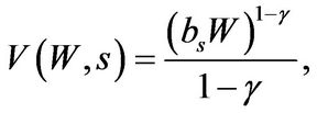 (1.1.2)
is the agent’s value function after liquidation and with no business. The entrepreneur’s optimal liquidation strategy implies the following smooth-pasting condition at the endogenously determined liquidation boundary :
:
 (1.1.3)
Using , Equations (1.1.1)-(1.1.3), and simplifying, we obtain the scaled value-matching and smooth pasting conditions given in Equations (1.23) and (1.24), respectively.
As  approaches infinity, firm value approaches the first-best value and
which implies Equation (1.22).
The CE wealth , where
  is given by
 (1.1.4)
Appendix B. Calculation of  and
and ,
,  and
and 
Let ,
,  , and replace them in Equations (1.18) and (1.19), we have
 (1.2.1)
 (1.2.2)
When w converges to infinity,  approaches to
 ,
,  approaches to
  and the coefficient before w is zero:
 (1.2.3)
 (1.2.4)
Solving Equations (1.2.3) and (1.2.4), we obtain that  and
and  satisfy
 (1.2.5)
 (1.2.6)
Consider the remaining part, and we find that  and
and  satisfy
 (1.2.7)
 (1.2.8)