Journal of Mathematical Finance
Vol.3 No.2(2013), Article ID:31818,5 pages DOI:10.4236/jmf.2013.32027
Calculating First Moments and Confidence Intervals for Generalized Stochastic Dividend Discount Models
Department of Mathematics and Computer Science, Royal Military College, Kingston, Canada
Email: hurley_w@rmc.ca
Copyright © 2013 William J. Hurley. This is an open access article distributed under the Creative Commons Attribution License, which permits unrestricted use, distribution, and reproduction in any medium, provided the original work is properly cited.
Received January 28, 2013; revised March 19, 2013; accepted April 2, 2013
Keywords: Dividend Discounting; Stochastic; Bernoulli
ABSTRACT
This paper presents models of equity valuation where future dividends are assumed to follow a generalized Bernoulli process consistent with the actual dividend payout behavior of many firms. This uncertain dividend stream induces a probability distribution of present value. We show how to calculate the first moment of this distribution using functional equations. As well, we demonstrate how to calculate a confidence interval using Monte Carlo simulation. This first moment and interval allows an analyst to determine whether a stock is overor under-valued.
1. Introduction
Dividend discount models are a common feature of most introductory finance textbooks. Normally the Gordon Growth Model [1] is one of the techniques used to illustrate the calculation of the cost of equity capital. Gordon assumes that the dividend stream will increase at a constant geometric growth rate in perpetuity. There have been variations of this model. All of them assume that future dividends will follow a fixed, mechanistic path.
These deterministic dividend streams are not really consistent with the payout policies of most firms. Typically a firm will hold a dividend constant until such time as it can see itself being able to increase it and then maintain the increase. Such dividend streams are characterized by uncertainty in that an analyst would never be certain when and by how much a dividend was going to increase. Hurley and Johnson [HJ, 2-4] have offered a series of dividend discount models consistent with these two characteristics. A good summary of these models can be found in Hurley and Fabozzi [5].
The contribution of this paper is a complete generalization of these models. I model two components of dividend uncertainty. First, in each period, the dividend is assumed to either increase or stay the same with a given probability. Second, if the dividend does increase, the increase is also modeled as a random variable. In addition, I also consider two functional forms for the dividend increase: in one, the increase is multiplicative; in the other, it is additive. For each valuation model, I show how to compute a first moment and a confidence interval. This allows an analyst to compare the current market price of the stock to this moment and interval and in so doing determine whether or not the share is overor under-valued.
2. Stochastic Dividend Discount Models
Going back to J. B. Williams [6], the value,  of a common share can be written
 (1)
(1)
where  is the dividend in period t, and k is the discount rate. Gordon [1] made the assumption that future dividends would increase at a geometric rate in perpetuity,
 (2)
(2)
and, under this assumption, value can be shown to be
 (3)
(3)
There have been variations of Gordon’s assumption. Like Gordon’s, all of them posit a future dividend stream that is known and increasing.
Table 1 shows a dividend stream for a hypothetical firm, ABC Corp. This dividend payout pattern has all the

Table 1. A sample dividend history.
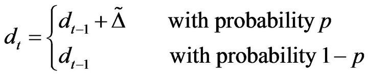
characteristics of real-world dividend streams. Note that, each period, the dividend either stays the same or increases. I model this stochastic behavior by assuming that the dividend payment in period t is given by
 (4)
(4)
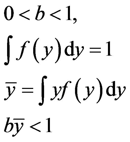
where  is a random growth rate, and p is the probability the dividend increases.
  is assumed to have a density
  and first moment
 (5)
(5)
where  I term this dividend process a Geometric Bernoulli Process (GeoBP) and denote its present value by
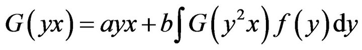
  To get its first moment,
  we need to solve the following functional equation:
 (6)
(6)
The first term on the right-hand side is the case where the dividend stays the same and the value in one period’s time,  is discounted to the present by dividing by
  The second term is the case where the dividend increases by a random amount γ. Hence the value in one period’s time is
  and this has to be discounted one period and integrated over
  to get an expected present value. Finally these two present values are weighted by 1 – p and p respectively.
In addition, I model an Additive Bernoulli Process (AddBP) where the dividend payment in period t is given by
 (7)
(7)
where  is a random additive increment in the dividend, and p is the probability the dividend increases.
  is assumed to have a density
  and first moment
  Again, I will compute a first moment for present value,
  by solving the following equation:
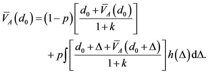 (8)
(8)
This equation has the same structure as (6) except that the dividend is additive rather than geometric. Both Equations (6) and (8) are functional equations and their solution is discussed in the next section.
Computing first moments provides a point estimate of value and this is certainly beneficial. But the more useful calculation within this modeling structure is a confidence interval for value. Effectively a confidence interval gives a band-width for value and the existing stock price (and indeed the recent history of the stock price movement) can be assessed against this interval to determine whether the share is overor under-valued. If it were true that the distributions of present value under the assumed stochastic processes were approximately normal, we could calculate the second moments,  and
and  using variations of (6) and (8), then get variances and confidence intervals. However these processes tend to give rise to distributions that are skewed and, hence, the normal distribution does not usually apply. For this reason, we resort to computing confidence intervals using a Monte Carlo procedure which we detail herein.
3. Finding First Moments
To solve the functional Equations in (6) and (8), we need the following lemmas.
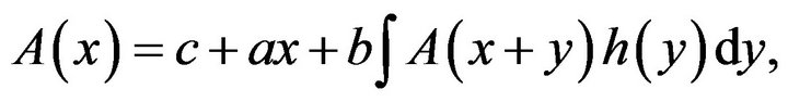
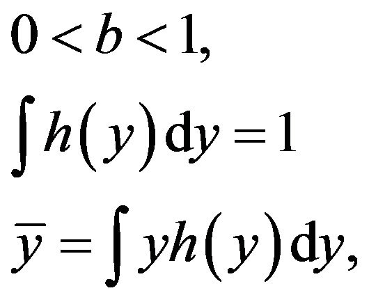
Lemma 1. The functional equation
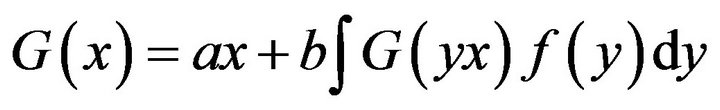 (9)
(9)
where
 (10)
(10)
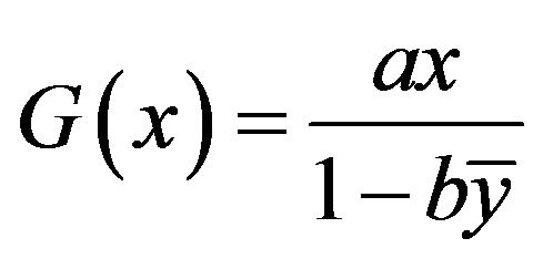
has a solution
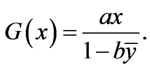 (11)
(11)
Proof. Substitute the solution in (11) into the righthand side of (9) to get:
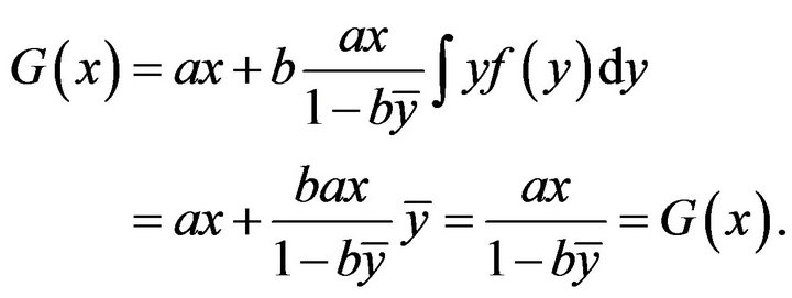 (12)
(12)
Hence (11) is solution and the proof is complete.
Showing that a functional equation has a particular solution is one thing. Calculating it is a different matter. To get the solution in (11), we begin by evaluating  in (9) at
  giving
 (13)
(13)
We then substitute result into the right-hand side of (9) for  This gives
 (14)
(14)
where  denotes expectation over
  Continuing this substitution and evaluation process
  more times yields
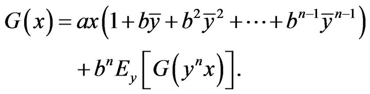 (15)
(15)
Taking the limit of the right-hand side as ![]() goes to infinity yields
goes to infinity yields
 (16)
(16)
since  as
as ![]()
Lemma 2. The functional equation
 (17)
(17)
where
 (18)
(18)
has a solution
 (19)
(19)
Proof. Substitute the solution in (19) into the righthand side of (17):
 (20)
(20)
Hence (19) is a solution of (17) and the proof is complete.
The solution in (19) can be obtained in the same way as for (11). With these lemmas, we are now in a position to get first moments.
Proposition 1. Suppose the future dividend stream follows a GeoBP. Then
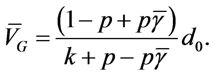 (21)
(21)
Proof. Equation (6) is equivalent to (9) when
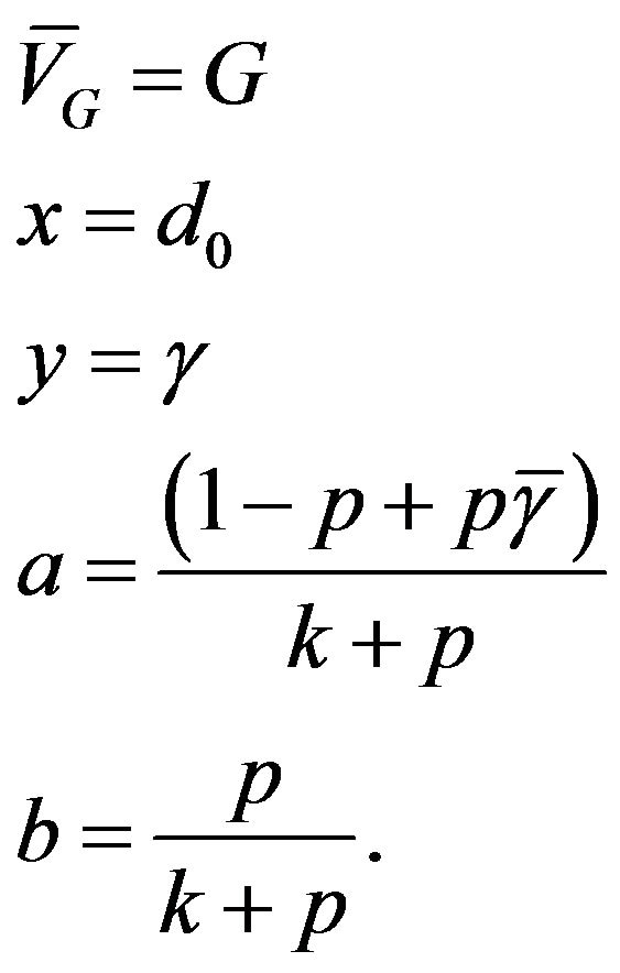 (22)
(22)
Substituting for the parameters and variables in (11) gives the required result.
This solution is related to the Gordon model in the following way. Letting  we have
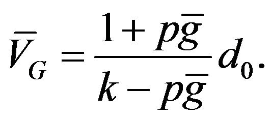 (23)
(23)
But note that  is just the expected geometric growth rate. Hence this expected value,
  is the same as the one produced by the Gordon model when the deterministic growth rate is replaced by an expected growth rate.
Equation (21) is a generalization of a number of other models. For instance, HJ [4] develop a multinomial geometric model where, each period, the dividend can change by a geometric rate with probability
  for
for  where
where  Under these assumptions, HJ show that the first moment is
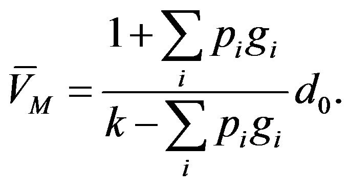 (24)
(24)
This is easily derived using the generalization above by noting that the expected growth rate is 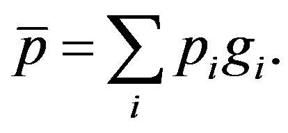
Proposition 2. Suppose the future dividend stream follows an AddBP. Then
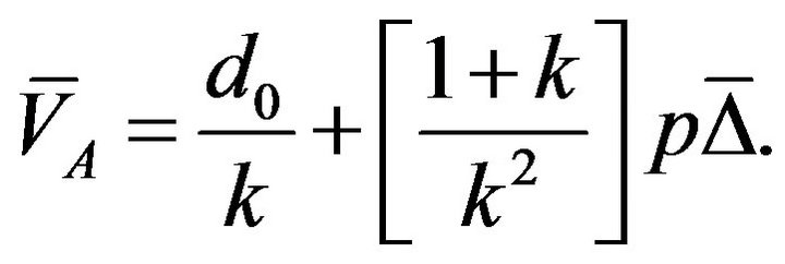 (25)
(25)
Proof. As in the proof for Proposition 1, we substitute (25) into the right-hand side of (8) and the result follows.
This expected value is the generalization of a number of other models. For instance consider Yao’s model [7]. He posits the following dividend process:
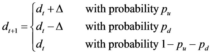 (26)
(26)
and derives the value
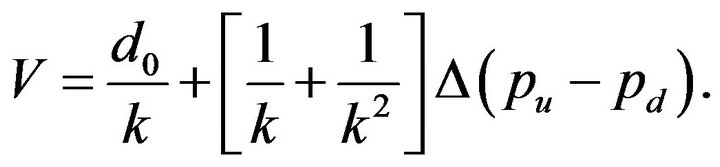 (27)
(27)
Note that this is easily derived using (25). The expected increase in the dividend is
 (28)
(28)
and
 (29)
(29)
Substituting these two into (25) yields Yao’s result.
4. Getting Confidence Intervals
In the traditional dividend discount literature, a point estimate of value is compared to a stock price to determine whether the share is overor under-valued. With stochastic dividend discount models, a share’s market price can be assessed against a confidence interval. If the present value of the dividend stream is normally distributed, it would be a simple matter to calculate the second moment (again using functional equations) and then get the desired interval. However, in practice, these distributions tend to be skewed. Hence it is best to take a Monte Carlo approach to determine an approximate confidence interval.
By way of example, suppose we calculate a 90% confidence interval for the dividend history shown in Table 1. If one looks at first differences of these dividends, they are more consistent with a geometric process than an additive. Consequently we need to estimate a value for  and the distribution of
  Over the past 16 dividend payments, the dividend increased 7 times. Therefore I estimate
 (30)
(30)
I have assumed that  is normally distributed. The sample mean and standard deviation serve as estimates of the normal distribution parameters:
 (31)
(31)
In addition I assume that  and
and 
A Monte Carlo simulation is easily executed in EXCEL using @RISK. I calculated the present value of future dividends using only the first 100 periods (periods 101 and beyond are truncated). A histogram for 10,000 iterations of present value is shown in Figure 1. First note that the distribution is skewed to the right. Second,
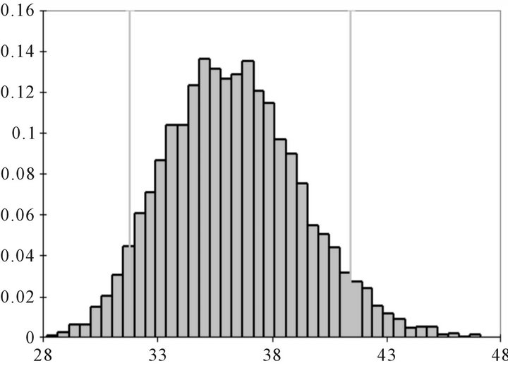
Figure 1. Histogram of the distribution of present value.
the simulation produces a mean of $36.32, which is very close to the value produced by (21):
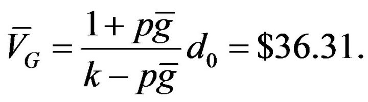 (32)
(32)
The 90% confidence interval, [$31.79, $41.43], is estimated from the @RISK output. So if the stock were trading at $25.75, we might conclude it was under-valued; if it were trading at $40.25, we might conclude it to be over-valued.
5. Summary
In this paper, I have presented two generalized stochastic dividend discount models. One assumes that dividend growth is geometric; the other assumes it is additive. I derive expressions for expected present value and show how to use Monte Carlo simulation to produce a confidence interval for this value. This confidence interval allows an analyst to better determine whether a share is overor under-valued.
REFERENCES
- M. J. Gordon, “The Investment, Financing and Valuation of the Corporation,” Irwin, Homewood, Illinois, 1952.
- W. J. Hurley and L. D. Johnson, “A Realistic Dividend Valuation Model,” Financial Analysts Journal, Vol. 50, No. 4, 1994, pp. 50-54. doi:10.2469/faj.v50.n4.50
- W. J. Hurley and L. D. Johnson, “Stochastic Two-Phase Dividend Discount Models,” Journal of Portfolio Management, Vol. 23, No. 4, 1997, pp. 91-98. doi:10.3905/jpm.1997.409614
- W. J. Hurley and L. D. Johnson, “Generalized Markov Dividend Discount Models,” The Journal of Portfolio Management, Vol. 25, No. 1, 1998, pp. 27-31. doi:10.3905/jpm.1998.409658
- W. J. Hurley and Frank Fabozzi, “Dividend Discount Models,” In: F. J. Fabozzi, Ed., Selected Topics in Equity Portfolio Management, New Hope, Pennsylvania, 1998.
- J. B. Williams, “The Theory of Investment Value,” Harvard University Press, Cambridge, 1938.
- Y. L. Yao, “A Trinomial Dividend Valuation Model,” Journal of Portfolio Management, Vol. 23, No. 4, 1997, pp. 99-103. doi:10.3905/jpm.1997.409618