ABSTRACT

In this paper, we present the fundamental framework of the evaluation problem under which the evaluation operator satisfying some axioms is linear. Based on the dynamic linear evaluation mechanism of contingent claims, studying this evaluation rule in the market driven by fractional Brownian motions has led to a dynamic capital asset pricing model. It is deduced here mainly with the fractional Girsanov theorem and the Clark-Haussmann-Ocone theorem.

1. Introduction

In the 1960s, Sharpe (1964), Lintner (1965) and Mossin (1966) established the famous Capital Asset Pricing Model (CAPM for short). The CAPM has been used and cited in the literature over the past several decades. Some efforts have been made to extend this model. Dybvig and Ingersoll [1] investigated the relationship between the linear evaluation rule and the CAPM. They proved that the standard mean-variance separation theorem obtained in a complete market only if all investors had quadratic utility. In addition, the familiar CAPM pricing relation could hold for all assets in a complete market only if arbitrage opportunities existed. A description of the relationship between the linear evaluation rule and the theory of Markowitz portfolio choice can be found in [2], which they derived a general representation for asset prices that displayed the role of conditioning information. This representation was then used to examine restrictions implied by asset pricing models on the unconditional moments of asset payoffs and prices. An exhaustive discussion of the equivalence of these three theories (the linear evaluation rule, the CAPM and the theory of Markowitz portfolio choice) was presented in [3]. Shi [4] gave a fundamental probability model in the two-period security market. Under some conditions, if the linear evaluation rule holds, then there would be a stochastic discount factor. If this is true, all three theories (CAPM, linear evaluation rule and Markowitz portfolio choice) are equivalent. They are mainly deduced by the method of Hilbert space and stochastic discount factor. Particularly, CAPM could be deduced from the linear evaluation rule in the intertemporal market.

Since nowadays the market fluctuates promptly and dealings in securities require extremely high speed, no discrete-time model could adapt to the market well. However, the continuous-time model is regarded as a good approximation to real scenarios. If we assume that the model is continuous, then it facilitates the use of stochastic differential equations, stochastic analysis, and so on, to obtain some profound and concise conclusions. The famous Black-Scholes option pricing model is a classic issue of continuous-time finance. The fundamental theorem of asset pricing, the portfolio choice of securities and the CAPM all have their continuous-time version. Zhou and Wu [5] deduced the dynamic CAPM from the dynamic linear evaluation rule in the market driven by the Levy processes. They mainly used the predictable representation property in weak form and the Girsanov theorem of the Levy processes to obtain the results.

Ever since the pioneering work of Hurst [6,7] and Mandelbrot [8], the fractional Brownian motion has played an increasingly important role in various fields such as hydrology, economics, and telecommunications [9-12]. In this paper, we study the dynamic CAPM in the fractional Brownian motion environment, which represents a new perspective.

The remaining sections of this article are organized as follows: Some preliminaries of fractional Brownian motion are presented in Section 2. Section 3 presents the fundamental framework of the evaluation problem under which the evaluation operator satisfying some axioms is linear. In Section 4, we investigate the relationship between the dynamic linear evaluation rule and the dynamic CAPM in the market driven by fractional Brownian motions. Section 5 provides the conclusions.

2. Preliminaries of Fractional Brownian Motion

As preparation, collecting some important results concerning fractional Brownian motion is essential in this section. Also, it is necessary to introduce notation for further use.

Recall that if 0 < H < 1, then the fractional Brownian motion with Hurst parameter H is a Gaussian process with mean

and covariance

where and denotes the expectation with respect to the probability law for Assume thatis defined on the of subsets of generated by the random variables. For simplicity we assume

If, then coincides with the standard Brownian motion, which has independent increments. If then has a long-range dependence, in the sense that if we put:

then.

For any the process is self-similar in the sense that has the same law as for any See [8,12] for more information about fractional Brownian motion.

Due to these properties, with Hurst parameter has been suggested as a useful tool in many applications [11], including finance.

Fix a Hurst constant, Since H is fixedthe probability measure is denoted by P and the filtration is denoted by. In this case we have the integral representation [13] and the references therein):

where is a standard Brownian motion (Wiener process) and

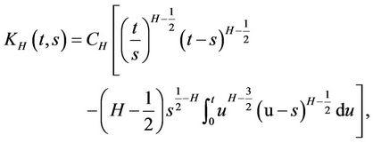
with being a constant such that

With this we associate an operator

Recently, stochastic calculus for fractional Brownian motion has been developed by many researchers [13,14].

2.1. Quasi-Conditional Expectation and Fractional Girsanov Theorem

The quasi-conditional expectation is important to obtain the main results. It was initially introduced to find the hedging strategy in an application to finance [9]. Let f and g be two continuous functions on [0, T], where is a fixed time horizon. Define

where

when, denote:

Apparently, for any is a Hilbert scalar product. Let be the completion of the continuous functions under this Hilbert norm. The elements in may be distributions [15].

For any let denote the set of all real symmetric functions variables on such that

It is known [15] that is a subspace of and they are not identical. Let denote the set of such that F has the following chaos expansion:

where when restricted to is in for alland

is the multiple stochastic integral (for the multiple integrals and the chaos expansion, [14,16].

Definition 2.1 If then the quasiconditional expectation [7] is defined as

where

The following Lemma 2.1 (resp. Lemma 2.2) is from [17] Theorem 3.9 (resp. Theorem 3.11).

Lemma 2.1 Let be continuous such that is an increasing function. Denote where g is a measurable real valued function of polynomial growth and Then

The following lemma is an analogue of the StriebelKallianpur formula. It is called a form of fractional Girsanov theorem.

Lemma 2.2 Let and be continuous functions of s in [0, T] and

Consider the translation of

Let Q denote the probability measure given by

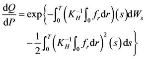
Then is a fractional Brownian motion under Q. If satisfies the integral equation

then for any measurable function g of exponential growth,

where

The above two lemmas are indispensable to the main results.

2.2. A fractional Clark-Haussmann-Ocone (CHO) Theorem

Finally let us review a fractional version of the ClarkHaussmann-Ocone (CHO) representation obtained in Theorem 4.5 in [9].

Lemma 2.3 Let be -measurable, then exists. Define

Here is the stochastic gradient (Malliavin derivative) of G at t. Then,

Refer to Section 4 in [9] for details.

3. Mechanism of Evaluation of Contingent Claims

The mathematical formulation to the evaluation problem is provided below.

Let be a complete probability space defined in Section 2, and a filtration satisfying the usual conditions, Fix a time interval and set

For all define the inner product of these two random variables Then is a Hilbert space, which denotes the subspace of all contingent claims. is the space of -measurable and square-integrable random variables.

For all contingent claims, denote the evaluated value by

At each time t,

is an evaluation operator. We will present the following axiomatic hypotheses of the evaluation operator:

(H1)

(H2)

The following lemma is from [5] Lemma 2.1.

Lemma 3.1 For hypotheses (H1) and (H2) hold if and only if it is a continuous linear function defined on

(H3) For each if , then , if in addition then.

Remark 3.1 The financial meaning of hypothesis (H1) is self evident. Hypothesis (H3) is similar to that there is no arbitrage in the market. Hypotheses (H1)-(H3) are the static properties of the linear evaluation operator.

Remark 3.2 From Lemma 3.1, we know that is a continuous linear function defined on the Hilbert space. It then follows from (H3) and the Riesz representative theorem that: there exists , such that

Since, by [16] Theorem 3.1 and 3.2, without loss of generality, we may assume that there exists a Borel measurable (deterministic) function such that

(H4) For each,

(3.1)

Remark 3.3 Hypothesis (H4) is the dynamic characteristic of the linear evaluation rules, which is shown uniquely in this paper. For the financial meaning of equation 3.1, you may see [5] Remark 2.2.

Now comes the explicit form of this evaluation operator in the market driven by fractional Brownian motion.

4. Deduce the Dynamic CAPM from the Dynamic Linear Evaluation Rule

4.1. The Explicit Form of the Evaluation Operator

Theorem 4.1 Let be continuous such that is an increasing function. Denote where g is measurable real valued function of polynomial growth such that If there exists a continuous function satisfying the integral equation

then let Q denote the probability measure given by

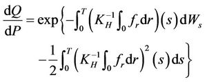
We have

(4.1)

where

Here is the stochastic gradient (Malliavin derivative) of G at s.

Proof. Let be continuous function such that is an increasing function. Denote where g is measurable real valued function of polynomial growth such that By Lemma 2.2, we know that if there exists a continuous function satisfying the integral equation

then consider the translation of

Let Q denote the probability measure given by

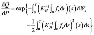
Then is a fractional Brownian motion under Q. It follows from (3.1) and Lemma 2.2 that

Let. Define

where is the stochastic gradient (Malliavin derivative) of G at s. By Lemma 2.1 and 2.3, we obtain that

Thus,

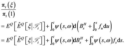
The theorem is proved.

Suppose that Remark Equation (4.1) can be formally expressed as

(4.2)

4.2. Deduce the Dynamic CAPM from the Dynamic Linear Evaluation Rule

In fact, the CAPM attempts to relate the one-period rate of return of a specified security i, to the oneperiod rate of return of the entire market (as measured, say, by the Standard and Poor’s index of 500 stocks). If is the risk-free interest rate (usually taken to be the current rate of a US Treasury bill) then the model assumes that, for some constant

where is a normal random variable with mean 0 that s values of

the CAPM model (which treats as a constant) implies that

or, equivalently, that where

That is, the difference between the expected rate of return of the security and the risk-free interest rate is assumed to equal times the difference between the expected rate of return of the market and the risk-free interest rate.

From the above formula, we know that the rate of return of a single security is determined by the relationship between this single security and the market portfolio.

Assume that the non-risk interest rate is 0. Equation (4.2) indicates that the instantaneous return of the contingent claim can be decomposed into two parts. Containing fractional Brownian motion, the first term to the right side denotes the stochastic volatility and denotes the volatility rate. The volatility rate changes in compliance with the change of the contingent claim. In the other term, f is determined by the evaluation operator itself and it reflects the mechanism of the market. reflects the extent to which the instantaneous return of the contingent claim and the return of the market portfolio are related. Therefore, the instantaneous return of the contingent claim is mainly determined by this dependence. Equation (4.2) can be regarded as another version of CAPM. Accordingly, Equation (4.2) indicates that the instantaneous return of the contingent claim is mainly determined by the extent to which the instantaneous return of the contingent claim and the return of the market portfolio are related.

From the discussion above, we deduce the dynamic CAPM from the dynamic linear evaluation rule in the market driven by fractional Brownian motion.

5. Conclusion

In this paper, we first give some preliminaries of fractional Brownian motion. Then, we present the fundamental framework of the evaluation problem under which the evaluation operator satisfying some axioms is linear. Based on the dynamic linear evaluation mechanism of contingent claims, studying this evaluation rule in the market driven by fractional Brownian motions has led to a dynamic capital asset pricing model. It is deduced here mainly with the fractional Girsanov theorem and the Clark-Haussmann-Ocone theorem.

6. Acknowledgements

The authors would like to thank the referees for the careful reading of the paper and helpful suggestions. Part of this work was completed when author Zhou was visiting the University of Kansas. We would like to thank Professor Yaozhong Hu and David Nualart, and Dr. Alexander Uhl for their help.

REFERENCES

NOTES

^*This research is supported by the Natural Science Foundation of China under grants 11001029 and 10971220, the Fundamental Research Funds for the Central Universities (BUPT2012RC0709).

REFERENCES

- P. H. Dybvig and J. E. Ingersoll, “Mean-Variance Theory in Complete Markets,” Journal of Business, Vol. 55, No. 2, 1982, pp. 233-251. doi:10.1086/296162
- L. P. Hansen and S. F. Richard, “The Role of Conditioning Information in Deducing Testable Restrictions Implied by Dynamic Asset Pricing Models,” Econometrica, Vol. 55, No. 3, 1987, pp. 587-614. doi:10.2307/1913601
- J. H. Cochrane, “Asset Pricing,” Princeton University Press, Princeton, 2001.
- S. Z. Shi, “Ten Presentations of Financial Econometrics,” Shanghai Dometic Publishing, Shanghai, 2004.
- Q. Zhou and W. X. Wu, “From Dynamic Linear Evaluation Rule to Dynamic Capital Asset Pricing Model,” System EngineeringTheory and Practice, Vol. 27, No. 5, 2007, pp. 48-54. doi:10.1016/S1874-8651(08)60033-2
- H. E. Hurst, “Long-Term Storage Capacity in Reservoirs,” Transactions of the American Society of Civil Engineers, Vol. 55, 1951, pp. 400-410.
- H. E. Hurst, “Methods of Using Long-Term Storage in Reservoirs,” Proceedings of the Institution of Civil Engineers Part 1, Vol. 5, 1956, pp. 519-590.
- B. B. Mandelbrot and J. W. Van Ness, “Fractional Brownian Motions, Fractional Noises and Applications,” SIAM Review, Vol. 10, No. 4, 1968, pp. 422-437. doi:10.1137/1010093
- Y. Hu and B. Øksendal, “Fractional White Noise Calculus and Applications to Finance, Infinite Dimensional Analysis,” Quantum Probability and Related Topics, Vol. 6, No. 1, 2003, pp. 1-32.
- Y. Hu, B. Øksendal and A. Sulem, “Optimal Consumption and Portfolio in a Black-Scholes Market Driven by Fractional Brownian Motion,” Infinite Dimensional Analysis, Quantum Probability and Related Topics, Vol. 6, No. 4, 2003, pp. 519-536. doi:10.1142/S0219025703001432
- B. B. Mandelbrot, “Fractals and Scaling in Finance: Discontinuity, Concentration, Risk,” Springer & Verlag, Berlin, 1997.
- A. Shiryaev, “On Arbitrage and Replication for Fractal Models,” In: A. Shiryaev and A. Sulem, Eds., Workshop on Mathematical Finance, INRIA, Paris, 1998.
- Y. Hu, “Integral Transformations and Anticipative Calculus for Fractional Brownian Motions,” American Mathematical Society, Providence, 2005.
- F. Biagini, Y. Hu, B. Øksendal and T. S. Zhang, “Stochastic Calculus for Fractional Brownian Motion and Applications,” Springer, London, 2008. doi:10.1007/978-1-84628-797-8
- V. Pipiras and M. S. Taqqu, “Integration Questions Related to Fractional Brownian Motion,” Probability Theory and Related Fields, Vol. 118, 2000, pp. 251-291. doi:10.1007/s440-000-8016-7
- T. E. Duncan, Y. Hu and B. Pasik-Duncan, “Stochastic Calculus for Fractional Brownian Motion,” SIAM Journal on Control and Optimization, Vol. 38, No. 2, 2000, pp. 582-612. doi:10.1137/S036301299834171X
- Y. Hu and S. Peng, “Backward Stochastic Differential Equations Driven by Fractional Brownian Motion,” SIAM Journal on Control and Optimization, Vol. 48, No. 3, 2009, pp. 1675-1700. doi:10.1137/070709451