ABSTRACT

In this paper, we relax the assumption of a known time horizon in optimal control models.

1. Introduction

The literature on control and optimization mainly considered a known predetermined time horizon or infinite horizon. However, the previous studies did not examine the possibility of unknown (random) time horizon. Examples include Alghalith (2009) [1], Fleming (2004) [2], and Focardi and Fabozzi (2004) [3], among many others. In some cases, it is more realistic to assume that the horizon depends on some of the stochastic factors of the model and therefore it is random. Hence, it cannot be predetermined at the initial time. For example, the horizon of the investor might depend on the stochastic asset price or any other economic factor. Therefore the investor adjusts the horizon accordingly. Consequently, the assumption of a non-random horizon is somewhat restrictive.

In this paper, we relax the assumption of a known time horizon without significantly complicating the optimal solutions. As an example, we apply our methods to a stochastic factor incomplete markets investment model. In so doing, we provide solutions for the optimal portfolio under the assumption that the investor does not have a predetermined time horizon.

2. The Model

We consider an investment model, which includes a risky asset, a risk-free asset and a random external economic factor. We use a three-dimensional standard Brownian motion based on the probability space where is the augmentation of filtration. The risk-free asset price process is

where is the rate of return and is the stochastic economic factor.

The dynamics of the risky asset price are given by

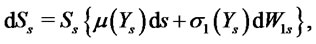(1)

where and are the rate of return and the volatility, respectively. The economic factor process dynamics are given by

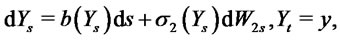(2)

and.

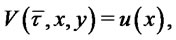
The stochastic terminal time is denoted by and its dynamics are given by

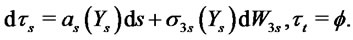
We define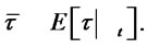

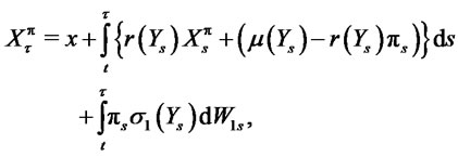
The wealth process is given by

(3)

where is the initial wealth, is the portfolio process with 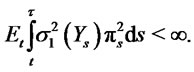The trading strategy is admissible.

The investor’s objective is to maximize the expected utility of the terminal wealth

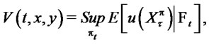(4)

where is the value function, is a continuous, bounded and strictly concave utility function.

The value function satisfies the Hamilton-JacobiBellman PDE

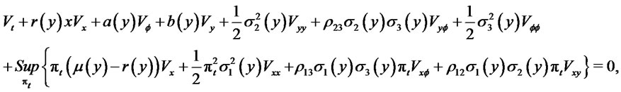
(5)

where is the correlation coefficient between the Brownian motions. Hence, the optimal solution is

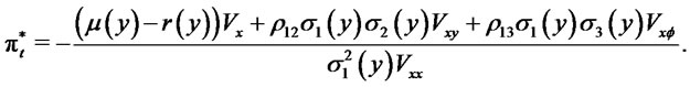(6)

Clearly, following previous studies, we can obtain an explicit solution for specific functional forms of the utility such as an exponential utility function.

REFERENCES

- M. Alghalith, “A New Stochastic Factor Model: General Explicit Solutions,” Applied Mathematics Letters, Vol. 22, No. 12, 2009, pp. 1852-1854. doi:10.1016/j.aml.2009.07.011
- W. Fleming, “Some Optimal Investment, Production and Consumption Models,” Contemporary Mathematics, Vol. 351, 2004, pp. 115-124.
- F. Focardi and F. Fabozzi, “The Mathematics of Financial Modeling and Investment Management,” Wiley, New York, 2004.