Open Journal of Safety Science and Technology
Vol.2 No.3(2012), Article ID:22588,4 pages DOI:10.4236/ojsst.2012.23013
Outbreak Detection of Spatio-Temporally Smoothed Crashes
CSIRO Mathematics, Informatics and Statistics, Sydney, Australia
Email: Ross.Sparks@csiro.au
Received May 1, 2012; revised June 10, 2012; accepted June 24, 2012
Keywords: Average Run Length; Exponential Weighted Moving Averages; Monitoring; Spatial Outbreaks; Spatio-Temporal Smoothing; Crash Outbreaks
ABSTRACT
Spatio-temporal surveillance methods for detecting outbreaks are common with the SCAN statistic setting the benchmark. If the shape and size of the outbreaks are known, then the SCAN statistic can be trained to efficiently detect these, however this is seldom the case. Therefore devising a plan that is efficient at detecting a range of outbreaks that vary in size and shape is important in practical applications. So this paper introduces a method called EWMA Surveillance Trees that uses a binary recursive partitioning approach to locate and detect outbreaks. This approach is explained and then its performance is compared to that of the SCAN statistic in a series of simulation studies. While the SCAN statistic is shown to remain the most effective at detecting outbreaks of a known shape and size, the EWMA Surveillance Trees are shown to be more robust. The method is also applied to an example of actual data from motor vehicle crashes in an area of Sydney Australia from 2000 to 2004 in order to detect dates and geographic regions with outbreaks of crashes above the expected.
1. Introduction
The SCAN statistic [1] has been successful at prospectively detecting space-time clusters. Kulldorff [2-4] has developed SCAN plans and implemented them in the SATSCAN software package for a variety of problems including Bernoulli data, Poisson counts and a spacetime permutation model using only case data, amongst others. However there are some important limitations to this approach which will be addressed in this paper. Firstly, the space-time permutation model compares incidences to what is expected under the assumption that all cases were independent of each other. That is, the expected values are determined under the assumption that there is no space-time interaction. Secondly, the spatio-temporal SCAN statistic has been criticised by Woodall et al. [5] and Han et al. [6] for not being as efficient as the CUSUM [7,8] for outbreak detection. Lastly, the ability to detect outbreaks most effectively is dependent on the choice of shape and size of the scanning window.
However, the attractiveness of the SCAN technology is that it is easy to understand, and therefore people use it. For this reason, the SCAN statistic is implemented in this paper as a benchmark for comparison. In our implementation, we considered the two dimensional scan statistic used for detecting spatial clusters as discussed in detail in the book by Glaz et al. [9]. To extend the method to the detection of three-dimensional spatio-temporal clusters, we use the lattice structure as outlined in Glaz et al. [9] and then search over this structure for groups of rectangular blocks of space and time in order to alarm for unusually high counts. The counts within the rectangular blocks of space-time are compared to their respective expected counts to measure their unusualness. Boundaries of all significant geographical regions are outlined on a map to indicate the geography of the outbreak.
The EWMA Surveillance Tree plan that is proposed in this paper addresses all of the concerns raised above. This plan also makes use of the fixed lattice structure since this structure is well suited to the application of Exponentially Weighted Moving Average (EWMA) temporal smoothing of the counts. This smoothing improves early detection over the moving average approach suggested by Kulldorff and others. Therefore this EWMA smoothing avoids the criticisms by Woodall et al. (2008) and Han et al. (2008). Also, in this paper, we compare incidences to historical expected values where the expected values can be space-time dependent. Therefore clustered outbreaks are signaled in this paper when the counts are higher than expected in a random local region. Lastly, by doing away with the scanning window all together we have removed the need for this parameterisation.
Therefore the principal goal of this paper is to compare our proposed recursive partitioning plan to the single window size SCAN statistic. Section 2 of the paper introduces the single window SCAN statistic. Section 3 describes both the EWMA smoothing process and the recursive partitioning approach that make up the EWMA Surveillance Tree plan. Section 4 provides a simulation study for comparing plans under a number of different outbreak scenarios where Average Run Length (ARL) is used to assess and compare the detection properties of plans. Section 5 describes an extension of the plan to the non-homogeneous situation. Lastly, Section 6 briefly covers an example of outbreak detection in motor vehicle crash data.
2. The SCAN Statistic
The SCAN statistic is a spatio-temporal moving average plan that looks at the number of observations in a prism of spatio-temporal space, where the height of the prism is a time window. In this paper we scan an exhaustive set of rectangular blocks (e.g., see Figure 1). This is an extension of the lattice approach described in Glaz et al. [9] to three dimensions. Kulldorff’s SCAN statistic places no restriction on the scanned space other than window size. Kulldorff’s spatial SCAN statistic thus offers more flexibility than Glaz et al. [9] spatial scans by scanning 3 dimensional space-time. This is better in terms of defining the boundary of the outbreak. However, this flexibility increases the number of tests which may reduce effectiveness of the plan.
The depth of the scanned “block” (z-axis) represents the time window over which incidents are aggregated (see Figure 1). This depth is taken as days in this paper. The union of all rectangular blocks in Figure 1 exhausts the 3-dimensional target space of interest, and will be referred to as the target block from now on. Space-time blocks are scanned for detecting outbreaks by comparing their block counts to their respective expected counts. The scanned blocks are not taken to have a fixed volume, but are constructed so that the marginal total across each row/column spatial dimension of the target block has approximately the same expected number of counts. Ideally the design is to have all small blocks with roughly the same expected values; however this is difficult in practice. Blocks are therefore constructed so that the marginal row/column totals have the same respective expected values. This design should control for variations in population sizes.
Let the daily number of crashes in the cell at the ith row, jth column and at day t be recorded as random variable  for a target block of total size A × B. Let their respective expected values be denoted by
 . The SCAN plan examines departures
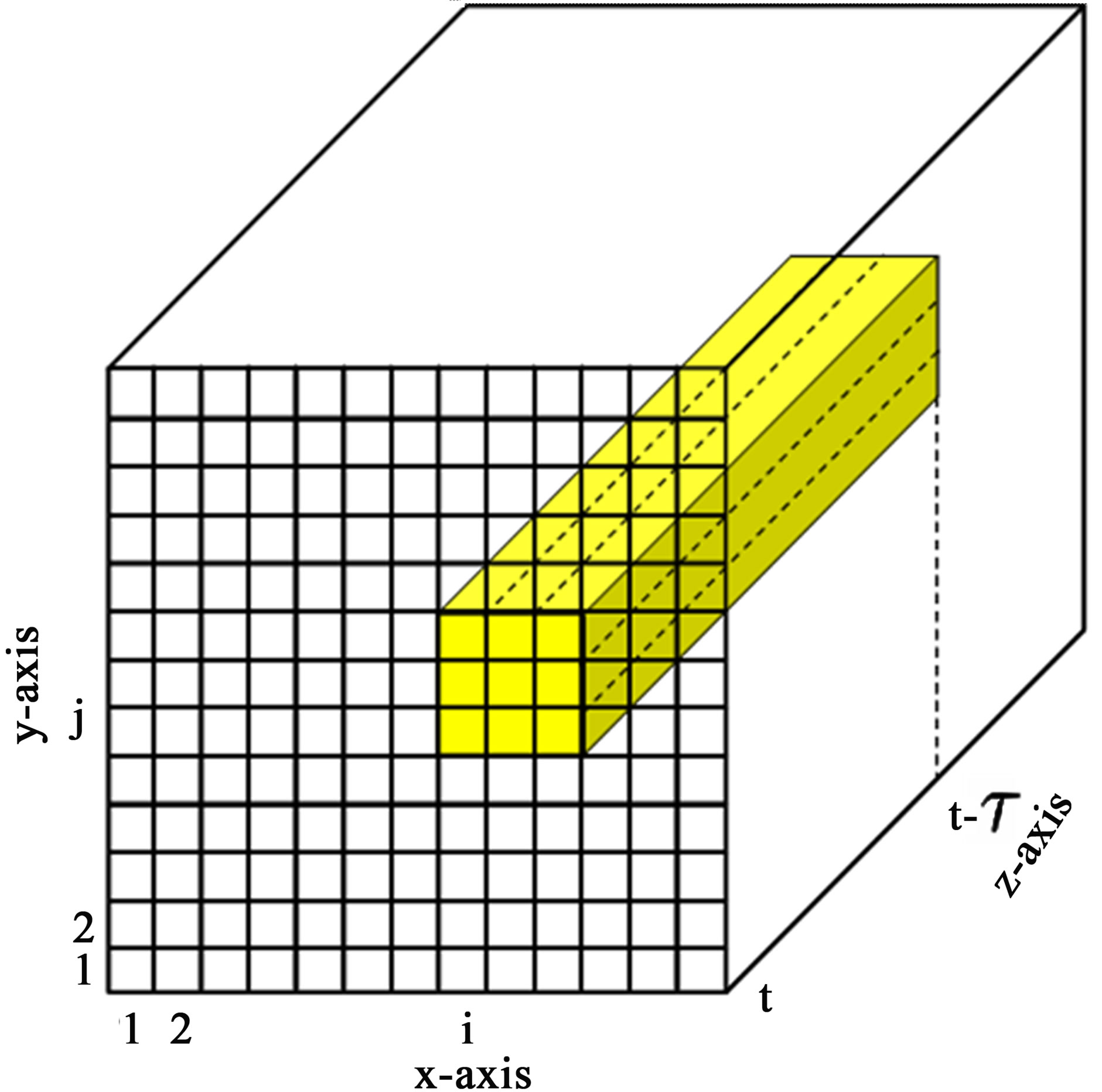
Figure 1. The mutually exclusive and exhaustive rectangular blocks in the target spatio-temporal scanning area (depth = time window). The shaded area represents the
3 × 3 × rectangular block with starting cell (i, j, t).
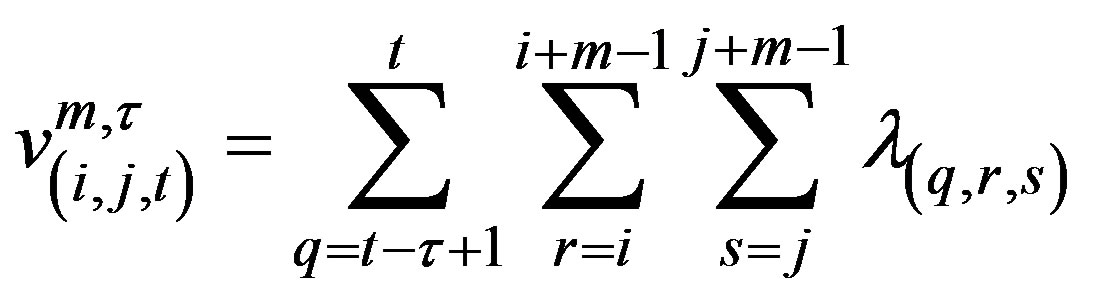
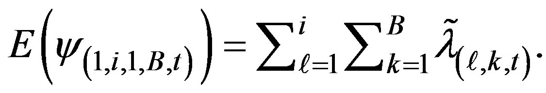
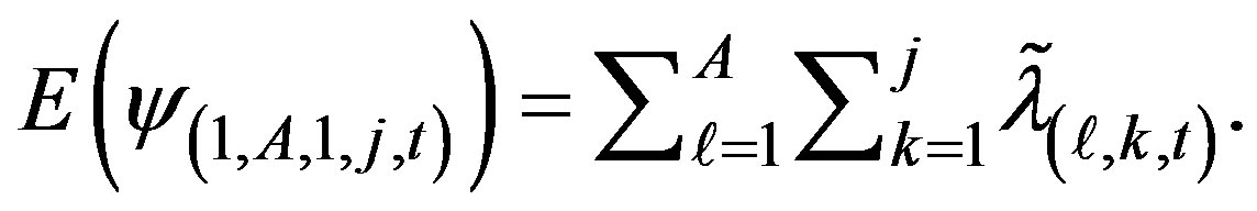
of counts from their expected values. Define total cases in a scanned spatio-temporal window of  size with starting cell (i, j, t) by
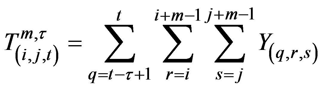 (1)
(1)
with expected values
 (2)
(2)
where 
Now  counts within a rectangular block of
  for the past
  days are assumed to be Poisson distributed with mean
 . This allows Poisson tables to be used to test whether the
  counts are significantly higher than their respective expected value
 .
.
Since we are testing many of these blocks simultaneously, we need to adjust the level of significance for this multiple testing. Bonferroni adjustments would be too conservative since overlapping blocks are examined in the exhaustive search. So instead, the threshold of the SCAN plan is based on
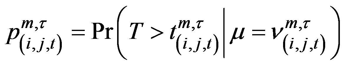
where  is the observed count on day t. A signal is given whenever
for at least one  The value of
  is a threshold designed to give a fixed false alarm rate or in-control ARL. Starting values for
  can be found by first aggregating over time and then using the method proposed by Chen and Glaz [10]. Simulation is then used to refine this threshold to deliver the appropriate threshold value.
This SCAN plan is applied in this paper with the following parameters:
• A target block with A = 100, B = 100 (using percentiles to design the lattice).
•  , the depth of window in time is taken as 10.
• m, the width and height of the window, is taken as 21.
3. EWMA Surveillance Trees
The method proposed here for comparison against the SCAN plan consists of three major steps:
1) EWMA based smoothing of observed and expected counts, first temporally then spatially;
2) Growing a surveillance tree of departures from expected value in the spatio-temporally smoothed counts using a binary recursive partitioning approach;
3) Pruning the surveillance tree to reveal outbreaks.
Each of these steps will be outlined in Sections 3.1, 3.2 and 3.3 respectively.
3.1. EWMA Smoothing
The SCAN plan examines total block counts in a moving time window of  days. This gives counts of each day in the window equal weight, independent of how close these points are from the current time point t. Define A by B matrices
  and
and , then an alternative plan is to examine an exponentially weighted moving average of the counts using
( ) and similarly smooth the expected values of these counts using

where  , and
, and  is a constant that determines how much memory to retain in the average. Larger values of
  retain less temporal memory.
Let  be the matrix of EWMA temporal smoothed counts and
  be the matrix of EWMA temporal smoothed expected values. In order to smooth the counts spatially, define a row and column smoothing matrix A with ith row and jth column elements
  for
for  where
where . Let the row totals of matrix A be
  where
where  a column vector of B ones. Let
  be a diagonal matrix with diagonal elements equal to
 , then the spatially smoothed counts are given by

and the spatially smoothed expect values are given by
The smoothing above is carried out for the rows and then the columns. This is different to smoothing using a kernel smoother that exploits distances between cells. If all cells were of equal dimensions this smoothing would be similar to the kernel smoothing with the double exponential distribution as the smoothing function. The EWMA spatial smoothing as applied in this paper has the advantages of computational simplicity and efficiency, and therefore reduces the effort needed in the simulation studies.
3.2. Growing the Surveillance Trees
Surveillance trees generate offspring by recursively partitioning either longitudinal cells or latitudinal cells into rectangular regions. The process begins with the whole target area and the focus for each partition is to find a region with unusually high smoothed counts. The term unusually high is used here to mean that the counts are significantly higher than the smoothed expected values in a statistical sense. Each partition of a parent region thus results in two offspring, one of which has the unusually high smoothed count and the other which is simply the remainder of the parent region. Each generation of offspring is grown in the same way until the smoothed counts in a parent region are not large enough to support new offspring with unusually high smoothed counts (a region with no offspring is called a terminal region). This subdivision gives rise to a representation of the target area by means of a tree data structure referred to as a Surveillance Tree.
Once partitioning has stopped for all terminal regions, then recursive pruning of the terminal nodes commences. This pruning process is outlined in the following section. Here, however, we define the steps for growing a Surveillance Tree in more detail.
In order to begin the partitioning procedure, we first need a measure of how far the smoothed count departs from the expected. Let
where  is
is  th row and
  the column the element of matrix
 , then a simple measure of departure from expected is
which is based on a transformation of Poisson counts to the normal distribution. This transformation does not adjust for changing variance due to the spatio-temporal smoothing of counts. In other words,  , but the variance of
  is not one. Howeveroverlooking the changing variance means that this measure is simple to compute.
Let the xand y-coordinates of the lattice grid lines be given by  and
and , respectively. The recursive partitioning process for finding outbreaks involves the following steps:
1) Sum smoothed counts  over all cells with xcoordinates less than or equal to
  for
for , i.e., find
Calculate expected values
2) Sum smoothed counts  over all cell with ycoordinates less than or equal to
  for
for i.e., find

Find expected values
3) Calculate  which has a constant variance for all cells means and fixed smoothing constants. Then the first offspring are established using the following steps:
a) Find the i which maximizes
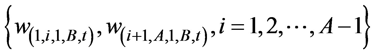
This is the best row partition.
b) Find the j which maximizes
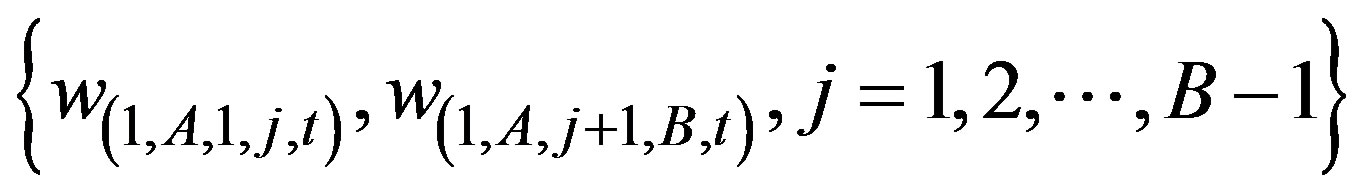
This is the best column partition.
c) Find the offspring pair which corresponds to the maximum of
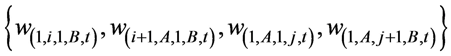 .
.
That is, if either  or
or  is the maximum, then partition the geography by splitting the space into two offspring defined by rows 1 to i and i + 1 to A in the lattice, or partition by splitting the space into two offspring by partitioning the columns into regions involving the column cells 1 to j and j + 1 to B, respectively.
4) Now repeat the process for the next generation of offspring. That is, repeat steps 1 - 3 while considering each of the two offspring generated by the first partition as parent regions in their own right.
5) The process is repeated for each new generation until either a) the counts are too low for producing any “future” generation that could be significantly higher than expected or b) that no other partitions are possible because the parent is a single cell in the lattice.
Stopping rules for recursive partitioning will be discussed later after we have dealt with the pruning process. As an example of an application with A = B = 100, Figure 2 presents the location of crashes under expected situations in the left-hand plot, and the location of crashes for an outbreak scenario in the right-hand plot. Two separate geographical clustered outbreaks were generated in the right-hand plot of Figure 2—the first in cells given by rows 1 to 11 and columns 1 to 11 and the second in cells given by rows 65 to 75 and columns 25 to 35. These are visually fairly obvious outbreaks. In Figure 3, each generation of the partitioning process for this example is presented, going up to a maximum of 4 generations. Generated outbreaks are assumed hidden when applying the recursive partitioning. For each generation, the total number of offspring doubles if there is no stopping early; each partition tries to find the best split to identify the hidden outbreaks. Note that it would take five generations to completely define all outbreaks in Figure 3. By this stage most offspring have too few observations in them to warrant further partitioning, however some generations may progress to the 6th generation
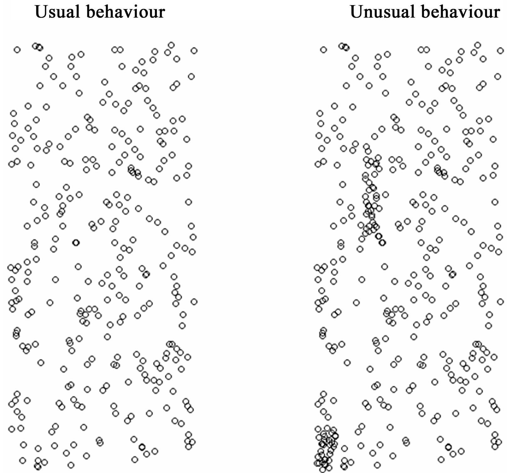
Figure 2. Plots of incident location—left plot indicating usual incidents and right plot unusual behaviour.
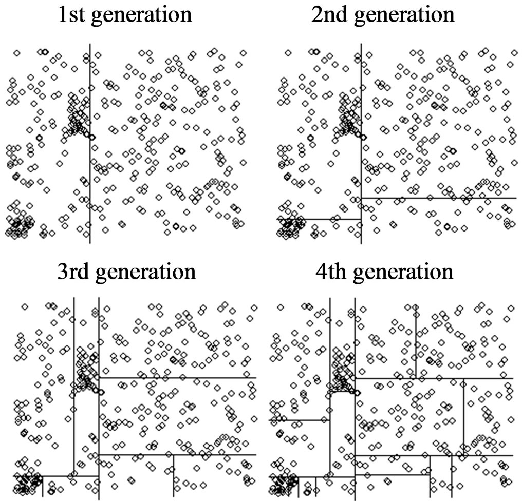
and possibly a 7th before stopping. Although the recursive partitioning in Figure 3 is demonstrated without a lattice structure and with no spatio-temporal smoothing, the process is very similar with these.
3.3. Pruning the Surveillance Tree to Deliver a Particular False Alarm Rate
The aim of pruning is to trim away all insignificant terminal nodes. If all nodes in the tree are pruned away then no outbreak is signalled, however if terminal nodes remain after pruning is completed, then an alarm is given. The geographical outbreak is diagnosed by the set of partitioning rules that define the terminal node. The pruning steps are now defined in more detail.
The process of pruning is very simple. We prune terminal nodes recursively starting with the last offspring in the tree. We prune the terminal node if
where these h-values are positive constants whose values are designed to deliver a specified false alarm rate. A sensible stopping rule for partitioning is to stop whenever
This avoids tree growing offspring that will not survive the pruning process. The pruning process leaves only generations with smoothed counts significantly higher than expected, e.g., if we started pruning from generation 4 in Figure 3 then only two offspring containing the outbreak regions plus their parents, grandparents, etc. would survive the pruning process. If pruning was applied to a tree for the left-hand plot in Figure 2 with no outbreaks, then each generation in turn would be pruned away until no offspring remain. Even the target region (the original parent) would be pruned indicating no significant outbreak.
4. Simulation Studies
The SCAN statistic with m = 21 is used. This scans just over  of the rectangular cells in the target area, i.e., the plan is designed for fairly large clustered outbreaks. The SCAN plan searches all possible 21 by 21 cells. This allowed
  unique regions to be scanned in the 100 by 100 cell region. If any one of these 21 by 21 regions has counts significantly higher than expected (i.e.,
 ) then the SCAN statistic signals. The simulation process was designed to examine homogeneous means with each cells assumed to have mean 0.01, and the EWMA surveillance tree is designed with
  and
and . All plans are designed to have an in-control ARL equal to 100.
The simulation process generated in-control counts and then adds to these additional counts for a fixed rectangular outbreak region. The location of the outbreak region is then hidden and we examined how early the plans alarm this outbreak. Rectangular outbreak regions were generated involving 21 by 11 cells, 11 by 11 cells, 50 by 20 cells, and 100 by 10 cells. So this provided outbreaks regions with areas ranging from 121 cells to 1000 cells, e.g., a range of sizes, shapes and positions. The detailed simulation results in terms of ARLs are reported in Appendix A (Tables A1 and A2). But the performance comparison between the two methods is outlined below.
The results show that the EWMA Surveillance Tree method does well when the outbreak is located on the boundary of the target region. This is where counts are smoothed less (e.g., where variances are higher). In the middle of the target region, the cell counts are smoothed the most, thus having the smallest variance for the smoothed counts. In addition, the performance of the EWMA Surveillance Tree method is quite satisfactory and it is more likely to flag large scale outbreaks earlier than SCAN plans with m = 21. This plan is also robust to changes in spatial non-homogeneity in means whereas other plans are not. This will be discussed in more detail later.
The ARLs in Appendix A result from 10,000 simulated run lengths for each plan. Although, the plans are compared within each Tables A1 and A2, we are more interested in the robust performance of plans, i.e., when nothing is known about the shape and size of the outbreak. If the outbreaks dimensions match the SCAN plan using 21 by 21 cell scans, then it is known to be close to optimal. On the other hand, the recursive partitioning plan’s properties are unknown and its flexibility appears to indicate its strength is in its robust performance across a range of outbreak dimensions, without being optimal for any specific outbreak size or shape. In other words, if the outbreak dimensions are known, then the SCAN plan can always be trained to be more efficient than the EWMA Surveillance Tree plan, and therefore is preferred in these circumstances.
In Table A1, the EWMA Surveillance Trees are better at finding the 11 by 21 outbreaks on the boundary, than the SCAN plan, but as the outbreak moves to the middle of the target region, the SCAN plans signals on average earlier. The message is the same for 11 by 11 outbreaks.
In Table A2, the EWMA Surveillance Tree method is better at finding the 50 by 20 and 100 by 10; with both recursive partition plans having earlier signals on average than the SCAN plan for all positive increases in mean. Tables A2 suggest if the outbreak is significantly wider spread than 21 by 21 cell region, then the EWMA Surveillance Tree approach has significant early signal advantages.
On average, the EWMA Surveillance Tree method compares quite favourably to the SCAN plan with m = 21 in terms of early signalling with much less computational effort, and therefore is a viable alternative. The real advantage is that these plans can easily be scaled up to higher dimensions while the SCAN plan cannot.
5. Recursive Partitioning Plans for Non-Homogeneous Spatio-Temporal Poisson Counts
We can also examine the EWMA Surveillance Trees for the m by m (where ) lattice structure for non-homogeneous spatio-temporal Poisson counts. An advantage of the method is that it is invariant to changes in mean within the range of 0.0025 to 0.2 per cell. That is, the same threshold is appropriate for a fixed lattice of m by m, independent of the changes in cell means of between 0.0025 to 0.2. However, the threshold is dependent on m, the dimension of the scanning window. A model for finding the threshold
  for given values of m is
This model delivers thresholds  that give ARLs within 5% of 100, provided
 .
.
6. Example of Application of Crashes in Sydney, Australia
This section of the paper applies the EWMA Surveillance Tree method to actual data from motor vehicle crashes in parts of Sydney, Australia from 2000 to 2004 (inclusive). Data are drawn from the Traffic Accident Database System (TADS) collated by the New South Wales Roads and Traffic Authority. Data are collected from police reports for all accidents where at least one of the following occurred:
• The accident resulted in either death or injury;
• At least one vehicle had to be towed away;
• At least one driver was reported as under the influence of alcohol;
• At least $500 worth of damage to property was attributed to the movement of a vehicle on the road.
These accidents are referred to as “crashes”. The data include the date, time and location of the crash. This application makes use of the date of the crash but ignores the time. The target region can be viewed in Figure 4. The suburb names are recorded at the location where the average accident occurs for that suburb.
The x and y-coordinates were divided into rectangular areas such that the marginal row (column) totals of the region included on average 2% of crashes. This gave a spatial region that was a 50 by 50 rectangular grid and a mean rate of 0.1 crashes per day per cell. The expected values for each cell could not be efficiently modelled because of the low counts and the number of cells too high. Therefore, a two stage approach was carried out— the total crashes per day across the whole target region were modelled using a Poisson regression approach similar to Sparks et al. [11] and this model was taken to establish the day-ahead forecast for total crashes. The history of crashes was then used to establish the proportion of total crashes expected to fall into each cell. The day-ahead forecast total counts multiplied by the respective proportions provide expected values for the daily counts of each cell in the grid. Data in 2000 where used to train the forecast models and outbreaks were explored for 2001 to 2004. The models were updated as in Sparks et al. [11] using a moving window of one year.
The EWMA Surveillance Tree plan was then applied to detect outbreaks in the number of crashes occurring across the region. Tables 1-3 summarises 3 periods with outbreak signals for 2001, 2003 and 2004, respectively. Most of the outbreaks flagged lasted for less than three days, but this paper highlights outbreaks that persisted for longer and thus provided opportunities for feedback control.
The outbreak in December 2001 (Table 1) spanned the full north-south and west of the target region. The geographical location of the daily signals was stable except towards the end when the crash region signalled starts to diminish in area before the signal disappears completely. The outbreak zone is fairly large and therefore is likely to be driven by persistent states that influence a broad range of drivers during that period, perhaps the busy Christmas season.
The outbreak outlined in Table 2 summarises an outbreak in July 2003. It begins by indicating nearly the entire target region as an outbreak, but then focuses on
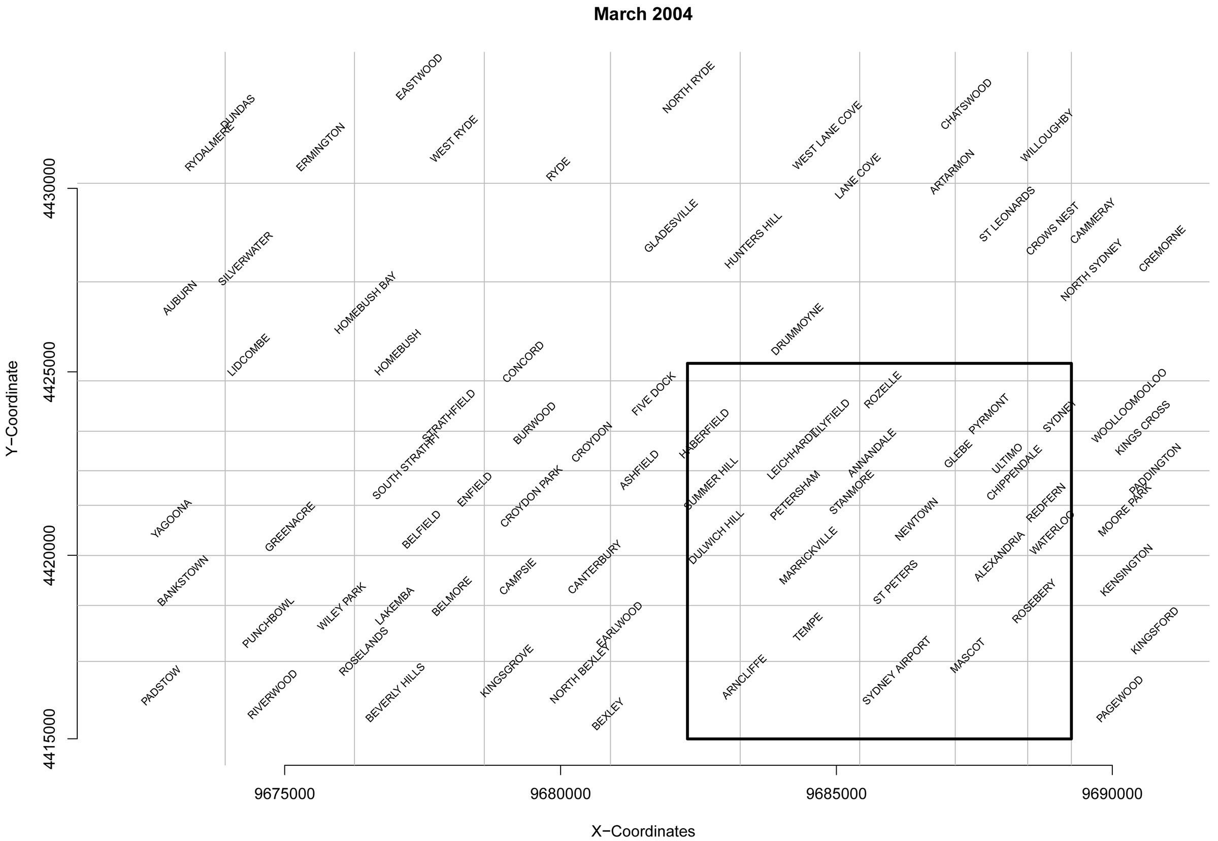
Figure 4. The centre of the outbreak region flagged in March 2004.
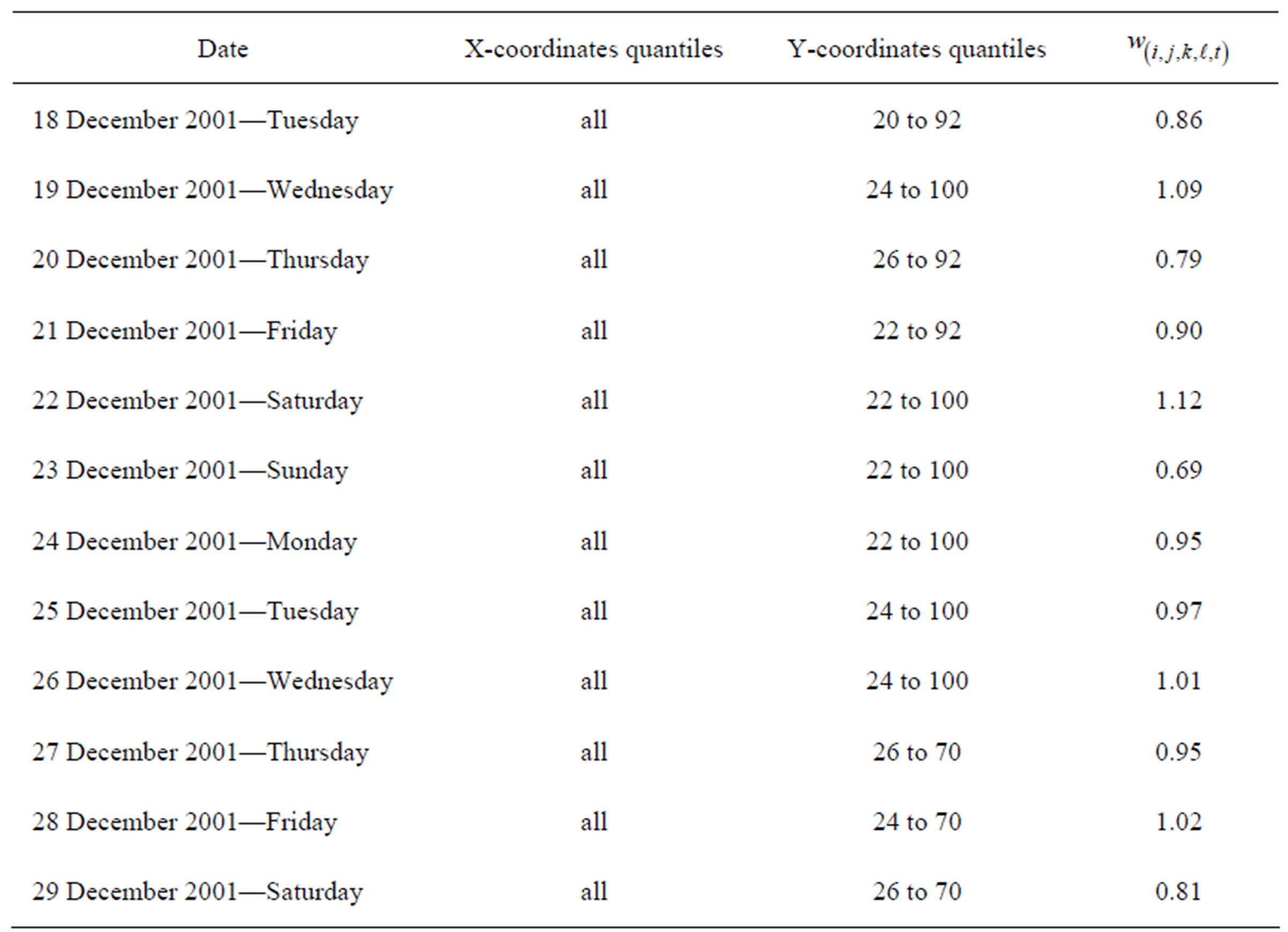
Table 1. Summary of a signalled outbreak in crashes for December 2001.

Table 2. Summary of a signalled outbreak in crashes for July 2003.
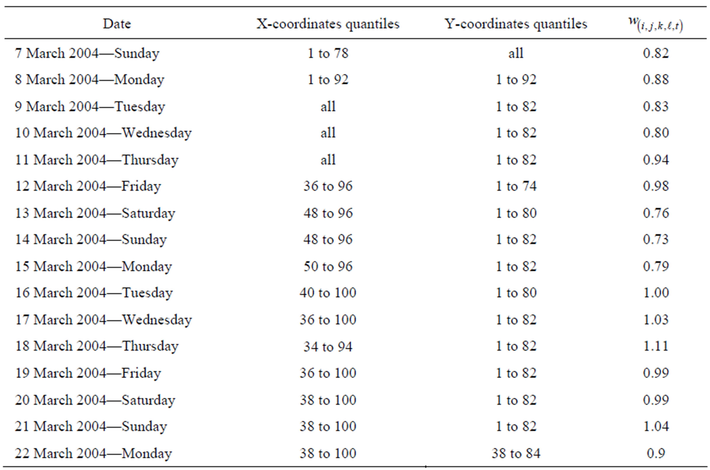
Table 3. Summary of a signalled outbreak in crashes for March 2004.
the centre and southern parts of the target region before moving back to nearly the entire target region. Again the outbreak zone is fairly large and therefore is likely to be driven by persistent states that influence a broad range of drivers during July 2003.
The outbreak outlined in Table 3 summarises an outbreak in March 2004. It begins by flagging a broad outbreak region that then changes more than the outbreaks given in Tables 1 and 2. Figure 4 indicates the region that is common to all of the outbreak signals (besides the last where the outbreak is diminishing to no signal). The outbreak region is centred around a region just south and south-east of the city, although it seems to shift.
7. Conclusions
EWMA Surveillance Trees offers a flexible and useful way of identifying unexpected geographical crash outbreaks. This is helpful in terms of managing driver risk by identifying the hot spots in the road network. This informs decision makers of the dynamic changes to driver risk which may then be managed through effective feedback controls (e.g., target policing). The fact that geographical risk persist at the same location over a few days means that harm from crashes could be reduced by such controls.
If the shape and size of future crash outbreaks are known, then the SCAN plan can be designed to detect these earlier than the recursive partitioning plan. However, in those cases where nothing is known about future crash outbreaks, the EWMA Surveillance Tree method offers an effective, robust and computationally efficient outbreak detection methodology. Another advantage is that it can be easily scaled up to include higher dimensions than two or three [12] whereas the SCAN plan becomes unworkable for any more than three dimensions. For example, other dimensions could include type of vehicle, nature of road movements during the crash, or the type of road/surface.
Lastly, due to its robustness at detecting clustered outbreaks, the EWMA Surveillance Tree methodology is applicable to a broader range of applications, such as, diseases, crime, and environmental applications.
REFERENCES
- M. Kulldorff, “Prospective Time Periodic Geographical Disease Surveillance Using a SCAN Statistic,” Journal of the Royal Statistical Society Series A—Statistics in Society, Vol. 164, No. 1, 2001, pp. 61-72. doi:10.1111/1467-985X.00186
- M. Kulldorff and N. Nagarwalla, “Spatial Disease Clusters: Detection and Inference,” Statistics in Medicine, Vol. 14, No. 8, 1995, pp. 799-810. doi:10.1002/sim.4780140809
- M. Kulldorff, “A Spatial SCAN Statistic,” Communications in Statistics: Theory and Methods, Vol. 26, 1997, pp. 1481-1496. doi:10.1080/03610929708831995
- M. Kulldorff, R. Heffernan, J. Hartman, R. M. Assunção and F. Mostashari, “A Space-Time Permutation SCAN Statistic for the Early Detection of Disease Outbreaks,” PLoS Medicine, Vol. 2, No. 3, 2005, pp. 216-224. doi:10.1371/journal.pmed.0020059
- W. H. Woodall, J. B. Marshall, M. D. Joner Jr., J. E. Fraker and A. G. Abdel-Salam, “On the Use and Evaluation of Prospective SCAN Methods for Health-Related Surveillance,” Journal of the Royal Statistical Society: Series A, Vol. 171, No. 1, 2008, pp. 223-237.
- S. W. Han, Y. Mei and K.-L. Tsui, “A Comparison between SCAN and CUSUM Methods for Detecting Increases in Poisson Rates,” Technical Report, School of ISyE, Georgia Institute of Technology, 2008.
- R. F. Raubertas, “An Analysis of Disease Surveillance Data That Uses the Geographic Locations of Reporting Units,” Statistics in Medicine, Vol. 18, 1989, pp. 2111- 2122.
- P. A. Rogerson and I. Yamada, “Monitoring Change in Spatial Patterns of Disease: Comparing Univariate and Multivariate Cumulative Sum Approaches,” Statistics in Medicine, Vol. 23, No. 14, 2004, pp. 2195-2214. doi:10.1002/sim.1806
- J. Glaz, J. Naus and S. Wallenstein, “SCAN Statistics,” Springer, New York, 2001.
- J. Chen and J. Glaz, “Two-Dimensional Discrete Scan Statistics,” Statistics and Probability Letters, Vol. 31, No. 1, 1996, pp. 59-68. doi:10.1016/0167-7152(95)00014-3
- R. Sparks, C. Carter, P. L. Graham, D. Muscatello, T. Churches, J. Kaldor, R. Turner, W. Zheng and L. Ryan, “Understanding Sources of Variation in Syndromic Surveillance for Early Warning of Natural or Intentional Disease Outbreaks,” IIE Transactions, Vol. 42, No. 9, 2010, pp. 613-631. doi:10.1080/07408170902942667
- R. S. Sparks and C. Okugami, “Surveillance Trees: Early Detection of Unusually High Number of Vehicle Crashes,” 2009. http://interstat.statjournals.net/YEAR/2010/abstracts/1001002.php
Appendix A: Simulation Study Results
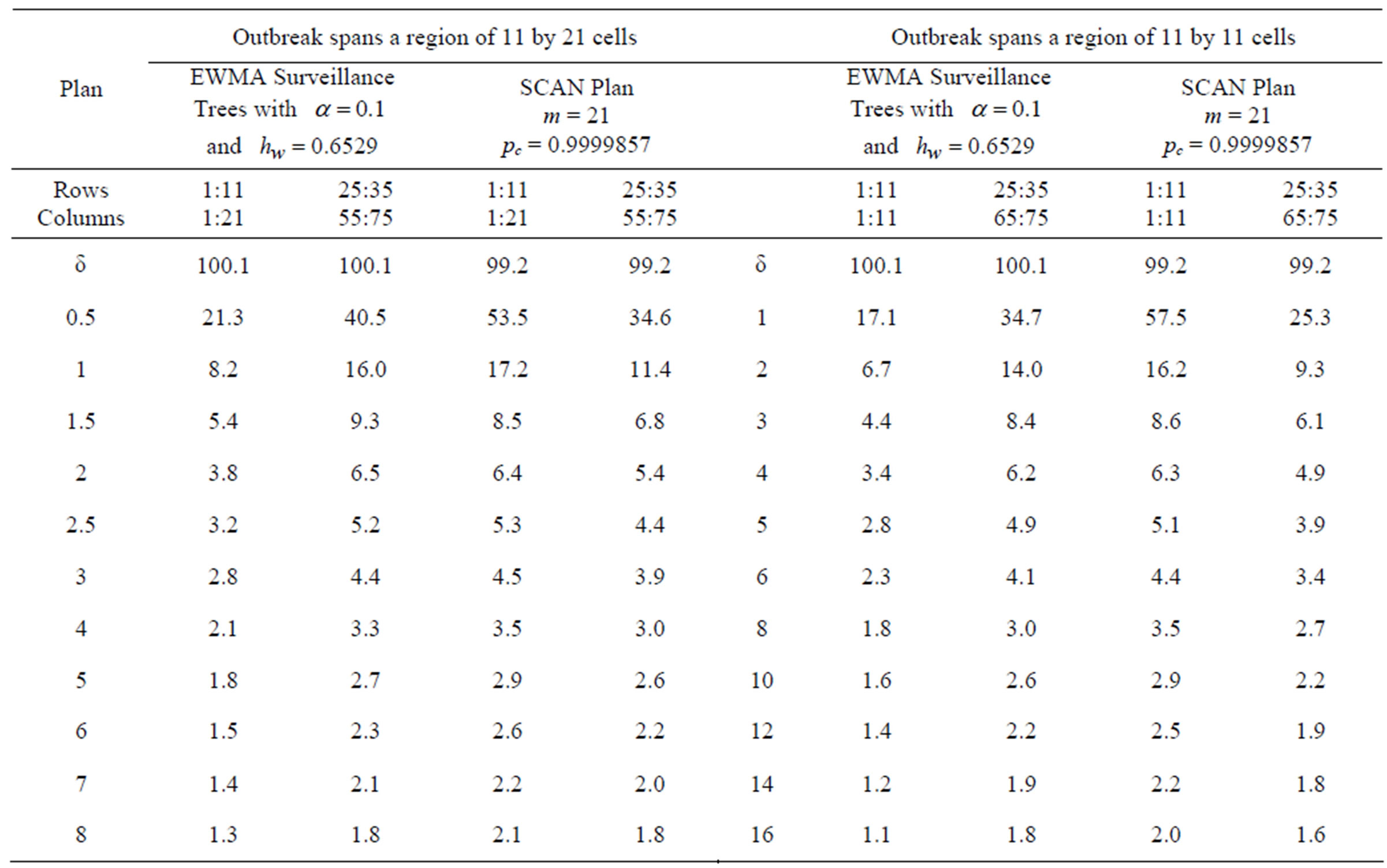
Table A1. ARL performance of the plans when the in-control ARL = 100 and the outbreak spans a region of 11 by 21 and 11 by 11 cells.
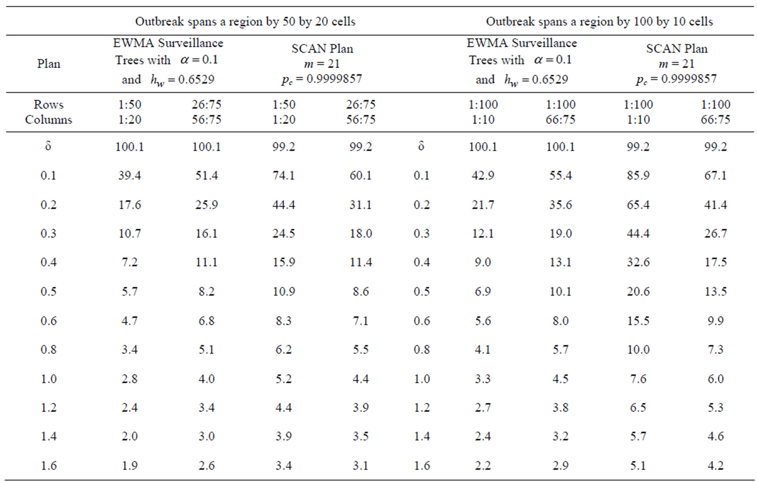
Table A2. ARL performance of the plans when the in-control ARL = 100 and the outbreak spans a region of 50 by 20 and 100 by 10 cells.