Open Journal of Marine Science
Vol.04 No.03(2014), Article ID:48423,20 pages
10.4236/ojms.2014.43019
Analytical Models for Hurricanes
Arkadii I. Leonov
Departments of Applied Mathematics and Polymer Engineering, The University of Akron, Akron, OH, USA
Email: leonov@uakron.edu
Copyright © 2014 by author and Scientific Research Publishing Inc.
This work is licensed under the Creative Commons Attribution International License (CC BY).
http://creativecommons.org/licenses/by/4.0/


Received 4 April 2014; revised 11 May 2014; accepted 30 June 2014
ABSTRACT
A two-layer theoretical model of hurricanes traveling (quasi-) steadily over open seas has been developed. The use of coherency concept allowed avoiding the common turbulent approximations, except a thin sub-layer near the air/sea interface. The model analytically describes 3D distribu- tions of dynamic and thermodynamic variables in hurricanes and analyzes processes of evapora- tion and condensation. Using this modeling, the following fundamental problems were naturally resolved-change in the cyclonic/anti-cyclonic directions of hurricane rotation and the directions of radial wind in lower and upper parts of hurricane; increase in wind angular momentum in hur- ricane boundary layer; dramatic effect of ocean spray and its radial distribution; and a high in- crease in temperature at the upper region of boundary layer. Additionally, integral balances al- lowed expressing the governing parameters of field variables via two external parameters, the sailing wind and temperature of a warm air band, in which direction the hurricane travels. A rude model for the hurricane genesis and maturing has also been developed.
Keywords:
Hurricane, Aerodynamics, Adiabatic and Boundary Layers, Air-Sea Interaction

1. Introduction
The hurricanes (typhoons) have been extensively investigated during the last 60 years. Many of their features have been observed and experimentally studied using satellites, aircrafts, ships, and buoys. These observations created a detailed qualitative picture of hurricane structure, documented in several well-known texts by Dunn [1] , Anthes [2] , Hsu [3] , Cotton & Anthes [4] , Ogawa [5] , and Emanuel [6] .
Some idealized models [7] -[12] of several problems in hurricanes have also been developed. Complicated role of mesovortices in the hurricane eye was experimentally modeled in laboratory and discussed [13] . Lighthill developed a thermodynamic theory of ocean spray [14] , and its effect on the dynamics of near water air turbu- lence was revealed by Barenblatt et al. [15] . Detailed models of coupled interactions between the turbulent wind and oceanic waves near the air/sea interface have also been elaborated in text [16] (Ch. 3). Other conceptual ideas are mixed with numerical studies. Some works [17] -[20] modeled intriguing aspects of hurricane maturing. Many other papers developed turbulent baroclinic and barotropic numerical models (e.g. see paper [21] and ref- erences there). To forecast hurricane travel these models interact with the current synoptic and lower scale ob- servations (see recent extensive reviews in Refs. [22] [23] ).
Yet several fundamental problems in hurricane physics remain unresolved. These are the change in the direc- tions of hurricane rotation and radial wind in lower and upper parts of hurricane, radial increase in wind angular momentum in hurricane boundary layer, dramatic effect of ocean spray and its radial distribution, and a high in- crease in temperature at the upper region of boundary layer. The problems of hurricane genesis and maturing are also currently vaguely addressed.
Thus the main objective of this paper is to resolve the above problems by developing and analyzing some quantitative models, based on the author’s results [24] -[27] pre-published in Arxive. The models being rude enough still provide a consistent analytical description of the basic physical phenomena in hurricanes. The con- ceptual view of hurricanes as coherent structures, allows avoiding the common turbulent approximations except friction factors at the air/sea interface. The use in the model the aerodynamics of ideal gas requires implement- ing continuity for dynamic variables to avoid the Kelvin-Helmholtz (K-H) instability. Additionally, integral balance equations allow expressing all parameters in the distributions of field variables via only two external parameters―the sailing wind and temperature of warm air band the hurricane travels along.
The paper is organized as follows. The next Section briefly discusses the external forces causing horizontal travel of hurricanes, thermodynamics of air, dynamics of ideal liquids, and hurricane structure. Section 3 models the basic airflows in the upper layer of hurricane. Section 4 models the basic processes in the hurricane boun- dary layer. The last, Section 5 presents simple analytical models for hurricane genesis and maturing.
2. Preliminaries
2.1. Horizontal Travel of Hurricanes
Two factors affect the horizontal travel of hurricane: 1) stirring or “sailing” wind with velocity
 and 2) “af- finity” motion with velocity
 because of hurricane’s tendency for accepting warmer air from environment. The value
 is unknown and should be found with solving problem. The additivity principle
 holds for describing horizontal hurricane travel.
2.2. Aerodynamic Equations for Air Flows
We consider air motions in hurricane as axially symmetric flows of ideal compressible gas. The frame of refer- ence used below is a cylindrical coordinate system with vertical
 -axis directed upward, slowly traveling in a horizontal direction. The axially symmetric motions of air relative to the local Earth rotation have very well known form (e.g. see Equations (1.7)-(1.10) in [24] ). In the stationary cases, these equations yield two first in- tegrals, which present the angular momentum M and temperature T as arbitrary functions of the stream function
 .
.
2.3. Thermodynamics of Humid Air
Far away from hurricane, the atmosphere is assumed to be horizontally homogeneous with vertically distributed ambient density
 pressure
 and temperature
 . These distributions are described by the equilibrium equations within the thermodynamics of humid ideal gas [28] .
Using adiabatic description of air,
 , (1)
, (1)
and the static equation,
 , (2)
, (2)
the vertical distributions of thermodynamic parameters are presented as:
 . (3)
. (3)
Here
 with
with
 being ambient parameters at the surface,
 is the adiabatic index, and
 and
and
 are the heat capacities at constant pressure and constant volume, respectively.
2.4. Hurricane Structure and Basic Processes
A typical structure of a mature hurricane traveling (quasi-) steadily over the open sea is sketched in Figure 1. The hurricane is viewed as a solitary vertical air vortex rotating in the cyclonic direction near the bottom with additional radial and vertical air flows. It has a central “eye”, a vertical column of radius , sur- rounded by the “eye wall” (EW) layer with external radius
 of ~30 - 50 km. Above the hurricane boundary layer (HBL) with vertical thickness
 , the radius
 of external EW changes with height
 . Along with a radial air flow, the air within the EW performs intense rotation, whose peak is achieved at
 . An upward weak vertical speed component of airflow is mostly contained within the EW region. We call this rotating and as- cending airflow as EW jet. In the external region, outside the EW, the relative rotation of hurricane decreases to zero at the external hurricane radius
 . The radial airflow is inwards at the bottom and out- wards at the top of hurricane. The entire vortex could be vertically layered into the bottom HBL, and upper “adiabatic” layer, with the total hurricane height up to 20 - 30 km.
The vertical structure employed in the following models, includes the turbulent boundary sub-layer of thick- ness , HBL of height
 , and very high “adiabatic” layer ascended up to tro- posphere. The affinity motion (if exists) is driven by environmental near-sea warm air band with the temperature
 , which supplies a warmer air to the hurricane boundary layer. The geometry of the warm air band is simplis- tically viewed as a parallelepiped of height
 and width H. When
 , hurricane optimally adjusts the bottom EW size to the warm air band size.
In the HBL, the air-sea interaction directly affects the dynamics at the air/sea interface, generating oceanic waves which in turn interact with air flows in the outer part of HBL. There is also evaporation and the heat/mass exchange between the hurricane and environment. The moisture, sensible and latent heats are transported via HBL towards the EW jet. The height of HBL is limited by air moisture condensation, which causes the forma- tion of spiral rain bands, layered clouds and rainfall from them. Dynamic effects of rainfall can seemingly be neglected, though the rainfall can balance the evaporation from the oceanic surface. This results in a constant sa- linity level in the oceanic boundary layer.
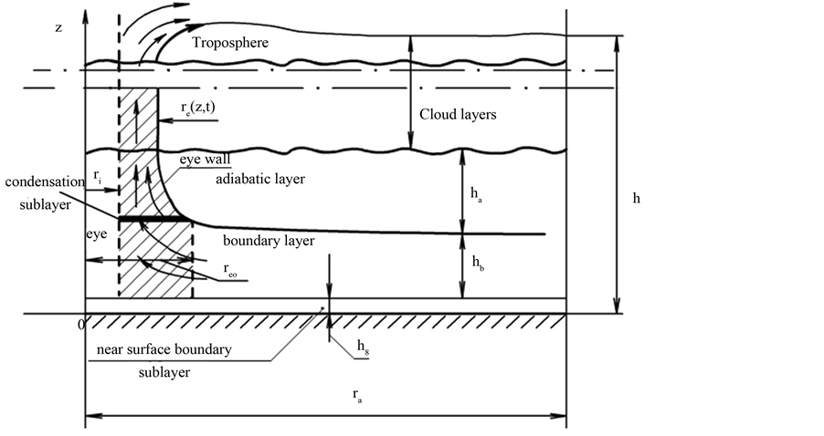
Figure 1. Schematic structure of a hurricane.
3. Model of Adiabatic Layer for Steady Hurricane [25]
Neglecting the air band effects, air flows in upper layer of hurricanes can be modeled using the adiabatic ap- proximation. The structure and basic flows in the hurricane adiabatic layer is sketched in Figure 2, and the air- flows there are axi-symmetric. Here is a solid-like rotation of air in the eye region, and no vertical wind compo- nent exists in the outer region of hurricane. For convenience, we use in this Section the vertical axis z shifted upward by the height
 of boundary layer.
The following modeling equations are used below [25] :
 (4)
(4)
 (5)
(5)
In aeromechanical Equations (4),
 is the angular air velocity relative to the angular velocity
 of Earth rotation on
 -plane. Equations (5) represent the “jet approach” [29] for vertical mass balance and momentum in the eye wall averaged over radius. Introducing the stream function by common relations,
 ,
,
 , yields the first integrals. Their linear forms
 ,
,
 with numerical coefficients
 and
and
 allow an easy physical interpretation.
We now introduce two simplifying approximations:
(i) ; (ii)
 (6)
(6)
Here (6i) presents the “well mixing” assumption introduced by Deppermann [30] , and independency from air rotation introduced in (6ii) has been justified in Ref. [25] .
It is convenient to introduce the non-dimensional variables:
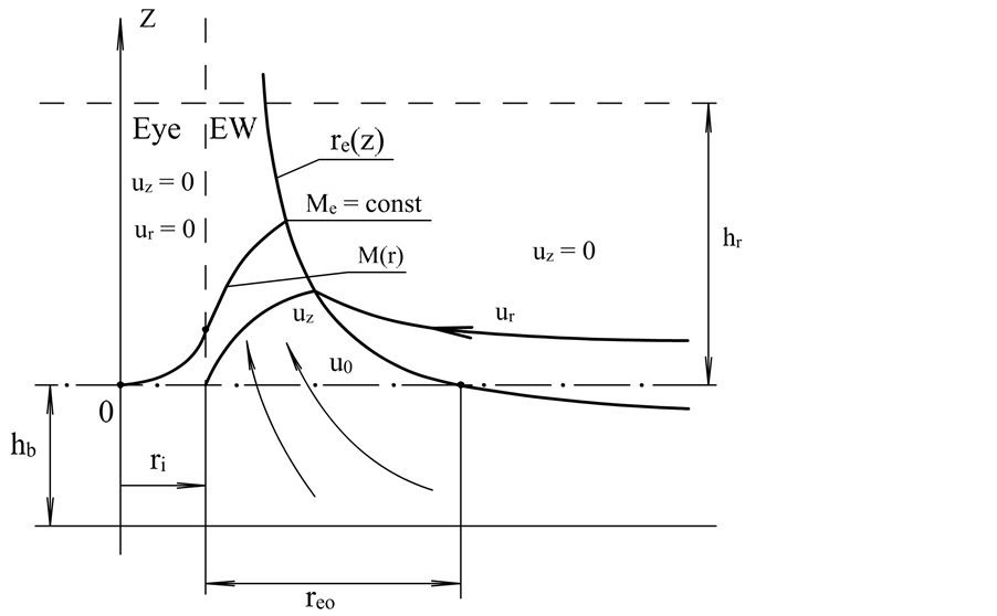
Figure 2. Sketch of adiabatic layer.
 (7)
(7)
Here
 is the kinematic condition which relates the vertical and radial velocity at the outer jet radius. The common boundary conditions of continuity are employed for radial and rotational components of air field, with “frictional” kinks in distribution of angular momentum at the inner and outer walls of EW. Other na- tural conditions used in calculations are:
 when
when .
.
Tedious calculations of set (4) with approximations (6) yield the explicit expressions for radial non-dimen- sional distributions of dynamic variables:
 ,
,
 (8)
(8)
 ;
; ;
;
The approximation
 or
or
 was used in formulas (8). Here
 is the external radius of hurricane. In (8), parameter
 characterizes the effect of rotation on the EW jet cross-section, and parameter
 describes the frictional kink in the distribution of angular momentum at
 [25] . The struc- tural functions
 and
and
 are given by (A1) in Appendix.
Formulas (8) show that streamlines in hurricane are the circles in eye and outside EW, and ascending spirals in EW with kinks at ,
, . Equations for jet radius and vertical velocity profile are then found upon substituting (8) into (5). It yields the equations for mass conservation, and evolution of the jet profile. These eq- uations are written in the non-dimensional form (7) as:
 ; (9)
; (9)
Here ,
,
 is the buoyancy parameter, and
 . The values
 and
and
 in (9) correspond to
 , the structural function
 is given by (A2) in Appendix, and
 .
.
There are simple asymptotic solutions of (9) in two limiting cases.
1) :
:
 (10)
(10)
Here
 are some algebraic functions of
 and
and
 presented via formula (A2) [25] . The only physi- cally feasible case is
 where for stability, the heat supply from HBL to the hurricane jet should exceed the adiabatic cooling. Here the initial jet profile is convex down, with centripetal radial flow
 .
.
2) :
: ;
;
 (11)
(11)
When , the vertical component of air flows vanishes being converted to the radial one, with the jet ra- dius approaching to infinity.
It was found that the numerical solution of steady problem (9) exists only for physically feasible case . The following realistic parameters were accepted below in the demonstrative calculations:
 ,
,
 ,
,
 ,
, ;
; ,
,
 or 0.00363 (~3 or 1 m/s),


 .
.
The values of calculated parameters are: ,
,
 ,
,

 ,
,
 ,
,
 ,
,
 , and
, and .
.
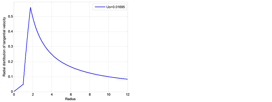
Figures 3-9 illustrate the calculated radial distributions of basic variables, depending on altitude and initial value of vertical velocity . Figure 3 demonstrates the characteristic non-monotonic behavior of outer EW jet boundary, Figure 4 the increase in vertical velocity. Figure 5 shows that the angular velocity in EW jet de- creases with altitude, though the region when it is negative is not shown. Radial distributions of angular mo- mentum M and tangential velocity
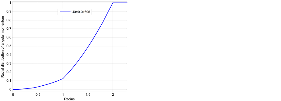
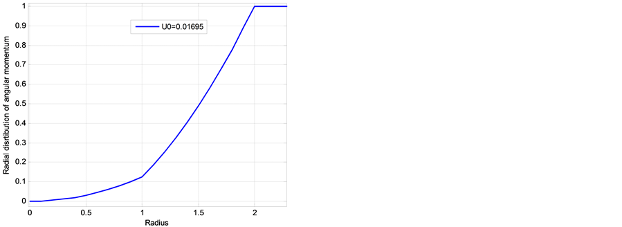
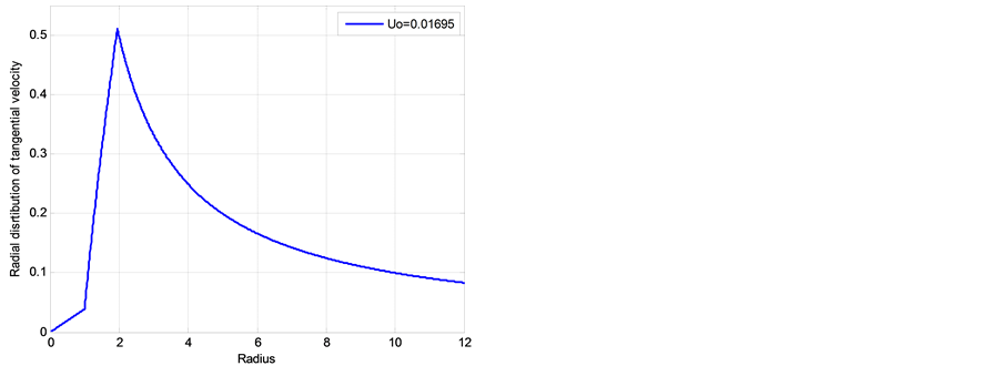
 for two altitudes, presented in Figure 6 and Figure 7, demonstrate their increase in the eye and EW regions with two characteristic kinks, a plateau for M outside EW jet, and a sharp peak of
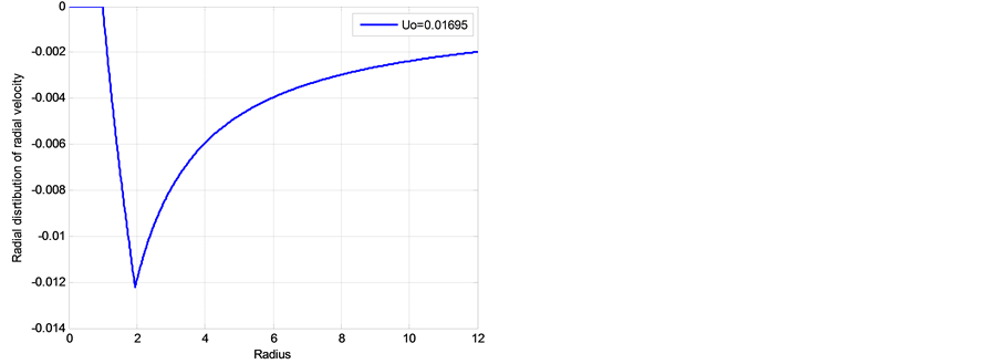
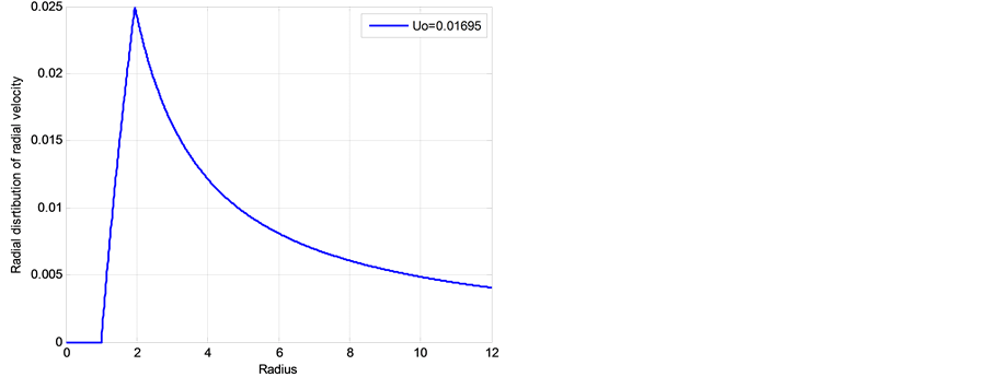
 at the outer boundary of EW. Figure 8 show characteristic distributions of radial velocity. It is
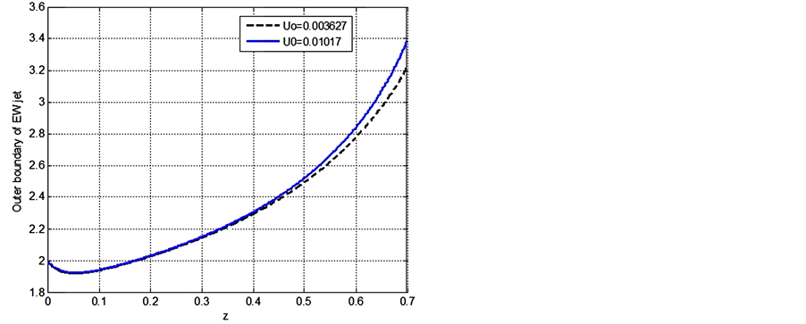
Figure 3. Non-dimensional altitude dependence of outer boundary of EW jet ;
;
 (solid line) and 0.003627 (dashed line).
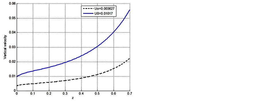
Figure 4. Non-dimensional altitude dependence of vertical velocity
 in the EW jet. Parameters are the same as in Figure 3.
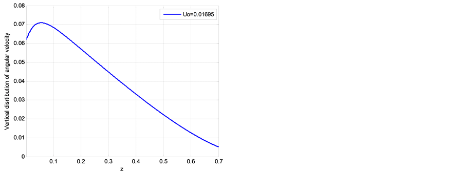
Figure 5. Vertical distribution of non-dimensional angu- lar velocity
 of EW jet.
 (a) (b)
Figure 6. Non-dimensional radial distributions of angular momentum
 at two non-dimensional altitudes: (a)
 ; (b)
; (b) .
.
 (a) (b)
Figure 7. Non-dimensional radial distributions of tangential velocity
 at two non-dimensional altitudes: (a)
 ; (b)
; (b) .
.
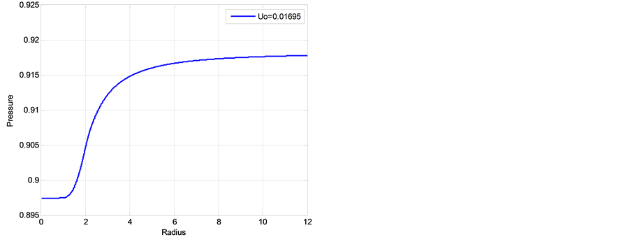
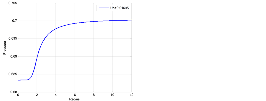
negative (centripetal) at lower and positive at higher altitudes, with absolute maximum at the outer boun dary of EW jet. Finally, Figure 9 show two similar radial distributions of pressure which display a characteristic “depression” area at the center of hurricane. These results support a well-documented characteristic structure of hurricane sketched in Figure 10. Additionally, the radial distributions of tangential velocity and pressure at the bottom of adiabatic layer were found in [25] in a good agreement with these obtained using semi-empirical modeling and observation data by Deppermann [30] .
4. Modeling the Boundary Layer in Steady Hurricane [26]
The structure and basic interactions in hurricane boundary layer (HBL) are sketched in Figure 11. Here the HBL is horizontally separated in the same three regions as in previous Section: the eye, HBL EW, and outer HBL region, the latter having generally a curvilinear upper surface. There are two major vertical sub-sections in HBL: upper aerodynamic and lover turbulent ones. Additionally, there is a condensation sub-layer located at the top of HBL EW and assumed to be very thin (~100 m). The height
 of HBL is restricted to the condensation level
 whose value is roughly evaluated using an empirical condition for the beginning condensation when the saturation point is achieved
 [4] . Here
 is the dew point temperature
 (a) (b)
Figure 8. Non-dimensional radial distributions of radial velocity
 at two non-dimensional altitudes: (a)
 ; (b)
; (b) .
.
 (a) (b)
Figure 9. Non-dimensional radial distributions of pressure
 at two non-dimensional altitudes: (a)
 ; (b)
; (b) .
.
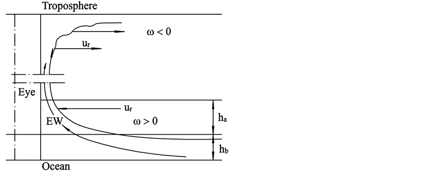
Figure 10. Sketch of the total vertical distribution of EW jet.
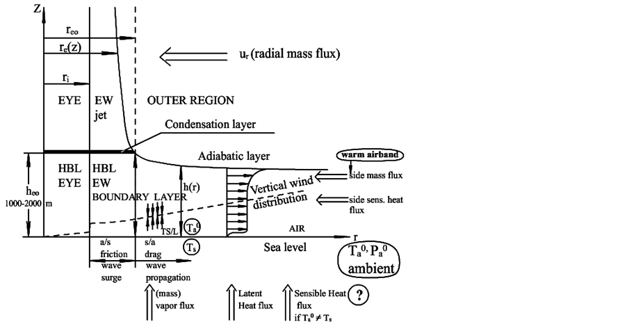
Figure 11. Cross-sectional sketch of HBL and diagram of air/sea interactions.
depression at the sea surface. The common evaluation
 yields
 .
.
4.1. Fluid Mechanical Effects in HBL
They include coherent aerodynamic airflows in upper part of HBL, turbulent airflows in lower part of HBL, and dynamic interaction of oceanic waves with HBL airflows.
4.1.1. Aerodynamic Airflow
Models employ simplified equations of aerodynamics of ideal gas similar to Equations (4) with , but omitting the
 effects:
 (12)
(12)
Omitting the
 effects in (12) makes these equations inapplicable far away from the HBL EW. The last formula in (12) presents a typical boundary layer approximation. Here
 is the barometrically corrected radial pressure distribution at the bottom of adiabatic layer described at
 by Equation (8).
The same assumptions as in the previous Section are employed here: the rigid-like airflow in HBL eye, the radial independence of vertical wind in HBL EW, and the same boundary conditions at the inner HBL EW in- terface. It is also assumed that the outer upper boundary
 of HBL is inpenetrable for the vertical wind component. Although far away from HBL EW the airflow is not axisymmetric, it is still modeled as pseudo- symmetric one.
Introducing the stream function
 as
as
 and
and , yields two first integrals written in the linear form as:
 ,
, . It is convenient to introduce here new non-dimensional coordinates, vertical
 , and radial
 ones. Here
 , and
, and . It is initially assumed that the angular momentum
 at
at , which will be justified later. Then the explicit solu- tion [26] of set (12) is presented by for EW and outer region of HBL as:
 (13a)
(13a)
 (13b)
(13b)
Here
 is the same frictional kink parameter and total radial air flow flux is:
 . Here
 is the induced radial velocity at the lower boundary of adiabatic layer at
 , and
, and
 is a “pseudo-radial” contribution of hurricane travel speed
 . The non-dimensional function
 characterizing the vertical structure of velocity field cannot be determined using the ideal aerodynamics. It is assumed to be positive, slightly varied and monotonically increased
 . Formulas 13(a), 13(b) show that except vertical wind component
 , two other wind components and angular momentum
 are continuous at the radial boundaries
 and
and .
.
At the upper boundary HBL EW,
 satisfies the natural boundary condition
 , which guaranties continuity for dynamic variables here. Also, since the upper boundary
 of HBL is assumed to be im- penetrable, the condition
 defines a particular streamline separating the HBL from the adiabatic layer. The evident kinematical relation
 holds at
 . Since
 and
and
 in HBL the model predicts decreasing thickness of HBL towards periphery
 . Rewriting the boundary
condition at
 in the form
 , shows that the sharper increase in
 the slower is
 decrease. The above results demonstrate that the streamlines in the HBL look like ascending spirals with ultimate streamline being the upper boundary
 of HBL. Since at
 both
both
 and
and
 are con- tinuous, the radial velocity component is also continuous at this boundary, although the vertical velocity com- ponent has a small jump there, similar to that found in the previous Section. It is also proven that the external boundary of EW jet smoothly continues downward, to the HBL upper boundary below the level
 . Finally, at
 , we impose a rude condition
 , although at the lower level of HBL the aerodynamic model is invalid.
4.1.2. Airflow in Turbulent Sub-Layer
A huge air wind near the radius
 maintains a surge of broken oceanic waves under EW bottom with
waves propagating outside this region. The radial wind contribution can be neglected in this sub-layer because of very low variation assumed for . Since no model currently exists for describing the interaction of air- flow with broken oceanic waves, a semi-empirical approach is used below. It is based on the fact that at the anemometer height
 the horizontal wind speed is equal almost 75% of the air speed at the level of aircraft observation (see e.g. paper [31] and references there). This fact may happen because of direct dynamic effect of ocean spray [14] [15] .
We use for friction factor
 the common bulk relation
 where
where
 is the mean velocity at the
height , yet to be established, and
 is the friction (drag) coefficient. The standard logarithmic pro- file is used for describing the mean velocity. It parameterized with roughness factor
 and reciprocal Karman constant
 . Matching the logarithmic profile with the aerodynamic profile (13) and using flatness of
 yields [26] :
 (14)
(14)
Evaluation of the roughness factor
 and the height of turbulent sub-layer
 at
at
 (or
(or ) are presented in Table 1. Finally, extending the observation in paper [31] to the entire turbulent sub-layer of HBL and using (14), yields the distribution of tangential velocity at the anemometric height
 :
:
 (15)
(15)
4.1.3. Interaction of Air Wind and Oceanic Waves
The radial increase in angular momentum
 as
as
 observed in the region
 , was explained by Emanuel [7] who used some thermodynamic arguments, assuming that the height of HBL is constant. This as- sumption necessitates a vertical airflow through the upper HBL boundary. Another idea proposed by Dr. A. Be- nilov and elaborated by the author is presented below.
Consider the oceanic waves initiated in the vicinity . They propagate into the outer area
 along the straight lines tangential to the circle
 with the constant phase speed
 (Figure 12). Therefore there is a skew interaction of the oceanic waves with air, resulted in dominant tangential airflow in the turbulent layer. Then the tangential shear stress
 along the wave path changes from the initial value
 to the val- ue
 at the current radius
 , as
, as ,
,
 . Using these formulas yields:
 ;
; ,
,
 ,
,
 ,
, . (16)
Here the low indexes “e” and “r” denote the values of variables at the radii
 and
and , respectively, and
 is the local phase velocity of wave. Due to (16),
 is directed at the circle of radius
 under angle
 defined as:
 . Hereafter the upper index “T” denotes the values of variables in the turbulent sub-layer of HBL region 2. Formulas (16) explain the observed behavior of the tangential wind, and slightly differ from the second expression in (15). The result shows that in the turbulent sub-layer of outer HBL region, oceanic waves rather generate air wind than dissipate it. Since the ratio of air to water density is
 the energy loss in wave to air transfer is negligible. Using then the wave energy conservation, results in the wave energy decay as ~1/r.

Table 1. Values of roughness parameter
 and height of turbulent boundary layer
 .
.
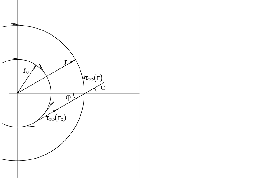
Figure 12. A sketch of skew interactions of oceanic waves with turbulent air in HBL.
4.2. Physical Effects in HBL
Evaporation from the oceanic surface and latent heat. Over calm oceanic water, the vertical air flux (per unit mass of vapor) caused by moisture evaporation can be approximated as
 [2] . Here
 is the wind speed at the anemometer level
 (~10 m), and the exchange coefficient
 . The ocean spray ejected over the oceanic water by the wave whitecaps, can increase the value of
 at least by an order of magnitude at the hurricane EW [14] . The studies [32] [33] found that whitecap concentration is
 , where
 . We adopt here
 as found in recent satellite observations. These results are incorporated in the model, under assumption that transfer coefficient
 is radial dependent decaying from its maximum value
 at
at
 as a cube of relative velocity:
 , and
, and
 (17)
(17)
Here
 is the near water wind speed given by (15), and for developed hurricanes
 is the maximum value of
 at
at .
.
Consider an example. Using (15) with
 and
and , we find from (17) that at

 the value
 is ~15 times lower than
 . It is in the range
 re- ported in Anthes book [2] . If the value of maximal tangential wind is
 , Formula (17) shows that
 , i.e. the process of effective evaporation continues in the entire hurricane area
 .
.
Using (15) and (17), the total mass flux of evaporation
 and the latent heat
 are calculated as:

 ;
; . (18)
Here
 is the vapor density,
 is the maximal tangential wind speed, and
 is the non-dimensional value of the wind speed shown in (15). Also, in (18)
 is the specific latent heat of vaporization,
 is humidity, and
 is the value of latent heat excess over the environmental air at the sea surface.
Transfer of sensible heat is considered in the steady model under condition of complete sea/air temperature balance . Therefore direct heat exchange between ocean and HBL does not exist. It is in accord with the Chapter 3.9 of text [6] and in contradicts the assumption of the models [6] [23] . A small dissipative heat neglig- ibly increases
 [26] . It means that in steady hurricanes the sensible heat could be transferred only from the horizontal warm air band.
Condensation is assumed to happen in a relatively thin vertical layer whose height is less than hundred meters, where the over-saturated vapor comes into the upper layer of HBL. Neglecting the thickness of the layer, it is considered as a weak condensation jump, which is described by basic equations including the conservation of vertical fluxes of mass, momentum and energy [34] . For a weak jump these equations are reduced to the conti- nuity of mass flux, pressure and enthalpy on the jump interface, averaged over EW radius:
 (19)
(19)
Since the differences between velocities, pressures and densities over the jump are negligible,
 ,
,
 ,
, . Those simplifications are the same as in slow combustion theory [34] .
4.3. Integral Balances in the HBL Eyewall
The average temperature
 and vertical velocity
 at the bottom of adiabatic layer are still unknown. Also generally unknown are the velocity
 of the horizontal motion of hurricane and the value of angular momen- tum
 in adiabatic layer. Using integral balances and given the geometrical structure of hurricane, these un- known parameters are expressed below through the known external parameters of hurricane, the sailing wind velocity
 and known temperature
 of warm air band. This also allows disregarding the vertical structure of dynamic variables in HBL, described by the function
 .
.
In the following we use the plane Cartesian axes ,
, ; the axis
 coinciding with the axis of the warm air band. Then the parallel
 and normal
 projections of the sailing and affinity components of horizon- tal wind are:
 ,
, . (20)
4.3.1. Mass Balance of Dry Air in HBL
Two fluxes of the “dry” air masses come from HBL to the EW jet via the bottom of adiabatic layer: 1) the flux from the radial airflow into the HBL and 2) fresh air coming because of horizontal travel of hurricane. Neglect- ing density variations, the balance is:
 ,
, (21)
(21)
Here
 is the width of warm air band,
 , where
 (see Equa- tion(10) and references there). The left-hand side of (21) describes the air flux leaving the HBL; the first term in the right-hand side the rate of mass supplied by induced radial flow at the bottom of adiabatic layer, and the second is caused by horizontal hurricane motion.
4.3.2. Balance of the Sensible Heat in HBL Reads
 (22)
(22)
In (22) the differences between heat capacities are neglected. The left-hand side of (22) describes the heat en- tering the hurricane condensation layer with unknown temperature , and the right-hand side the air heat sup- plied by the warm air band.
4.3.3. Oceanic Vapor Mass Balance Is
 . (23)
Here
 is the mass flux of oceanic vapor presented by (18), and the right-hand side is over-saturated vapor flux into adiabatic layer from the condensation surface at
 .
.
Balance of the latent heat is presented by second formula in (18).
Assuming that the oceanic vapor is completely condensed in the condensation layer, the last formula in (19) along with (23) yields two useful chain equalities:
 ;
; . (24)
The values of , depending on parameters
 and
and , easily found numerically. E.g.
 when
when
 and
and .
.
Entropy balance, detailed in [26] , starts with the well-known equation:

Here entropy
 is normalized on ambient conditions and the dissipa- tion is localized at the sea-air interface in HBL EW. Integrating the above equation over the volume of HBL, except a thin bottom layer of EW of thickness
 , and noticed that the latent and sensible heat had been ba- lanced, the
 balance is reduced to the integral pressure balance. Tedious calculations yielded:
 (25)
(25)
Here numerical parameter
 depends only on value of
 , e.g.
 for
for .
.
Affinity velocity of hurricane travel was determined in [26] , assuming the stream from warm air band is effec- tively mixed by dominant tangential air wind,
 (26)
(26)
Thus, all the unknown parameters,
 and
and
 can be effectively found from the above equations with given values
 ,
,
 , hurricane geometry, and parameters
 and
and . Although the following calcula- tions are explained in details in [26] , these explanations are also briefly shown below because of some arith- metic mistakes and misspellings in the above report and new account of evaporation in this paper.
Recall that the non-dimensional temperatures ,
,
 and
and
 are defined as:
 ,
, ,
, .
.
It is convenient to introduce non-dimensional wind components, scaled with the adiabatic speed
 as
as . Then (24) takes the form:
 (27)
(27)
The above relations yield the five equations for parameters
 and
and :
:
 (28)
(28)
Here ,
,
 , the functions
 ,
,
 are tabulated in report
[25] , and non-dimensional constants ,
,
 ,
,
 , and
, and
 are presented as:
 , (29)
Substituting
 in the first equation in (28) yields an awkward algebraic relation between tangential wind speed, and given values of horizontal temperature and sailing wind component. For illustrating purpose, only two limiting cases of this equation are considered below.
1) External sensible heat supply is negligible― . The hurricane is only driven by sailing wind
 . Then
 , and the dimensional solution is:
 (30)
(30)
One can see that due to (30)
 and
and
 are monotonically increasing functions of
 , whereas
 might decrease with
 growing.
2) Sailing wind is negligible― . In this case the hurricane moves with affinity speed
 , and the solu- tion, presented in dimensional form is:
 (31)
(31)
Formulas (31) show that ,
,
 ,
,
 , and
, and
 increase with
 growing, while
 might depend on
 non-monotonously.
In the limit cases,
 in (30) and

 in (31) the solution is:
 . (32)
Formulas (32) show that the steady, rotating hurricane can exist even without horizontal travel. Here the heat supply
 to the adiabatic EW jet is entirely produced by the condensation heat only due to moisture vaporiza- tion.
4.4. Numerical Illustrations
1) Accepted and calculated parameters
Geometrical parameters known for the “standard” hurricane are:

 , and
, and . Calculated geometrical parameters are:
 ,
,
 ,
,
 ,
,
 ,
,
 ,
,
 , and
, and .
.
Physical parameters are― with
with ;
;
 and
and
 [28] ;
 ,
,
 ,
,
 , and
, and .
.
Note that values
 and
and
 being chosen here arbitrarily are still reasonable. Evidently, decreasing
 and increasing
 will increase the severity of hurricane.
Parameters calculated from (29) are shown in Table 2.
2) Results of calculations. Using Table 2, the basic variables of hurricane for both cases were calculated and shown in Table 3 and Table 4. It was shown in [26] that the stability condition
 is satisfied here.
In both the cases, the most striking result of calculations is a high increase in temperature
 at the upper part of HBL EW, close to the observed values [2] . It clearly indicates the leading role of condensation. High in- crease in temperature
 of warm air band only slightly contributed in
 . Also, the vertical wind speed component
 is only slowly growing in both cases, tangential one
 is also growing, albeit not highly, but more in the affinity case. The radial wind speed component
 slightly decreases with growing either
 or
or . It means that due to the mass balance, the increasing rate of air entering the adiabatic EW jet from the HBL creates the lower value of initial tangent
 of the hurricane EW jet.
Table 2. Calculated non-dimensional parameters of standard hurricane.
Table 3. Results of calculations of basic variables in hurricane travel under given values of sailing wind

 . The values of temperatures are in
 ; velocities in m/s.
Table 4. Results of calculations of basic variables in affine travel of hurricane under given values of

 .The values of temperatures are in
 ; velocities in m/s.
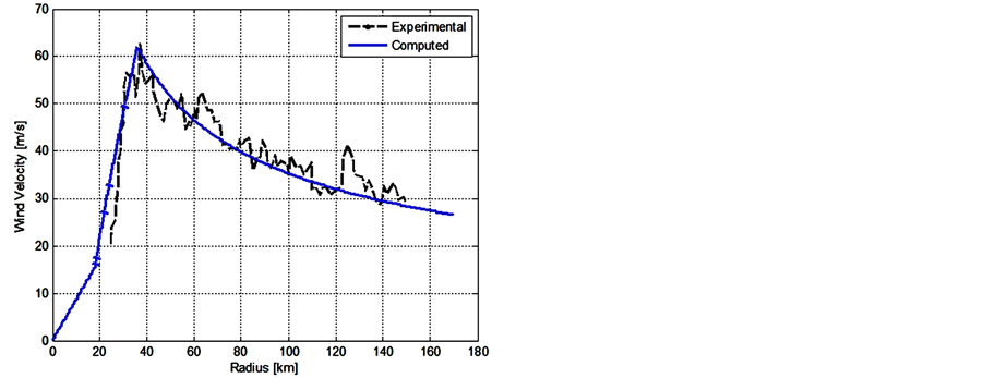
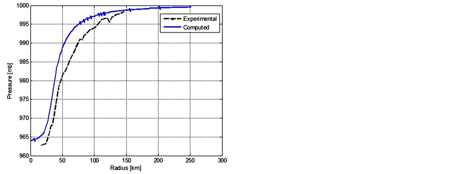
Calculations of the radial distributions of surface pressure and wind for hurricane Frederic, 1979, using the data according to paper [31] , were detailed in Ref. [26] . Comparison of data with our rough calculations is shown in Figure 13(a) and Figure 13(b).
5. On the Hurricane Genesis and Maturing [27]
The emergence of hurricanes is still mysterious. Many observations of initial stages of hurricanes (e.g. see the text [2] ) found a threshold value of vorticity, exceeding which the hurricane is maturing. Analyses in papers by Ooyama [17] [18] and Emanuel [19] [20] have a mutual defect-adjustable diffusivity of angular momentum to fit the data. Also, most hurricanes in Atlantics are formed in near equator zone, indicating the importance of Co- riolis factor, which was not considered in the above papers.
Paper [27] proposed a two-steps scenario of hurricane’s genesis. In the first step, an emerged plume of warm and humid air formed in the near equator zone, moves upward (see the model of plume dynamics in [27] ). In the second step, the plume captures the rotation from a horizontally sheared wind, with restructuring of the plume and acquiring an initial value of angular momentum. If this plume is stable, the maturing stage begins. In this case the hurricane grows in the radial direction, presumably caused by the K-H instability with radial propaga- tion into ambient air under action of Earth rotation.
To describe the maturing stage of hurricanes we first consider the quasi-static relation for angular momentum extended to the external boundary
 of hurricane:
 . (33)
The absolute
 and relative
 tangential velocities are then defined as:
 (34)
(34)
The slow evolution of
 and
and
 is now described by two heuristic equations:
 (35)
(35)
The first equation in (35) describes propagation of the hurricane front due to the K-H instability with the rela- tive rotational velocity at the boundary . The second equation in (35) assumes that the radius change due
 (a) (b)
Figure 13. Comparison of our adiabatic calculations and measurements [31] for radial distributions of tangential wind and surface pressure for hurricane Frederic for measurements on 09/11/1979: (a) Tangential wind; (b) Surface pressure; maximal wind speed , radius of eye jet
 Dashed and solid lines are measurements and calculations, re- spectively.
to the radial propagation of unstable boundary is the dominant contribution in the change of angular momentum.
The initial conditions are:

 ,
, . (36)
Here
 is the horizontal shear of wind initiated the plume rotation.
The solution of Equations (33)-(35) with conditions (36) is:
 (37)
(37)
Formulas (37) show that depending on sign , the plume can rotate in cyclonic or anti-cyclonic directions.
1) In the cyclonic case , hurricane propagates outwards. It is the maturing case, when he functions,
 ,
,
 and
and
 monotonically grow to their stationary values,
 . (38)
2) In the anti-cyclonic case , the disturbances propagate inwards, which cause the collapsing hurricane either in finite or in infinite time.
Thus the model selects as only stable, the cyclonic initial rotation, which naturally explains the observed cy- clonic rotation of matured hurricanes. However, the model does not describe the observed threshold in value of , seemingly because of the linear character of the first equation in (37).
To illustrate the model predictions we choose the following parameters


 . Calculations due to (37) and (38) yield:
i) Characteristic time of hurricane development: ;
;
ii) Characteristic radius of developed hurricane: ;
;
iii) Maximum speed of developed hurricane: ;
;
iv) The grow of angular momentum: from
 to
to .
.
These results are consistent with observations in text [2] that the initial tropical cyclone is transformed into a hurricane during 5 - 6 days after the action of wind with vorticity .
.
6. Conclusions
The paper presents analytical two-layer hurricane model. The approach employed in the paper uses simplified aerodynamic equations for ideal humid gas with additional models for heat transfer, evaporation and condensa- tion. It mostly avoids the common turbulent approximations, except a thin near-water sub-layer.
Analysis of adiabatic aerodynamic modeling in the hurricane upper layer reveals a “hyperboloid” structure of eye wall (EW) jet. The radial and vertical distributions of basic variables have been theoretically calculated. It was found that upper layer of hurricane is stable when the thermal heat supplied into the layer exceeds the adia- batic cooling. The model also explains the change in the cyclonic/anti-cyclonic directions of hurricane rotation, as well as the directions of radial wind component in lower and upper parts of hurricane.
The model of hurricane boundary layer (HBL) employs aerodynamic approach only in its upper sub-layer and matches it with the turbulent approach in its lower sub-layer. The increase in the wind angular momentum in HBL is explained as an additional generation of wind by ocean waves propagating out of HBL EW. A dramatic effect of ocean spray and its radial distribution on evaporation has been modeled taking into account the ocean whitecaps generated by wind. A high increase in temperature in the upper sub-layer of HBL has been modeled by the condensation jump.
The balance relation applied to the HBL EW, presented the basic parameters governing the space distributions of field variables in hurricane via two external parameters-the sailing wind and horizontal temperature of a warm air band.
Additionally, a rude model for the hurricane genesis and maturing has also been developed. It explains the reason of cyclonic rotation of hurricanes.
All examples in the paper demonstrated a good correspondence with the existing observations when using common data for geometrical, fluid mechanical and thermodynamic parameters of hurricane.
It finally should be noted that developing the hurricane structure during hurricane genesis and maturing presents a very challenging numerical problem which by no means could be resolved by simplified analytical approaches.
The results of the paper could be used for easy tune-up of complicated numerical models, which take into ac- count real interaction of hurricane with environment.
Acknowledgements
The author thanks Dr. A. Benilov for extensive and highly productive discussions, as well as the participants of Physical Science Division Seminar at NOAA in Boulder, CO (July, 2012). A lot of thanks are also given to for- mer PhD Student, Dr. A. Gagov for help in calculations and graphics, and Dr. A. Voronovich for patiently read- ing the paper and making valuable suggestions.
Cite this paper
Arkadii I.Leonov, (2014) Analytical Models for Hurricanes. Open Journal of Marine Science,04,194-213. doi: 10.4236/ojms.2014.43019
References
- 1. Dunn, G.E. (1951) Tropical Cyclones. In: Compendium of Meteorology, American Meteorological Society, Boston, 887-901.
- 2. Anthes, R.A. (1982) Tropical Cyclones, Their Evolution, Structure and Effects. American Meteorological Society, Science Press, Ephrata, 208 p.
- 3. Hsu, S.A. (1988) Coastal Meteorology. Academic Press, New York, 260 p.
- 4. Cotton, W.R. and Anthes, R.A. (1989) Storms and Cloud Dynamics. Academic Press, San Diego, 883 p.
- 5. Ogawa, A. (1993) Vortex Flow. CRS Press, Inc., Boca Raton.
- 6. Emanuel, K.A. (2005) Divine Wind. Oxford University Press, New York, 285.
- 7. Emanuel, K.A. (1983) An Air-Sea Interaction Theory for Tropical Cyclones. Part I. Journal of the Atmospheric Sciences, 42, 1062-1071.
http://dx.doi.org/10.1175/1520-0469(1985)042<1062:FCITPO>2.0.CO;2 - 8. Emanuel, K.A. (1995) The Behavior of Simple Hurricane Model Using a Convective Scheme Based on Subcloud Layer—Entropy Equilibrium. Journal of the Atmospheric Sciences, 52, 3959-3968.
http://dx.doi.org/10.1175/1520-0469(1995)052<3960:TBOASH>2.0.CO;2 - 9. Emanuel, K.A. (1999) Thermodynamic Control of Hurricane Intensity. Nature, 401, 665-669.
http://dx.doi.org/10.1038/44326 - 10. Holland, G.I. and Merrill, R.T. (1984) On the Dynamics of Tropical Cyclone Structural Changes. Quarterly Journal of the Royal Meteorological Society, 110, 723-745.
http://dx.doi.org/10.1002/qj.49711046510 - 11. Holland, G.J. (1997) The Maximal Potential Intensity of Tropical Cyclones. Journal of the Atmospheric Sciences, 54, 2519-2541.
http://dx.doi.org/10.1175/1520-0469(1997)054<2519:TMPIOT>2.0.CO;2 - 12. Bister, M. and Emanuel, K.A. (1998) Dissipative Heating and Hurricane Intensity. Meteorology and Atmospheric Physics, 65, 233-240.
http://dx.doi.org/10.1007/BF01030791 - 13. Montgomery, M.T., Vladimirov, V.A. and Denissenko, P.V. (2002) An Experimental Study on Hurricane Mesovortices. Journal of Fluid Mechanics, 471, 1-32.
http://dx.doi.org/10.1017/S0022112002001647 - 14. Lighthill, J. (1999) Ocean Spray and the Thermodynamics of Tropical Cyclones. Journal of Engineering Mathematics, 35, 11-42.
http://dx.doi.org/10.1023/A:1004383430896 - 15. Barenblatt, G.I., Chorin, A.J. and Prostokishin, V.M. (2005) A Note Concerning the Lighthill Sandwich Model of Tropical Cyclones. Proceedings of the National Academy of Sciences of the United States of America, 102, 1114811150.
http://dx.doi.org/10.1073/pnas.0505209102 - 16. Kagan, B.A. (1995) Ocean-Atmospheric Interaction and Climate Modeling. Cambridge University Press, New York, 377.
http://dx.doi.org/10.1017/CBO9780511628931 - 17. Ooyama, K.V. (1982) Conceptual Evolution of the Theory and Modeling of the Tropical Cyclone. Journal of the Meteorological Society of Japan, 60, 369-379.
- 18. Ooyama, K.V. (1983) Numerical Simulations of Life Cycle of Tropical Cyclones. Journal of the Atmospheric Sciences, 26, 3-40.
http://dx.doi.org/10.1175/1520-0469(1969)026<0003:NSOTLC>2.0.CO;2 - 19. Emanuel, K.A. (1989) The Finite Amplitude Nature of Tropical Cyclogenesis. Journal of the Atmospheric Sciences, 46, 3431-3456.
http://dx.doi.org/10.1175/1520-0469(1989)046<3431:TFANOT>2.0.CO;2 - 20. Emanuel, K.A. (1997) Some Aspects of Hurricane Inner-Core Dynamics and Energetic. Journal of the Atmospheric Sciences, 54, 1014-1026.
http://dx.doi.org/10.1175/1520-0469(1997)054<1014:SAOHIC>2.0.CO;2 - 21. Liu, Y., Zhang, D.-L. and Yao, M.K. (1997) A Multi-Scale Numerical Study of Hurricane Andrew, 1992. Part I: Explicit Simulation and Verification. Monthly Weather Report, 125, 3073-3093.
http://dx.doi.org/10.1175/1520-0493(1997)125<3073:AMNSOH>2.0.CO;2 - 22. Wang, Y. and Wu, C.-C. (2004) Current Understanding of Tropical Cyclone Structure and Intensity Changes—A Review. Meteorology and Atmospheric Physics, 87, 257-278. http://dx.doi.org/10.1007/s00703-003-0055-6
- 23. Chan, C.L., Duan, Y. and Shay, L.K. (2001) Tropical Cyclone Intensity Change from a Simple Ocean-Atmosphere Coupled Model. Journal of the Atmospheric Sciences, 58, 154-172.
http://dx.doi.org/10.1175/1520-0469(2001)058<0154:TCICFA>2.0.CO;2 - 24. Leonov, A.I. (2008) Aerodynamic models for hurricanes I. Model description and horizontal motion of hurricane.
http://arxiv.org/abs/0812.3173 - 25. Leonov, A.I. (2008) Aerodynamic Models for Hurricanes II. Model of the Upper Hurricane Layer.
http://Arxiv.Org/Abs/0812.3176 - 26. Leonov, A.I. (2008) Aerodynamic Models for Hurricanes III. Modeling Hurricane Boundary Layer.
http://arxiv.org/abs/0812.3178 - 27. Leonov, A.I. (2008) Aerodynamic Models for Hurricanes IV. On the Hurricane Genesis and Maturing.
http://arxiv.org/abs/0812.3180 - 28. Curry, J.A. and Webster, P.J. (1999) Thermodynamics of Atmospheres and Oceans. Academic Press, London, 467.
- 29. Yarin, A.L. (1993) Free Liquid Jets and Films: Hydrodynamics and Rheology. Longman Sci. & Tech. with John Wiley & Sons, Inc., New York, 446 p.
- 30. Deppermann, C.E. (1947) Notes on the Origin and Structure of Philippine Typhoons. Bulletin of the American Meteorological Society, 28, 399-404.
- 31. Powell, M. (1982) The Transition of Hurricane Frederic Boundary Layer Wind Field from the Open Gulf of Mexico to Landfall. Monthly Weather Review, 10, 1912-1932.
http://dx.doi.org/10.1175/1520-0493(1982)110<1912:TTOTHF>2.0.CO;2 - 32. Zhao, D. and Toba, Y. (2001) Dependence of Whitecup Coverage on Wind and Wind-Wave Properties. Journal of Oceanography, 57, 603-615.
http://dx.doi.org/10.1023/A:1021215904955 - 33. Hwang, P.A. and Sletten, M.A. (2008) Energy Dissipation and Wind-Generated Whitecup Coverage. Journal of Geophysical Research, 113, Article ID: CO2012.
http://dx.doi.org/10.1029/2007JC004277 - 34. Landau, L.D. and Lifshitz, E.M. (1986) Theoretical Physics. Vol. IV: Fluid Mechanics. Section 132 (in Russian), Nauka, Moscow, 733.
Appendix: Structural Functions in the Section 3
 (A1)
(A1)
 (A2)
(A2)