Open Journal of Ecology
Vol.07 No.03(2017), Article ID:75064,48 pages
10.4236/oje.2017.73017
An Individual-Based Modeling Approach to Investigate Sympatric Speciation via Specialized Resource Usage
Maryam Karim Pour1, Sara Bandehbahman2, Robin Gras1,2,3, Melania E. Cristescu4
1Great Lakes Institute for Environmental Research, Windsor, Canada
2School of Computer Science, University of Windsor, Windsor, Canada
3Department of Biology, University of Windsor, Windsor, Canada
4Redpath Museum & Department of Biology, McGill University, Montreal, Canada

Copyright © 2017 by authors and Scientific Research Publishing Inc.
This work is licensed under the Creative Commons Attribution International License (CC BY 4.0).
http://creativecommons.org/licenses/by/4.0/


Received: December 12, 2016; Accepted: March 28, 2017; Published: March 31, 2017
ABSTRACT
An individual-based model, EcoSim, was employed to investigate if specialized resource use could promote sympatric speciation. Prey individuals in the original version of EcoSim were supplied with a single primary food resource. A dual resource version with different food resources (Food 1 and Food 2) was also developed to create favorable conditions for the emergence of specialized food consumption among prey individuals. The single resource version was used as the control to determine the impact of the presence of multiple food resources on the occurrence of sympatric speciation. Each unit of Food 2 contained a higher amount of energy than Food 1, and Food 1 was more accessible than Food 2. Initially, prey individuals mostly fed on Food 1. How- ever, after the emergence of food specialization, the consumption rate of Food 2 significantly exceeded the consumption rate of Food 1; although prey individuals more frequently encountered Food 1. While sympatric speciation was observed in the dual resource version runs, we could not identify any sympatric species in the single resource version runs. Machine learning techniques were also employed to identify the most influential initial conditions leading to sympatric speciation. According to the obtained results, in most lineages sympatric speciation occurred at the beginning of the food specialization pro- cess. When the lineage had a high special diversity, the lineage needed two different criteria to diverge sympatrically: possessing high genetic diversity and a large population size. In support of previous findings, this study demonstrated that the most accurate determination of initial conditions leading to sympatric speciation can be obtained from lineages that are at the beginning of the divergence process. In conclusion, this study indicated that divergent foraging behavior could potentially lead to the sympatric emergence of new species in the absence of geographic isolation.
Keywords:
Individual-Based Models, Disruptive Selection, Divergent Feeding Behavior, Modeling Sympatric Speciation

1. Introduction
The origin of life has been one of the most controversial topics in biology. Speciation is often defined as “the evolution of genetically distinct populations (clusters), maintained by reproductive isolation in the case of sexual taxa” [1] . Although there are different mechanisms of speciation, most scholars agree that the vast majority of species have been initiated through “allopatric speciation”. In allopatric divergence or geographical speciation, new species gradually are formed from geographically isolated populations of the same ancestral gene pool [2] [3] [4] . Parapatric speciation is one of the rare forms of speciation, in which reproductive isolation happens because of temporal and behavioral reasons rather than geographic causes. Unlike allopatric speciation in which the population of one particular species is split into two separate subpopulations by a phy- sical barrier, in parapatric speciation a subpopulation of one specific species becomes genetically isolated as a result of occupying a new niche [5] . This iso- lation is temporary and a diverging subpopulation may begin interacting again; however, individuals of each subpopulation tend to mate with each other rather than with other geographic neighbors This, in consequence, leads to reduced gene flow and fluctuating sexual selective pressure within a population’s range [6] . By far the most controversial form of speciation is sympatric speciation, which happens when one single species (ancestral species) splits into two or more groups of individuals that become unable to reproduce with each other, although there is no geographical isolation or extrinsic barrier to gene flow [7] [8] [9] .
Almost all sympatric speciation models follow a unique general outline. As such, disruptive selection in an initial random mating population leads to evolutionary changes in mating patterns in all models and this, in consequence, contributes to reproductive isolation in subpopulations of the initial population [1] , [10] . Competition for shared resources [11] [12] [13] , adaptation to different resources [14] [15] , and unequal distribution of resources throughout the environment [16] [17] are the underlying factors that could result in disruptive selective pressure. In addition to disruptive selection, other evolutionary factors play a leading role in sympatric speciation including sexual selection [18] [19] , competition, and habitat preference [1] . In fact, it is believed that the sympatric speciation process stems from several fundamental causes including reproductive and behavioral strategies. Among these, sexual selection that forces mate choice and habitat competition which leads to preferential resource use are the most popular among literature [20] .
It has been empirically demonstrated that there are two particular circumstances easing the occurrence of sympatric speciation as an evolutionary process in nature: genetic conditions and ecological conditions [1] [21] . Genotype × environment interaction in resource use and genetic variation in habitat preference are two main examples of genetic conditions facilitating sympatric speciation [21] . Examples of ecological conditions leading to sympatric speciation include: 1) habitat or host shift in sister species utilizing diverse habitat or host (host refers to what provides nourishment for an organism), 2) ecological opportunity for adaptive radiation in isolated environments such as small lakes or islands [21] (adaptive radiation occurs when individuals of a single population quickly branch off into several new forms as a result of a new change in the environment that provide environmental niches or new resources or new challenges [22] , [23] ), and 3) imposed constraint on gene flow between populations as a result of the absence of an intermediate environment that supports hybrids (resulting in an ecological selection force against hybrids) [21] .
The most popular example of sister species using different hosts is the Apple maggot, Rhagoletis pomonella, which was introduced by Feder and Filchak (1999) and Linn et al. (2003) [24] [25] . Initially, R. pomonella was specialized on hawthorn fruits, but after the introduction of apple trees to North America in the colonial-era, they shifted from hawthorn fruits to apple fruits. This happened while R. pomonella were sharing their habitat with hawthorn flies and this shift led to reproductive isolation resulting from an incompatible mating time and habit choice. This host shift from hawthorns to apples was considered the initial step toward sympatric speciation [1] [24] [25] .
Numerous examples of host-plant shifts in insect sister species have now been traced in nature [26] [27] [28] [29] [30] . This sympatric host-shift speciation is not simply limited to insect species. Several instances among vertebrate species has been also documented [1] . For instance, African indigobird of the genus (Vidua) act as brood parasites of different species (their hosts). Mimicking the host’s courtship songs, male indigobirds manipulate their hosts into raising their offspring. It has been proven that the preparation for reproductive isolation and accordingly, the emergence of a genetically new species of indigobirds is started as soon as a new host species has been selected by indigobirds [31] . Intermediate horseshoe bats (Rhinolphus affinis) and Pearson’s horseshoe bats (Rhinolphus pearsonii) are also considered as a species having arisen from a sympatric speciation event. Investigations have illustrated that although these carnivorous bat species have an overlapped diet, they also have their own exclusive prey species. Therefore, Intermediate horseshoe bats and Pearson’s horseshoe bats perfectly coexist in cave ecosystems without any competitive interactions due to their different preferential foraging specializations, thereby occupying diverse microenvironments of the cave ecosystem [32] .
Darwin (1859) successfully developed the concept that natural selection could eventually lead to species divergence [33] . Sympatric speciation had been widely accepted by scientists until the early 1960’s when it became a divisive issue. In 1963, Mayr argued against sympatric speciation and proposed that allopatric speciation is the prevalent type of speciation [2] . Since then many investigators such as Smith (1966) (by his simple model [34] ), and most significantly Rice (by his empirical and theoretical studies) [35] [36] [37] have striven to prove that disruptive selection could frequently lead to sympatric speciation. Today, thanks to a large number of empirical observations and mathematical models, it is generally acknowledged that sympatric speciation is theoretically possible and has occurred in nature. However, the underlying mechanism for it has remained unclear and controversial [1] [21] [38] [39] [40] . After attesting to the theoretical feasibility of sympatric speciation, its central underlying mechanism has become the main source of controversy today and much uncertainty still exists. How- ever, exploring underlying causes of sympatric speciation by means of empirical studies is difficult [1] .
Although a huge number of investigations have been launched to shed light on the origin of species, sympatric speciation has not captured enough attention due to theoretical difficulties [3] [4] . Tracking speciation in complex organisms by means of field studies and experimental observations in natural ecosystems is quite difficult on the grounds that speciation is a gradual genetic divergence, which requires thousands of generations to occur [1] [9] [39] . Therefore, it would be essential to exploit the potential abilities of new techniques such as modeling approaches to overcome such difficulties and thus obtain further in- sights. As such, individual-based behavioral modeling approaches have been widely applied to simulate ecological systems in order to offer a better under- standing of speciation [41] .
Thibert-Plante and Hendry (2009) utilized an individual-based model to investigate the importance of mate choice, dispersal, gene flow, and natural selection pressure acting against migration in speciation. In order to provide a better understanding of ecological speciation and its underlying factors, in this study they measured the required time for one population to inhabit a new ecological niche [42] . They found that natural selection pressure acting against migration and hybrids plays a crucial role in reproductive isolation, thereby affecting speciation. Additionally, according to this investigation, mating preference also made a substantial contribution to ecological speciation. Their modeling investigation demonstrated that when a subpopulation branched from the main population and occupied a new habitat, environmental differentiation between the new and the old habitat could quickly lead to reproductive isolation wherein the subpopulation completely separates from the ancestral population. They concluded that there is a nonlinear interaction between different parameters (fluctuating environmental parameters, population size, dispersal, and mating preference) contributing to speciation [42] .
They also carried out another individual-based modeling investigation in 2011 to examine the potential factors (including competition, mating preference, and resource distributions) influencing sympatric speciation. In this study, male foraging ability was the main parameter exploited by females for the purpose of choosing their potential mates. Furthermore, the capacity of individuals to utilize available resources was based on their phenotype and this capacity was used to model competition. According to the results of this study, strong mate choice is a required criterion for the occurrence of sympatric speciation; however, it is not enough. The authors found that among these three factors contributing to sympatric speciation, mate choice and resource distribution are more important factors than competition. Finally, they concluded that models involving several potential factors at the same time are more capable of modeling sympatric speciation [20] .
Labonne and Hendry (2010) applied an individual-based model specifically designed for guppies, Poecilia reticulate, to investigate how the interaction between sexual and natural selective pressures could lead to ecological speciation. They explored the evolution of male color within 20 generations under two different situations, low and high predation pressure. Their results illustrated the significant evolution of a male trait, male coloration, caused by divergent selection. This modeling study proved that the consequences of divergent natural selection could be intensely adjusted through sexual selective pressure exerted by female mating preference. They therefore concluded that estimations of ecological speciation could be changed through sexual selection [43] .
Gras et al. (2015) utilized an IBM approach to explore the speciation process and the primary reasons for the emergence of new genetic clusters (species) under three different scenarios. Compact and distinct clusters were clearly detectable in the first scenario, where individuals were subject to natural selection as well as spatial isolation. By contrast, clustering was weaker in the second scenario (overlapping clusters), where individuals were only subject to spatial isolation but not selection. Finally, the third scenario, where there was no natural selection and spatial isolation but genetic drift alone, did not indicate any signs of clustering [45] .
Applying the same tool, Golestani, Gras, and Cristescu (2012) investigated how introducing new physical obstacles to an artificial ecosystem could influence allopatric speciation through alterations in population distribution and the patterns of gene flow between subpopulations. They found that when building up the number of existing obstacles in their virtual world, the rate of speciation increases so that there is a continuous correlation between the number of obstacles and the speed of evolution. Their results also indicated that spatial distribution of existing species in their control runs (the virtual world without any obstacles) was significantly less compact than their treatment runs (physical obstacles included) [46] .
The main focus of the present study is exploring how competition for habitat and ecological specialization could contribute to sympatric speciation. More specifically, in this study we investigate preferential resource usage causing selective pressure toward sympatric speciation. Individuals from a single population may choose to feed on two different food resources while they are living in the same habitat. Under a strong force positively selecting for this, the initial population might be split into two discrete subpopulations; each specialized on their own particular food resource. Disruptive selection can exert selective pressure against hybrid individuals with an intermediate feeding behavior trait. When selection favors individuals at only the extreme ends of a feeding trait, individuals will become specialized on divergent food resources. This, in consequence, leads to reduced fitness in individuals with an intermediate expression of the trait, resulting from an inefficient exploitation of food resources [47] . For instance, compared to individuals with the extreme phenotype, hybrid individuals with intermediate phenotypes may experience a higher extent of resource competition as their exploitation of available resources is inefficient [14] [48] [49] . Generally speaking, when selection favors extreme values of a specific trait against intermediate values of this trait and diverges the initial population into two distinct subpopulations of extremes, individuals with the intermediate value will be ultimately eliminated [47] . Thus, compared to extreme morphs that tend to be the more functional phenotype, intermediate ones suffer a lower fitness [50] . Reproductive isolation may occur either because of assortative mating (as individuals feeding on one particular food resource tend only to mate with each other) or due to a reduced probability of successful mating between individuals of two different groups feeding on distinct food resources [47] . Accordingly, sympatric speciation subsequently occurs due to the restriction of gene flow between subpopulations living in the same area.
Discrete resource polymorphism is a frequent occurrence in vertebrate species and it tends to be a driving force for population divergence and subsequently, speciation. From an ecological viewpoint, resource polymorphism results in resource partitioning, as a functional strategy to decrease intraspecific competition, thereby providing more available ecological niches. In fact, resource polymorphism exerts ecological forces that keep polymorphic organisms separate from each other despite their sharing genetic histories as sympatric species. In this study, we utilized a complex individual based evolving predator-prey ecosystem platform called “EcoSim” [51] to look at preferential resource usage causing selective pressure toward sympatric speciation. We explored the speciation process in the absence of a pre-defined fitness function [44] [45] , where the capability of individuals to cope with environmental challenges (fitness) is determined thorough their interactions with their surrounding biotic and abiotic environments (an emergent property). We ask two main questions; first, does divergent feeding behavior promote sympatric speciation? If the answer to this first question is yes, then we ask the second question: is it possible to clarify which specific pattern(s) shared between sympatric species are primarily responsible for the occurrence of sympatric speciation? In attempting to answer the first question, a dual food resource version of EcoSim was developed to create the favorable conditions for the emergence of divergent feeding behavior. Considering this fact that tracking speciation by means of field studies and experimental observations is logistically difficult, this study utilized the potential abilities of new techniques such as IBMs to overcome such difficulties.
2. Methods
2.1. EcoSim
EcoSim [51] is an individual-based evolving ecosystem simulation, written in C++, and simulating a terrestrial tri-trophic dynamic food chain model of interacting organisms including: primary producer (grass), primary consumers (her- bivores or prey), and secondary consumers (carnivores or top predator). This system has been used to study diverse ecological questions such as: rate of speciation [45] [46] , species extinction [52] , and contemporary evolution of prey in the presence of predators [53] .
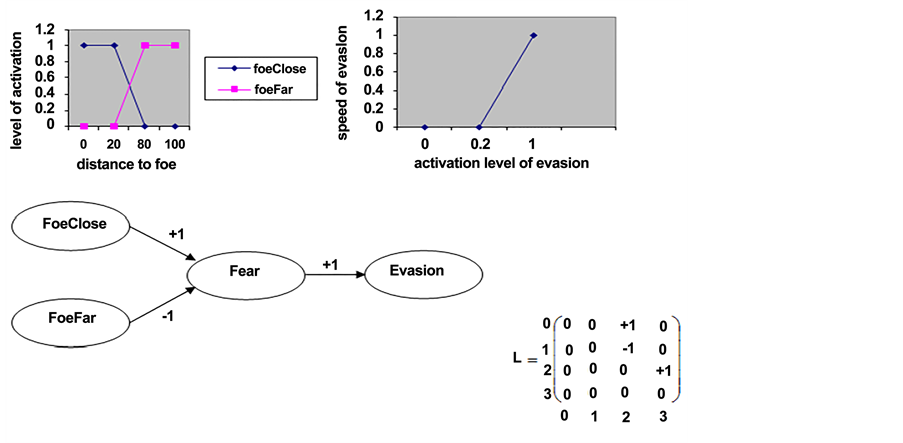
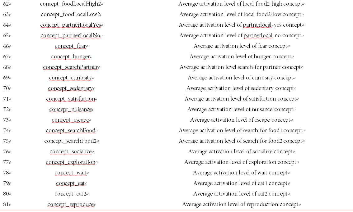
The virtual world of EcoSim is a torus environment of 1000 × 1000 discrete cells. Each cell contains an unlimited number of prey and predator individuals, but a limited amount of primary resources. The resource amount and spatial distribution varies dynamically in time [54] . Prey and predator individuals live in a world consisting of discrete cells. This model goes through separate time steps. During each time step, living organisms perform different actions based on their perception of their surrounding environment and of the other organisms that they are in interaction with. This, in consequence, influences the whole system. Prey and predator species coexist and they need efficient, evolvable behaviors to be able to survive and adapt to the evolving virtual world [51] . The behavior of each living organism is coded in its genome and implemented via a Fuzzy Cognitive Map (FCM) [55] . As such, individuals are able to perceive their environment using their FCM and then perform at any time step the behavior they perceive as the most beneficial. This means that at every time step, each individual will perform a unique action as determined by its behavioral model and its surrounding environment. The FCM of each agent, being coded in its genome, thus allows the evolution of the agent behavior through the simulation. As a result of utilizing such a complicated modelling approach, each individual in EcoSim can express different and divergent behavior [51] . Using FCM we were able to create a simulated ecological system called EcoSim to test sympatric spe- ciation. The FCMs consist of directed graphs containing nodes that represent concepts and the edges from one concept to another, which demonstrate the influences between concepts. The influence of the concepts in an FCM with n concepts can be represented in an n × n matrix. A positive weight associated with the edge eij corresponds to an excitation of the concept cj from the concept ci, whereas a negative weight is related to an inhibition (a zero value indicates that there is no influence of ci on cj). Individuals in EcoSim have three sets of concepts: Sensitive (distance of individual from food, predator etc.), Internal (such as fear, hunger etc.), and Motor (such as evasion of predators, eating, etc.). Sensitive concepts are set by mapping a perception out of an environmental observation. At initialization, the Sensitive concepts affect Internal concepts that in turn affect Motor concepts, but evolution can add edges between any concepts allowing some complex feedback loops to emerge. A number is associated with each concept, which is called the concept’s “activation level.” Activation levels are updated at each time step, using a concept’s current activation level and the weighted sum of other concepts’ activation levels affecting that concept, transformed by a non-linear function. The activation level of a Sensitive concept is computed by performing a “fuzzification” of the information an individual per- ceives from the environment. For an Internal or Motor concept, the activation level is computed by applying a de-fuzzification function on the weighted sum of the current activation level of all the concepts having an edge directed toward it. Finally, the action of an individual is selected based on the maximum value of the Motor concepts’ activation level. Activation levels of Motor concepts are used to determine the next action of the individual and its amplitude (See Tables A1-A4 in the Appendix).
For example a simple FCM regarding two Sensitive concepts (foeClose and foeFar), one Internal concept (fear) and one Motor concept (evasion) can have three influence edges: closeness to a foe excites fear, distance to a foe inhibits fear, and fear causes evasion (Figure 1). Fuzzification of concepts foeClose (nearness to the predator) and foeFar (distance from predator) provide the activation of the concepts depending on the distance of prey from a predator. De- fuzzification of the evasion concept provides the speed at which preys evade. Therefore, the FCMs are weighted graphs representing the causal relationship between Sensitive, Internal, and Motor nodes. The activation levels of the concepts of an individual are never reset during its life. Hence, the previous states of an individual participate in the computation of its current state. Therefore, an in- dividual has a memory of its own past and this will influence the individual’s future states. As the action undertaken by an individual at a given time step depends on the current activation level of the motor concepts, the global behavior of the
Figure 1. An FCM for detection of foe (predator) and decision to evade with its corresponding matrix (0 for “Foe close”, 1 for “Foe far”, 2 for “Fear” and 3 for “Evasion”) and the fuzzification and defuzzification functions [51] .
individual depends on a complex combination of the individual’s perception, the current internal states, and the past states it went through during its life [51] .
In EcoSim every individual possesses its own properties, which are mostly related to physical capabilities such as: age, minimum age for breeding, speed, vision distance, level of energy, and the amount of energy transmitted to the off- spring. Prey individuals obtain their required energy through the consumption of the available primary producer (grass) in the environment. Throughout the world, primary resource distribution is dynamic in terms of quantity and location. Predator individuals prey on herbivores to satisfy their energy needs. As a result of performing each action (eating, reproducing, etc.), each individual loses some amount of energy based on the type of action performed and the complexity of its behavioral model (the number of existing edges in its FCM). In this evolving system the process of producing a new individual occurs when two individuals that possess essential prerequisites for mating action (being in the same cell, both choosing to express reproduction action as their first priority among other actions, having the minimum age of reproduction, having the mi- nimum level of required energy, and being genetically close enough) perform a successful mating action. The produced offspring will inherit its parents’ genome combination with some mutations.
The notion of species is also implemented in this modeling system so that species will emerge from the evolving population of agents. Accordingly, “species” is defined in this model as a set of individuals with similar genomic charac- teristics, and the defined genome of a given species results from the average genomic characteristics of all its individual members. A species splits if the distance between the genomes of the two most dissimilar agents is greater than a predefined threshold. This is considered as speciation event [45] [51] . Consequently, the initial species is split into two sister species using a 2-mean clustering algorithm [56] . The resulting sister species contains individuals that show more intraspecific genetic similarity.
2.2. Modeling Sympatric Speciation Using EcoSim Model
This study focuses on the relationship between the first and the second trophic level, primary food resources (grass), and prey species to model resource-based diversification. As such, a second type of food resource has been added to the model to provide more than one food resource for prey individuals to feed on (see Figure A1, a and b in the Appendix).
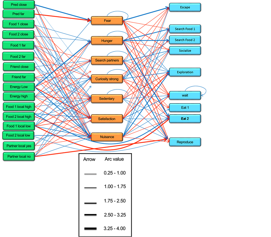
In one single resource version (original version of EcoSim), FCM maps of prey individuals contain four Sensitive and two Motor concepts that are directly related to the prey’s food consumption. These Sensitive concepts are: Food Close, Food Far, Food Local High, and Food Local Low. A Motor concept related to prey food consumption is Search For Food and Eat. Hunger, Search Partner, Curiosity, Sedentary, Satisfaction, and Nuisance are the Internal concepts in prey FCMs that are influenced by prey food consumption. In order to avoid any initial bias regarding the introduction of a new food resource to the system, the prey FCM is modified by adding four new Sensitive concepts of; Food Close 2, Food Far 2, Food Local High 2, and Food Local Low 2 as well as two new Motor concepts: Search For Food 2 and Eat 2 (Figure A2(a) in the Appendix changed to Figure A2(b) in the Appendix). New edges between Sensitive, Internal and Motor concepts in prey FCMs are also added. The complete FCM maps of prey individuals after adding the extra source of food is shown in Figure 2.
The new food resource added to the system possesses specific characteristics (Table 1) that we customized to create two different food resources that differ from each other in their probability of diffusion, speed of growth, and the amount of energy obtained from feeding on each food resource (the amount of energy transferred to a prey individual after eating one unit of each food resource). In general, each unit of Food 2 contains a higher amount of energy than that in one unit of Food 1. In other words, Food 2 tends to be more valuable in
Figure 2. The initial Prey FCM including concepts and edges for the dual resource version of the EcoSim (modified version of the original version of Ecosim). The width of each edge indicates its influence value. The color of an edge shows inhibitory (red) or excitatory (blue) effects.
Table 1. The main characteristics of food resources for the prey individuals.
terms of the amount of energy transmitted to prey consumers. However, Food 1 is more accessible as it grows faster and spreads throughout the world at a higher rate than Food 2. Introducing dissimilar food resources with different levels of availability and energy content to the simulated world creates the favorable conditions for the emergence of food consumption specialization in prey individuals (either getting specialized on more available food or food with higher energy content).
2.3. Indicators of the Occurrence of Sympatric Speciation
Bolnick and Fitzpatrick (2007) modified sympatric speciation requirements introduced by Coyne and Orr (2004) and defined four different basic criteria for the occurrence of sympatric speciation: firstly, species undergoing speciation must be sister species; secondly, there must be a complete reproductive isolation between these species; thirdly, there must be a complete (or extensive) geogra- phical overlap between these species; fourthly, the occurrence of allopatric/para- patric speciation must be highly improbable to be able to reject alternative hypotheses [1] [39] . However, it is difficult for empirical investigations to fulfill these requirements. Computational simulations on the other hand, provide complete control over a huge number of discrete factors and facilitate the development of models addressing the complex interactions between species that give rise to sympatric speciation. Modeling simulations take advantage of computational resources, and thereby enable us to closely monitor and investigate speciation events in a reasonable time period. Additionally, these modeling approaches facilitate the process of quantitative analysis of data. Considering the pragmatic application of the modeling approach in investigating the speciation process, we employed an IBM approach and followed the suggested requirements for the occurrence of sympatric speciation as defined by Bolnick and Fitzpatrick (2007) and defined four criteria (Table 2) that must be fulfilled in order to consider a speciation event as a “sympatric divergence”. As illustrated in Table 2, four dif- ferent methods were employed to test each criterion. This criteria and applied
Table 2. Sympatric speciation criteria and chosen strategy.
methods will be further described in the following subsections. As soon as one run was complete, a large amount of information about individuals and species (e.g. their actions, their breeding information, and all the information about their behavioral FCM model), as well as a complete set of information about their surrounding environment (e.g. individual’s geographic location and the food abundance distribution in the environment) were provided to analyze and evaluate the occurrence of sympatric speciation. The first filter selected the runs in which divergent eating behavior had occurred and species had expressed a significant preference for one specific type of food resource (either primary resource Type 1 or Type 2). This filter was tested following the protocol described in section 2.4. Observing preferential behavior for different types of food resources among different coexisting species is interpreted as the first indicator of the occurrence of sympatric speciation. The second step of the analysis process was evaluating the four selected criteria, which will be discussed in Section 2.5.
2.4. Species Categorizing Algorithm
Two different approaches (FCM-Clustering Approach and Action-Perception Clustering Approach) were applied to detect species expressing preferential behavior toward one specific food resource. Under the first approach, FCM-Clus- tering Approach, each species’ average behavioral model was analyzed. This means that the behavioral model (FCM) of every individual of each species was averaged to obtain the average FCM for each species. This value can be used to evaluate the extent of the preference expressed by each species for each type of food resource to identify a species’ category. Under the second approach, Action-Perception Clustering Approach, the action performed by individuals of each species was examined. In other words, the real actions performed by individuals and also individuals’ perceptions of their surrounding resources were taken into account to evaluate whether they had any preferential behavior toward one specific resource or not. These approaches are thoroughly described in the following subsections. Employing these approaches enabled us to categorize species into three different groups based on their preferences for different food resources: Group One, the species that were more likely to choose Food1 rather than Food 2; Group Two, the species that had a preference for in consuming Food 2; and Group Three, the species without any particular preference for either food resource that simply chose the closest available food resource.
2.4.1. FCM-Clustering Approach
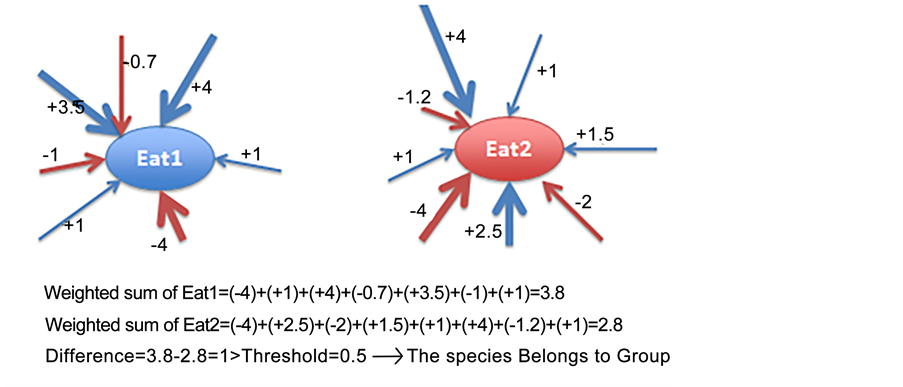
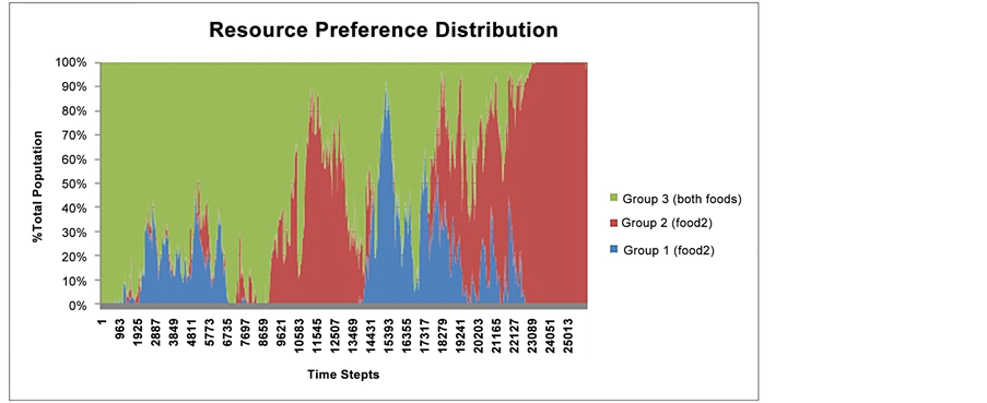
In order to determine if one species show preferential behavior toward a specific food resource or not, the weighted sum of all the edges that had influence on the Eat1 and Eat2 Motor concepts were separately calculated. Then, in order to categorize all existing species to three different groups, a threshold was defined to differentiate between the associated values of all edges coming to (influencing) the Eat1 and Eat2 Motor concepts. If the differences between the weighted sums assigned to Eat1 and Eat2 were smaller than 0.5, it was assumed that the species do not express any significant preference for either food resource and was assigned to Group Three (species with no preference). However, if the difference between the value associated to Eat1 and the value associated to Eat2 was greater than the threshold and the value of Eat1 was greater than the value of Eat2; then the species was assigned to Group One. In contrast, the species was categorized as Group Two under the opposite situation (see Figure A3 in the Appendix). After categorizing all existing species into three separate groups, the number of individuals belonging to each group was counted in each time step and (see Figure A4 in the Appendix).
2.4.2. Action-Perception Clustering Approach
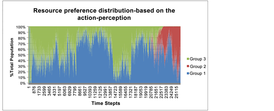
In the second approach, instead of using the FCM behavioral model (as employed in the first approach), species’ real behavior was applied as the main criteria for the classification of existing species into the three different groups (as discussed above). The rate of performed Eat 1 and Eat 2 actions by each species and the average perception for each species’ local food resource availability (Food 1 and 2) were taken into consideration. Five simple logical rules were applied to evaluate these two criteria (see Table A5 in the Appendix). The thresholds were chosen to ensure that the differences in behaviors and perceptions were significantly strong (see Figure A5 in the Appendix).
2.5. Verifying Required Criteria of Sympatric Speciation
2.5.1. First Criterion: Sister Species
The first criterion was identifying the sets of sister species that were specialized on different food resources. More precisely, it was necessary to consider any set of two species and determine whether they are sister species (each other closest relative) or not. This assessment had to be applied for all couples of species. Since every single individual of the prey and predator species were trackable through evolutionary time in our simulation study, we could simply construct the exact phylogenetic trees to determine the precise time of the occurrence of speciation. Thus, the phylogenetic trees were made to distinguish species with preference for one specific food resource. Consequently, this made it possible to categorize species on their phylogenetic tree in terms of their expressed preference for specific food resources. Based on the first criterion, three different categories obtained from the previous step were used to create and find a set of sister species, one specialized on Food 1 and the other specialized on Food 2.
Phylogenetic trees were computed using information such as parent species ID, offspring species ID, and the time steps where speciation events occurred. The life span of each species was applied to determine that species’ associated branch length in their phylogenetic tree. It should be noted that this program also had the related information obtained from the previous step regarding the species categorizing algorithm and their food preferences.
We needed to apply a method to visualize species that belonged to different categories (either specialized on Food 1 or Food 2), so that we could easily detect sister species with different food resource specializations. Therefore, a graphical editor for phylogenetic trees called Tree Graph [57] was applied. A truncated phylogenetic tree, rooting on a speciation event occurring at time step 17400, is presented in Figure 3. This represents a good example of a set of sister species that has met the first criterion. This set of sister species has lived for more than 400 time steps, that is why the length of their branches is so long. All other lines in this figure (shown in light blue and light red) indicate other species with shorter life spans.
Since the phylogenetic tree of each run was huge; containing thousands of species and all the speciation events, it was impossible to manually trace a set of sister species with different food preferences. As such, an algorithm was developed to distinguish all sets of sister species that met both of the following con- ditions: 1) one of them was specialized on Food 1, while the other one showed preference for Food 2; and 2) both were able to survive for at least 100 time steps.
The speciation event in EcoSim is determined by a two-means clustering method. Therefore, at any speciation event only two sister species emerge from a parent species. This means that in cases where there is potential for the emer-
Figure 3. A truncated phylogenetic tree centered on one species splitting in two sister species each expressing a preferential resource behavior for Food 1(blue bold) or Food 2 (red bold). The length of the branches are proportional to the number of time steps. A set of sister species presented in bold color (red and blue) is detectable in this figure, each indicating different food preferences (in each color). The branch in the color of bold blue belongs to Group 1 with preference for Food 1, whereas its sister species, the branch in the color of bold red, belongs to Group 2 specialized on Food 2.
gence of more than two sister species, it is possible to observe two consecutive speciation events within a very short period of time. In such cases, these species with such sequential speciation events are still considered as sister species as long as the difference between their originating time steps is less than five.
2.5.2. Second Criterion: Complete Reproductive Isolation
The second criterion was to ensure that there was a complete reproductive isolation between sister species that had already passed the first criterion. This criterion quantified the extent of reproductive isolation between sister species. The level of reproductive isolation between two sister species could be determined by measuring the number of occurrences of hybridization events. In other words, reproductive isolation level would be low if sister species frequently mate with each other and reproduced hybrid offspring. Therefore, measuring hybridization events was used to determine the level of reproductive isolation between sister species. The hybridization events were calculated as a ratio of all reproductive events that had occurred between all individual members of two sister species through evolutionary time. This ratio, then, measured intra- and inter-specific reproduction events. As the parents of each single individual were trackable in our simulation study, we only needed to go through all individual members of each sister species (that had already passed the first criterion) and calculate the ratio of intra-specific reproduction versus inter-specific reproduction occurring at each time step. The calculated hybridization ratio indicated that there were no occurrences of hybridization events between identified sister species from the first criterion.
2.5.3. Third Criterion: Overlapping Geographic Ranges
Spatial distribution of species was also examined to ensure that the two sister species occupied the same geographic habitat. In nature, dispersal ability of all individuals of one particular species determines the spatial extent of the habitat occupied by that species [1] . In studies focusing on resource distribution or host-plant mediated interactions, what matters is the dispersal ability of every single individual rather than the average of the population’s dispersal ability as a whole. To validate our third criteria, it was necessary to verify that speciation events occurred among individuals sharing the same geographical range. Thus, for all individuals belonging to either of two sister species (that had passed the first and the second criteria), the average distance was measured in number of cells for the first 200 time steps after the occurrence of a speciation event. Using this information we were able to calculate the minimum distance between the two closest individuals, the average distance of the 200 closest individuals, and the average distance between all the individuals in either sister species to determine the level of geographical closeness of species (Figure A6 in the Appendix).
Furthermore, to get an idea about the distance between the set of candidate sister species (that had already passed the first and the second criteria) compared to the distance between all other sister species in the simulation (that had not arisen through sympatric speciation), the above parameters (the minimum distance, the average distance of 200 closest, and the total average distance) were also measured between all other sister species. The measurement of the minimum and the average distance between all other sister species provided an estimation about the level of cohabitation. Thereby, we could define a threshold for the highest acceptable minimum and maximum distances between the individuals of the candidate sister species. These thresholds could be, ultimately, used to examine the third criterion. In other words, it is crucial to know: 1) what is the highest acceptable minimum distance, and 2) the maximum acceptable average total distance between the individuals of the sets of candidate sister species. According to the obtained results, the average geographic distance between individuals of the candidate sister species was significantly less than the average distances between all other sister species. Furthermore, in order to make sure that this important criterion (shared geographic habitat) was met, the statistical significance of the distances between every set of candidate sister species and all other sister species were also calculated through a T-Test. The result of this T-Test demonstrated that the distances between the candidate species (species that had already passed the first and the second criteria of sympatric speciation) were significantly differentiated from the distances between all other sister species. More importantly, the thresholds were estimated; 1) the minimum distance between the individuals of the sets of candidate sister species and the average distance between their closest 200 individuals must be zero (less than 0.01) during the first 50 time steps after the speciation. Also, 2) the total average distance between the sister species populations must be less than 13 during the same time (the first 50 time steps after the speciation).
In summary, as the third criterion, the distances between individuals of the candidate sister species (all couples of sister species, which had already successfully passed the two previous required sympatric speciation criteria) were measured.
When the distances for the individuals of the candidate sister species were equal or below the thresholds, this couple of sister species were considered to have passed the third required criterion, which implies that this particular couple of sister species occupies the same geographical habitat. More precisely, if the minimum distance between individuals of a couple of sister species and the average distance between their closest 200 individuals was 0 during the first 50 time steps after the speciation event, and also at the same time the total average distance between their populations was less than 13, this couple of sister species, then, fulfilled the third criterion.
2.5.4. Fourth Criterion: Rejecting Alternative Hypothesis (Allopatric/Parapatric Speciation)
In evolutionary modeling studies, it has been proven that sufficient evidence of the biogeography and evolutionary history of a sister species couple is required to validate the emergence of a new species through sympatric divergence, and reject the possibility of their resulting from allopatric or parapatric processes [1] , [39] . In this study, the biogeography of the two species in relation to one another was taken into account under the third criterion and the species’ phylogenetic lineage was examined through the first criterion.
The last required criterion was to reject the alternative hypothesis of allopatric and parapatric speciation, to attest that the two species supposing to have arisen through sympatric speciation have not undergone any geographic isolation. One of the advantages of this study is that it was possible to track all the phylogenetic and biogeographic information of every single individual within the populations. As a result of such a population tracking capability, sampling errors that are intrinsically unavoidable in experimental investigations were eliminated from this modeling study. This study enables us to follow the complete biogeographic and phylogenetic history of all species through evolutionary time. Furthermore, there were no physical barriers in EcoSim that could restrict individuals’ dispersal and movement to isolate the populations. As such, as soon as the first three criteria are met, the fourth criterion is also automatically met, and consequently, the possibility of the contribution of alternative hypothesis (allopatric/parapatric divergence) is contradicted.
2.6. Do Sympatric Species Share Some Common Patterns?
We applied machine learning techniques to find the shared patterns among sympatric species in the five runs with more than 10 instances of sympatric spe- ciation events. As such, three steps were followed (preparing the dataset, attri- bute selection, and classification), to analyze the results of these runs for further detailed information concerning the specific conditions leading to sympatric speciation.
2.6.1 Preparing and Preprocessing the Dataset
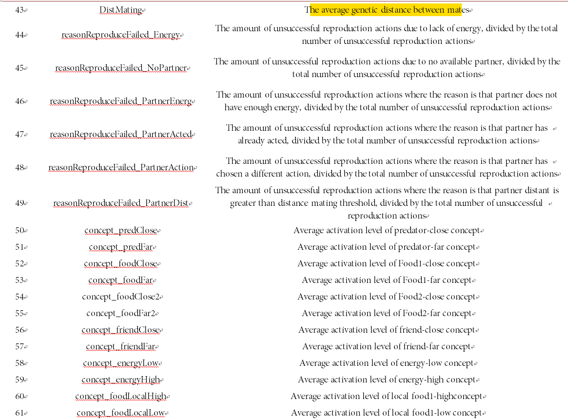
The results obtained from the five runs that had a high number of occurrences of sympatric speciation were used as the main dataset for applying the machine learning methods. In this dataset, sympatric species were labeled as positive instances, while other sister species at the same period of time were marked as negative instances. Initially, we included all attributes describing the species and their environment to create the initial dataset. These 81 attributes covered a broad range of information including general species information (such as population size of each species, their interbreeding ratio, and the amount of their energy transferred to an offspring), and behavioral specifications (such as the frequency of each action, and an individual’s perception of their environment).
Accordingly, five initial datasets were created from the five different runs. However, four of them were imbalanced, meaning that the number of positive samples was only one third of the number of negative samples. This can negatively affect the machine learning method’s ability to discover significant rules. One main approach to solve the imbalanced dataset problem is to either oversample the minority class or under sample the majority class [58] . Therefore, for those four imbalanced datasets, we applied the smote algorithm [59] to resample the minority class, which corresponded to our sympatric species (positive samples). After balancing the datasets, each had approximately 6000 to 7000 instances, where each instance contained the values of all the attributes describing one species (either in the positive or negative class).
2.6.2. Attribute Selection
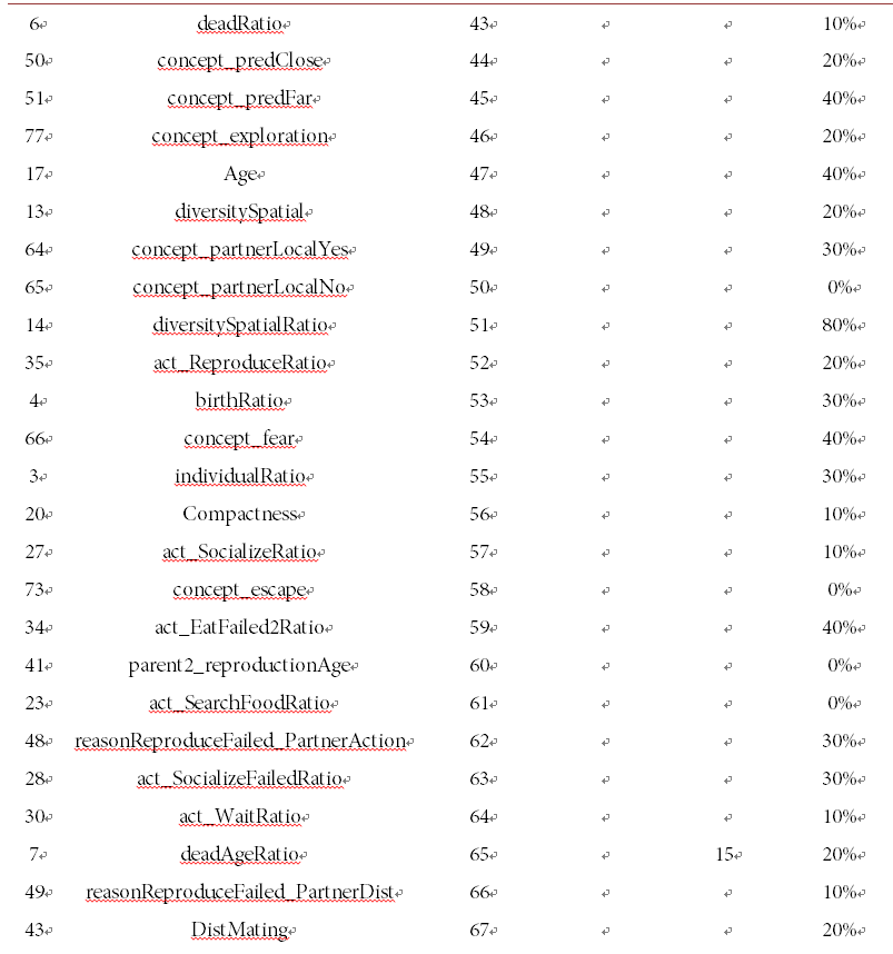
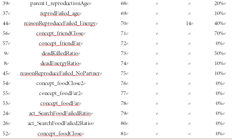
Each attribute describes one particular characteristic about a species, but not all attributes impact sympatric speciation. Thus, the most influential attributes were identified to classify the datasets in a way that will generate the most accurate results. Consequently, different attribute selection methods were used and their results were combined to select the attribute subset that most significantly discriminates between the two classes. We used the Info Gain Attribute Evaluator implemented in Weka [60] , combined with the Ranker search method and Cfs subset Evaluator in three different search methods (including Best First, Greedy Stepwise, and Genetic Search) [60] . Subsequently, all attributes were sorted by their corresponding scores, returned from the Ranker plus Info Gain Attribute Evaluator. The Ranker, combined with the Info Gain Attribute Evaluator, assigned a score to each attribute based on their relative importance for the learning process. The lower the rank of an attribute, the higher the importance. The Best First search method combined with the Cfs subset Evaluator only selected 8 attributes, corresponding to attributes already having a high importance based on the Ranker and Info Gain Evaluator combination. The Greedy Stepwise method combined with the Cfs subset Evaluator also returned a rank for the first 20 most important attributes. The Genetic Search method combined with the Cfs subset Evaluator was applied on a 10-fold cross-validation attribute selection basis. If an attribute was selected by evaluation of all 10 folds, a score of 100% was assigned to that attribute. Similarly, if an attribute was not selected by the evaluation of any fold, a score of 0% was assigned to that attribute. Accordingly, the attributes with the lowest score from all the attribute selection methods were removed. For this purpose, we removed attributes with a score of less than 30% from the Genetic Search and Cfs subset Evaluator, or with a rank higher than 40 on the Ranker and InfoGain attribute Evaluator. Since the removed attributes also had a low score in the GreedyStepwise + Csf method, they were not selected by the BestFirst + Csf method. As a result, the number of the attributes was reduced to 29. The list of these attributes is provided in the Appendix (Table A6 and Table A7).
2.6.3. Classification
1) Specific Rules Associated to Each Run
The J48 classifier in Weka [60] , the CRF combined rule extraction and feature elimination method in supervised Random Forest classification [61] , and the Random Forest classification combined with feature selection using hill climbing method [62] were applied to each dataset individually to find a fit method for classification.
First, each dataset was tested separately to extract the rules on each run. Then, all datasets were combined to identify the shared patterns among all runs. The J48 classification method returned a lower number of rules than the Random Forest methods. However, the Random Forest method provided the highest level of accuracy of classification, whereas the accuracy obtained with J48 was still reasonably high. Hence, we decided to use the J48 classifier to classify each dataset separately since it returned the lowest number of rules with a high accuracy.
J48 classifier was used with different attribute selection methods to find the minimum number of attributes, the minimum number of rules, and the highest accuracy. The classification started with the 29 attributes, selected using the attribute selection method (section 2.6.2). We pruned the decision tree by increasing the minimum number of instances per leave as this technique helped us to decrease the number of rules, which facilitated an explanation of the rules related to each class. A small part of each dataset was put aside to be utilized as a validation set. Hence, each dataset went through each step (pruning and removing attributes) separately. Starting with 29 attributes and 17 rules, it was possible to reduce down to 5 attributes and 11 rules. Consequently, the total accuracy declined from 96.26% to 86.79%, with the advantage of obtaining a reasonable number of short rules for interpretation. However, an accuracy greater than 86% is sufficient to capture the main properties and to provide a primary analysis of the conditions leading to sympatric speciation.
2) Generic Rules Valid for All Runs
The results of all the five runs were united to create a dataset to identify the shared patterns between all their sympatric species. The validation set consisted of 30% of the dataset put aside. Two methods of feature selection (the Info Gain Attribute Evaluator implemented at Weka [60] with the Ranker Search method, and the Cfs subset Evaluator with the Genetic Search method) were employed. Initially, 81 attributes were present in the dataset. First, the attributes were removed with scores less than 30% in the Cfs subset Evaluator with Genetic Search method or those with a rank higher than 30 in the Info Gain Attribute Evaluator with the Ranker search method were removed. As a result of the first step of feature selection, 25 attributes remained. Although a high number of attributes were removed, the total accuracy only dropped by approximately 1%, (from 97.25% [with 81 attributes] to 96.34% [with 25 attributes]). Accordingly, the number of rules decreased from 69 (with 81 attributes) to 56 (with 25 attributes).
In a second step, the J48 classification method was applied to the dataset with the remaining set of attributes. The tree pruning method was also utilized by increasing the minimum number of objects per leaf, which led to a decrease in the number of leaves and thereby, a decrease in the number of rules per class. The amount of pruning was chosen to significantly decrease the number of rules when keeping the total accuracy at a reasonable level.
The total accuracy marginally declined to 94.95% and the number of rules dropped to 42. These steps were repeated three more times and 13, 11, and 9 attributes were selected respectively after each step. The decision tree returned by the J48 classifier on all datasets combined together with 11 attributes and 20 rules is shown in the Appendix, Figure A7. In order to estimate how generic the discovered rules were, the classification process was repeated five more times. Each time the results of four out of the five datasets were united to use as the training set, while the results of the fifth dataset were exploited as the validation set. The attributes with the lowest score (as previously discussed) were removed step-by-step by applying the Info Gain Attribute Evaluator implemented in Weka [60] with the Ranker search method, and the Cfs subset Evaluator with Genetic Search method leading to the selection of 10 attributes. The J48 decision tree and Random Forest classification methods were also used in each experiment.
As expected, the total accuracy of the validation set in this experiment was much lower than the total accuracy of the 10-fold cross validation on the training set. This was due to the validation set having been created from the results of a different run. We observed that the Random Forest method strongly outperformed the J48 algorithm on the validation set and had a consistently higher accuracy on the training set.
2.7. Experimental Conditions
In order to detect the implications of resource partitioning on sympatric speciation, more than 50 runs of the dual resource version of the EcoSim with different initializations in terms of the foods’ specifications were executed on SHAR- CNET1. Each run was executed for about three months and provided 25000 time steps, which was long enough to observe the evolutionary behavior of the species. The process of evaluation of simulations for monitoring speciation phenomena was started at time steps 15,000 - 20,000, when populations had enough time to stabilize. All necessary data was stored individually for each simulation. Furthermore, 10 runs of the classic version of the EcoSim with only one food resource were also submitted as the control. The initial number of prey and predator in each run was 12,000 and 4900 respectively.
3. Results and Discussion
The Action-Perception Clustering approach (which categorized species into three groups based on the actual behavior of the individuals) provided a significantly higher number of sister species fulfilling the sympatric speciation requirements compared to the FCM-Clustering approach (which categorized species into three groups based on their FCM behavioral model). Under the FCM- Clustering approach, in each run we could only detect between 1 and 4 sets of sister species fulfilling criteria of sympatric speciation. Whereas, under the Action-Perception Clustering approach, each run contained between 11 and 53 sets of sympatric species (Table 3). The reason behind such a difference is that FCM-Clustering approach does not differentiate between the importance of the concepts influencing the Eat 1 and Eat 2 actions. In FCM some genes are more important than others as they are related to more important concepts. However,
Table 3. Initial number of sister species and the number of sister species that successfully met each of the required criterion in five runs with the most promising results of the occurrences of sympatric speciation.
FCM clustering approach does not comprise this fact when it is calculating the weighted sum of genes influencing Eat 1 and Eat 2. For instance, if there is a positive important edge and a negative less important edge influencing Eat 1 (both having the same value), they will cancel out each other. Although the positive one is more important than the negative one, as long as their absolute values are the same them will cancel each other. In consequence, some species specializing on one specific food resource may not have been found by simply examining their FCM through the FCM-Clustering algorithm. Out of the twenty total submitted test runs, five runs had more than ten instances of the occurrence of sympatric speciation, seven runs had one or two, and eight runs had not any instances of the occurrence of sympatric speciation. The three criteria were implemented on the five runs with the highest number of observed instances of sympatric speciation. Table 3 summarizes how speciation events were filtered step by step. As it can be observed, most of the speciation events have been filtered out after applying the first criterion, leaving the sister species that were specialized on different food resources and that had a life span greater than 100 time steps. Interestingly, all sets of sister species that passed the first criterion also successfully met the second required criterion (they were also found to be reproductively isolated). In some runs, a small number of sister species that had passed the first and the second criteria, failed to fulfill the third criterion since they lived too far from each other (Table 3).
The results of these five runs were used to create a dataset to investigate the probability of the occurrence of sympatric speciation. Although we observed very promising results in all runs, presenting all the results obtained from these five runs is beyond the scope of this study. The results presented here focus on run 4 since this run had the highest number of the occurrences of sympatric speciation. However, similar results were also observed for the other four runs.
3.1. Obtained Results from Run 4
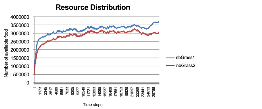
The total abundance of the different food resources is shown in Figure 4. In general, each simulation was allowed to run for about 25,000 time steps. It was necessary to give each run enough time to stabilize so that we were able to recognize the signs of speciation process around time steps 15,000 - 20,000. As mentioned earlier, Food 1 had a relatively higher probability of diffusion and grew faster than Food 2. On the other hand, Food 2 was less available but was a more valuable resource regarding the amount of energy transmitted to prey.
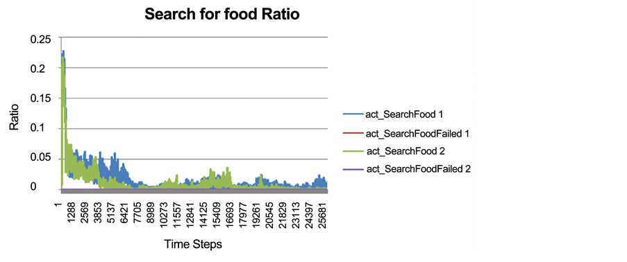
As described earlier, we were able to track the rate of any successful or failed action performed by prey individuals. The rate of successful or failed searching action for Food 1 and Food 2, (as a ratio to all performed actions by all prey individuals at each time step), is represented in Figure 5 for the two food resources. The very low level of a failed searching for food action shows that prey individuals in this run did not face any difficulties in finding either of the food resources.
Another important action that was investigated in this study was the eating action performed by prey individuals, feeding on two different food resources.
Figure 4. The total resource abundance of Food 1 (blue) and Food 2 (red) in different time steps.
Figure 5. The success or failure of searching for each food resource as a ratio to all actions performed by all prey individuals at every time step.
Figure 6 indicates the ratio of the number of successful or failed eating actions performed to the total number of all actions performed by all prey individuals at every time step.
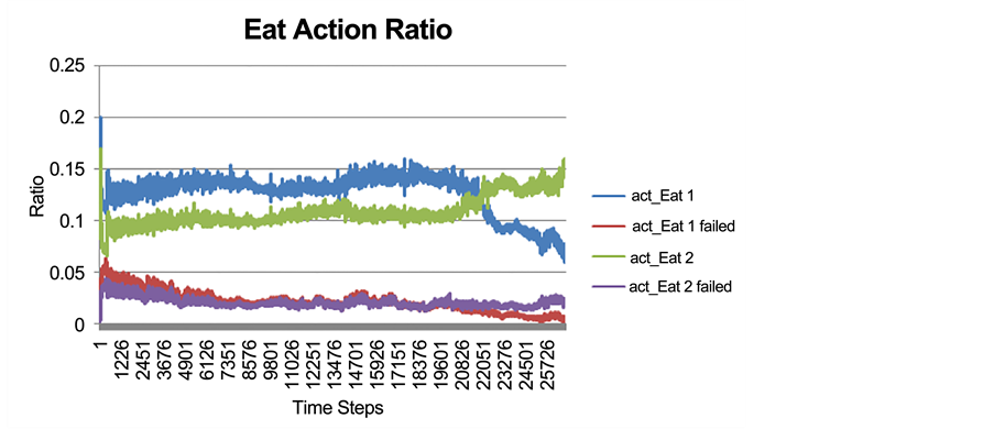
Initially, the rate of eating Food 1 is significantly higher than the rate of eating Food 2 (Figure 6). This is because at the beginning of the simulation, prey individuals were not specialized on any specific food resource and they simply fed on the most available food resource, which was Food 1 (Figure 4). Around time step 20,000, the rate of eating Food 2 suddenly built up (an increasing trend for Eat 2 action; Figure 6), and at the same time, an evident decreasing trend for the Eat 1 action occurred. As such, the ratio of these actions (Eat 1 and Eat 2) crossed each other near time step 22,000. Accordingly, from time step 22,000 the rate of the Eat 2 action was clearly higher than the rate of Eat 1 (Figure 6). Initially, there was no food consumption specialization and the majority of individuals consumed the more abundant food. However, after the occurrence of food specialization at time step 22,000, the consumption rate of Food 2 was greater than that of Food 1, although Food 2 was less available than Food 1. This means that, although there were higher costs and risks associated with the exploitation of Food 2 (such as “longer search time, vulnerability to variation in habitat abundance, etc.” [63] ), specialization evolved nevertheless.
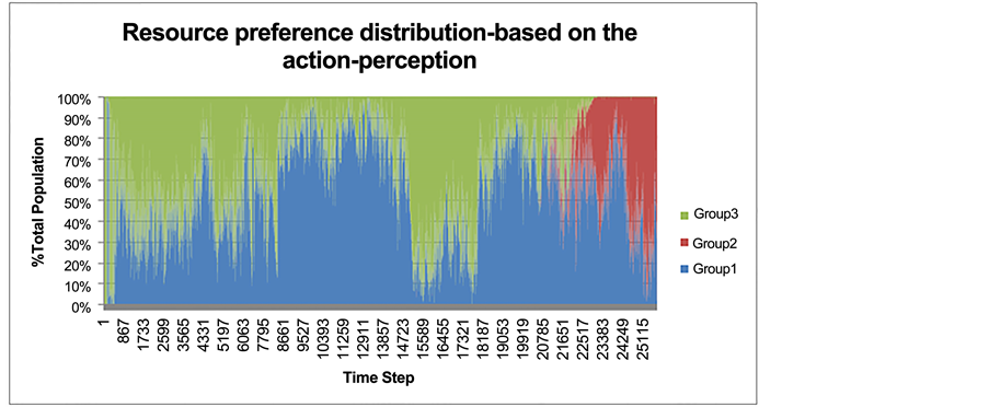
Resource preference distribution for Food 1, Food 2, and for both food resources is indicated in Figure 7. Starting near time step 22,000, a large proportion of the prey population specialized on Food 2 despite a higher availability of Food 1 (Figure 7). This explains the observed increase in the Eat 2 action after time step 22,000 (Figure 6). The obtained results on resource distribution demonstrated that while the difference between the availability levels of Food 1 and Food 2 follows a steady trend, starting from time step 22,000 this difference begins to increase, which reflects the effect of the preference for Food 2 (Figure 4).
3.2. Comparing Sympatric Sister Species with Non-Sympatric Sister Species
All sets of sympatric sister species (that had passed sympatric speciation requirements) were compared with all other sets of sister species (called non- sympatric sister species) in the simulations that failed to meet at least one sympatric speciation requirements. In other words, all sets of sister species (either sympatric or non-sympatric) with a minimum lifespan of 100 time steps in the duel resource version were compared with each other in terms of the hybridization ratio (between sister species) and the average geographical distance (between sister species) following the application of the same methods employed for testing the second and the third required criteria for the occurrence of sympatric speciation. Obtained results enabled us to draw a comparison between sympatric and non-sympatric sets of sister species in terms of the reproductive isolation level and the amount of geographical overlapping. This potentially illustrates the importance of required conditions for sympatric divergence.
As it is indicated in Table 3, there were five runs that each contained more
Figure 6. The successful and failed eating action on each type of food resource as a ratio to all actions performed by all prey individuals at every time step of the simulation.
Figure 7. Resource preference distribution for Food 1 (blue), Food 2 (red) or both re- sources (green). Each individual’s preference from the total prey population is calculated at every time step for the duration of the simulation.
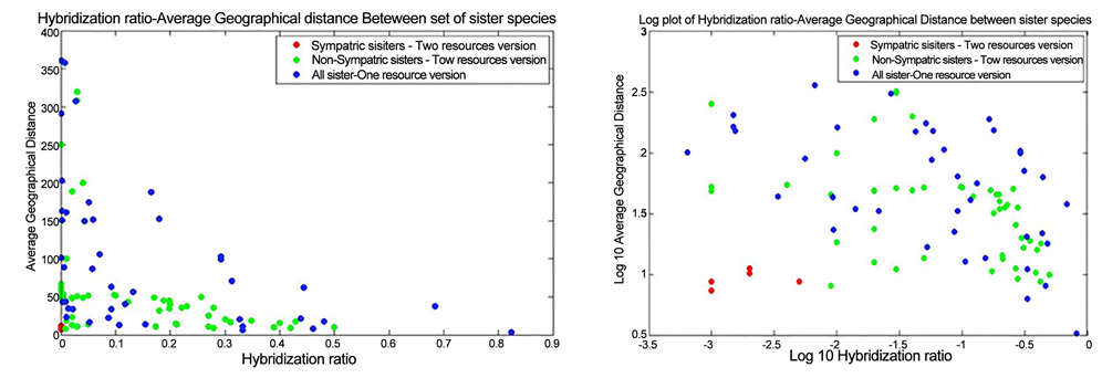
than ten candidates for the occurrence of sympatric speciation. These runs were used to calculate the hybridization ratio between the individual members of the sister species as well as the average geographical distance between their individuals. These distances were calculated for all sets of sister species with a minimum lifespan of 100 time steps (Figure 8(a) and Figure 8(b)).
According to observed results, the non-sympatric sister species were either not completely reproductively isolated or that they lived in a non-overlapping area. The differences between sympatric and non-sympatric sister species are even stronger when presented in the form of logarithmic plot (Figure 8(b)). For the occurrence of sympatric speciation, divergent species are required to inhabit the same habitat and share the same geographical range as their common ancestral species [7] [8] [9] . Therefore, it was expected to observe sympatric species exclusively in overlapping geographical habitats, in the absence of geographical isolation. More importantly, this study demonstrated how exploiting different resources could exert disruptive selective pressure. This process thereby induces the formation of barriers to gene flow (reproductive isolation) and consequently, the emergence of new sympatric species [37] [64] [65] [66] . This modeling study therefore indicates that sympatric speciation could result from assortative mating driven by differential resource use as a divergent selective pressure. In this study, we showed that ecological divergence in the form of diverse feeding preferences and differential foraging behavior could lead to reproductive isolation and thereby, the emergence of sympatric species. Similar results have been observed in natural populations. For instance, 11 different cichlid species all share the same ancestral species (tilapiines cichlid). Each of these species specializes on a particular food resource. Schliewen, Tautz, and Pääbo (1994) proved that these species have sympatrically diverged from their common ancestor species [67] . Furthermore, two species of three-spined sticklebacks have been verified to have arisen through sympatric speciation as a result of becoming specialized on different food resources [68] [69] [70] [71] [72] .
Moreover, all sets of sister species in the dual resource simulation that had a minimum lifespan of 100 time steps were compared with all sets of sister species with a lifespan of more than 100 time steps in the single resource simulation (control simulations). In order to illustrate the importance of the presence of two different food resources in sympatric divergence, a comparison was made between all sets of sister species from the dual and single resource simulations (Figure 9(a) and Figure 9(b)).
We couldn’t find any examples of sister species fulfilling sympatric speciation requirements in the single resource version runs, and species that met the required criteria are all from the dual resource simulations. Therefore, this model
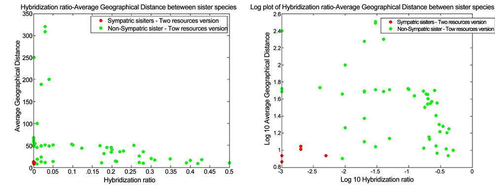
Figure 8. The scatter plot (a) and logarithmic plot (b) of the hybridization ratio and the average geographical distance between all individuals of sister species in the dual resource version of EcoSim. Red circles represent sympatric sister species, while green circles shows non-sympatric sister species. Sympatric sister species (red circles) are strongly clustered in the lower left part of the graph, whereas the non-sympatric sister species (green circles) are distributed along the two axes.
Figure 9. The scatter plot (a) and logarithmic plot (b) of the hybridization ratio and the average geographical distance of the sister species for the dual and single resource versions of the EcoSim. The blue circles represent all sets of sister species from the single resource version. The red and the green circles indicate sympatric and non-sympatric sister species respectively.
demonstrated that divergent foraging behavior could potentially result in reproductive isolation between sister species and eventually lead to sympatric speciation.
This study indicates how environmental variation in the case of diverse resource acquisition could play a very fundamental role as the main driver of divergent selection leading to the evolution of sympatric races. This observation supports previous claims regarding the crucial role of “ecologically-based divergent selection” [66] and divergent selection caused by environmental variances [22] in the evolution of sympatric species.
When one population is offered different choices of food resources, a proportion of the population may begin exclusively exploiting one particular resource, and this could initiate a barrier to gene flow between this part of the population and the main population. That is why natural selection is considered the most central factor in the emergence of new species [72] - [77] . Our observation is also consistent with studies that consider ecological interactions to have an extremely important role among living organisms as a source of divergent selection in sympatric speciation [38] [66] .
These results therefore support the main hypothesis of this modeling investigation regarding the importance of the presence of multiple resources in sympatric divergence. It has been established that different local environments could result in the evolution of distinct characteristics, and consequently lead to the emergence of sympatric species [78] . In fact, specialization on different food resources exerts varying extents of ecological forces that lead to the emergence of prezygotic isolation through natural selection [38] . African Finches (Pyrenestesostrinus), Salamander (Ambystomatigrinum), and Arctic Charr (Salvelinusalpinus) are typical examples of vertebrate species that have indicated discrete intraspecific morphs, varying in food and habitat preference, and have evolved to exploit diverse resources [79] . Indo-pacific goby and its sister species are another example that could clearly illustrate the fundamental role of foraging behavior in a lineage-splitting event. Scientists have identified a brand new species of goby within the range of the Indo-pacific goby species’ habitat that is in fact its sister species and is exclusively specialized on a distinct coral host [80] .
Reproductive isolation or the emergence of barrier to gene flow might occur either before or after the formation of a hybrid zygote (respectively called the prezygotic or postzygotic isolating mechanisms) [7] . It is believed that compared to postzygotic (e.g. hybrid sterility), a prezygotic isolation (e.g. behavioral mating preference), which is considered an “earlier-evolving barrier to gene flow”, plays a more significant role in the speciation process [81] .
3.3. The Obtained Results of Machine Learning Techniques and Shared Patterns among Sympatric Species
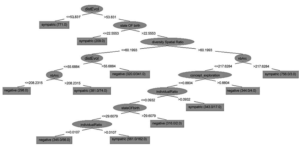
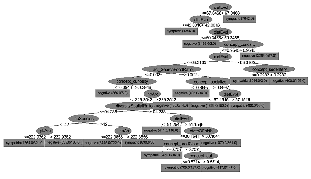
An example of the decision tree generated for Run #2 is presented in Figure 10. As is noticeable in this example, sympatric speciation has occurred at low values of disEvol (the average genetic distance between the initial reference genome and the current genomes). The evolutionary distance (disEvol) is always increasing with time; therefore, a low value of disEvol represents the beginning of the data measurement near time step 20,000 when the food specialization process was about to begin. This means that sympatric speciation has occurred at the beginning of the food specialization process, when an initial specialization on different food resources was developing (Figure 10). The same pattern was observed in all other generated decision trees.
The rules generated by the decision tree for this run (Run#2) demonstrated that sympatric speciation had mostly occurred at the beginning of the food specialization (disEvol low) except when the species’ spatial distribution was large
Figure 10. Decision tree corresponding to Run #2 with 11 rules.
(diversity Spatial Ratio high). Under this circumstance, two different criteria were needed for the occurrence of sympatric speciation. First, sister species required a high number of genes in their genomes (nArc high). This is intuitive since more genetic diversity results in a higher mutations rate and thereby, drives a faster genetic divergence. Kawecki (1996, 1997) illustrated the importance of the accumulation of beneficial or deleterious mutations corresponding to habitat and resource exploitation. His research showed that disruptive selection through habitat-specific deleterious or beneficial mutations could result in sympatric speciation [63] [82] . It has been proven that the expression of a habitat preference behavior could be spread among the gene pool of an initially random dispersing population via beneficial [34] [36] [82] [83] or deleterious [63] mutations, when selective pressure favors habitat preference over generalism. This eventually leads to the evolution of polymorphism and sympatric divergence.
The second condition occurred when species contained a large number of individuals (individual Ratio high). This means that species with a larger population size (compared to the whole populations of all species living in the simulation’s world) had a higher chance of experiencing sympatric speciation. This observation supports the claim that the extent of genetic diversity builds up with an increasing effective population size [84] . Additionally, as mentioned above, such increased genetic variability leads to a more diverse ancestral gene pool and thereby, increases the chance that sympatric speciation will occur [63] [82] .
The averages of the classification results of the five experiments are also summarized in Table 4, giving the TP; the True Positive rate and the AUC; the Area Under the Receiver Operating Characteristics (ROC) Curve. ROC curves are curves that are exploited in machine learning and data mining investigations with the purpose of both organizing classifiers and obtaining a clear visualization of their performance [85] . “An ROC curve is a two-dimensional depiction of classifier performance” [85] . In order to draw a comparison between classifiers, ROC performance needs to be decreased to “one single scaler representing expected performance” [85] . The AUC method is frequently used to measure the area under the ROC curve [86] [87] . The AUC varies between 0 and 1, but a realistic classifier should not have an AUC less than 0.5 [85] . Applying the Random Forest method we can predict the occurrence of sympatric speciation on the training set with an average accuracy of 99.97%. Furthermore, the unseen validation sets from different runsobtained an average accuracy of 82.22%, which is
Table 4. The average results of five experiments of classification using J48 and Random Forest classification methods.For each experiment four out of five datasets were used as the training set, while the fifth dataset was used as the validation set.
considered a high accuracy, indicating that our method was able to discover very generic rules that have the potential to reflect some meaningful properties of sympatric speciation.
4. Conclusions
There is still long-standing controversy surrounding sympatric speciation. Despite a general agreement on the theoretical plausibility of the incidence of sympatric divergence in nature, the extent that sympatric speciation may contribute to biodiversity and its root causes are still unknown today.
It is believed that strong disruptive selective pressure exerted by both competition for and specialization on resources could play a significant role in sympatric divergence [1] [10] - [15] [20] . However, the importance of ecological interactions and consequent disruptive selection in sympatric speciation still needs further investigation.
In order to obtain a better understanding of the evolutionary impact of the arrival of a new species, and to investigate speciation and lineage-splitting events, it is necessary to have access to a species’ complete evolutionary history including thousands of generations leading to a speciation event [1] [9] [39] . Achieving such insight is challenging by means of experimental and field investigations due to the unreasonable time investment for such a field study. Therefore, in this study we utilized the ability of an individual-based modeling approach in tracking the evolutionary paths of species [41] .
According to the results of this investigation, prey individuals mainly fed on the more abundant resource (Food 1) at the beginning of the simulations, before they had adapted to efficiently exploiting each specific resource. However, after the evolution of specialization around time step 22,000, consumption of Food 2 exceeded that of Food 1 in spite of the fact that Food 1 was more available and prey individuals encountered this resource more frequently. The main focus of this study was to investigate whether and under which circumstances the selective pressures acting on foraging behaviors could sympatrically diverge lineages. Four different criteria suggested by Bolnick and Fitzpatrick (2007) were employed, and we detected an indicator of the occurrence of sympatric speciation in 12 of our runs out of 20. After testing these four required criteria to identify sympatric speciation in the dual resource simulations, sympatric and non-sym- patric sister species with a minimum lifespan of 100 time steps were compared in terms of their level of reproductive isolation and amount of geographical overlapping (between individual members of the sister species). This was employed to obtain a better understanding of the underlying causes of sympatric divergence. As it was expected, the instances of sympatric species were exclusively observed among sister species that shared the same geographical ranges. Moreover, this comparison revealed the significant role of reproductive isolation and assortative mating caused by disruptive selection pressure exerted by the exploitation of different resources in sympatric speciation [37] [64] [65] [66] . Comparing the results obtained from the dual resource simulations with the single resource control simulations highlighted the importance of divergent foraging behavior and consequent reproductive isolation in sympatric divergence. This is because there were no incidences of sympatric speciation in the single resource control simulations. This result is consistent with previous observations regarding the role of ecologically-based divergent selection and ecological interactions among living organisms in sympatric speciation [22] [38] [66] [72] - [77] . The results of this study support the theoretical claim that reproductive isolation caused by assortative mating as a result of divergent selection pressures inflicted by resource differentiation could potentially lead to sympatric speciation [39] [88] [89] .
Our unique modeling approach does not simply assume that individuals are involved in foraging and mating activities; it also comprises all other possible considerations, which might play an important role from evolutionary perspective. Applying this complex modeling approach we highlighted significant indicators of behavioral modifications caused by preferential resource use. Finally, when employing the several machine learning techniques, explicit rules were extracted to gain more information regarding the most essential patterns that lead to sympatric speciation. According to our acquired rules, the majority of incidences of sympatric divergence occurred at the beginning of the process of resource specialization. However, if species had a high spatial distribution, they needed to fulfill two different conditions to diverge sympatrically: 1) high genetic diversity, and 2) large population size. This means that the probability of sympatric divergence was higher if a population had a more diverse gene pool and also a higher number of individual members. It has been empirically verified that genetic conditions and ecological conditions are the key components that facilitate the occurrence of sympatric speciation [1] [21] . In the case of specialized resource use, genotype × environment interaction is the leading contributor to sympatric divergence [21] . Our modeling study indicated the crucial role of these factors in the occurrence of sympatric speciation and stressed the importance of genetic diversity and population size.
One of the difficulties of empirical investigations of sympatric speciation is that it is almost impossible to reach a solid conclusion about ancestor species, as it is difficult to gain access to the genetic conditions of the initial population (ancestral species) prior to a divergence event [90] [91] . In most empirical studies addressing speciation, a speciation event has either completed and species have completely diverged, or it is currently happening. On the other hand, it has been claimed that the most accurate estimations about the initial conditions leading to sympatric speciation could be obtained from lineages that are beginning the divergence process [92] . Since modeling approaches provide us with an ideal opportunity to monitor speciation events at early stages of divergence, these tools are considered one of the strongest candidate approaches to achieve an accurate prediction of the initial requirements for speciation [92] . Our modeling investigation strongly supports this claim and illustrates the importance of an early stage of resource specialization in the occurrence of sympatric speciation. This modeling study provided us a golden opportunity to follow the speciation process since its initiation stage, something that is impossible in nature. The valuable obtained results of this study shed light on the central role of sympatric speciation in evolutionary ecology. More importantly, this study enabled us to overcome one the greatest obstacle in investigation sympatric speciation, which is having access to the evolutionary history and biogeography of sister species undergoing divergence process since it is almost impossible to have access to such information in the real world.
From a biological point of view, however, this modeling study has some limitations in spite of its major contributions to this field of study. EcoSim is intrinsically designed to address broad ecological and biological questions and it is not able to exclusively model a specific ecological system or a distinct species with high specificity.
Furthermore, the extent of the complexity of interactions and behavioral patterns among components of a real ecosystem is much greater than that modeled in this simulated ecological system. More importantly, it has been demonstrated that phenotypic adaptation is a key in sympatric speciation caused by specialized resource use. For example, it has been verified that a population with different food preferences than its original population gradually evolves a dissimilar phenotypic structure [93] [94] . This is evident in the evolution of phenotypic polymorphisms in amphibians, in terms of teeth length and mouth size in order to increase foraging efficiency [79] ; the evolution of different morphs in benthic and limnetic species of stickleback fish [68] [69] [70] [71] [72] ; and the evolution of divergent shape and size in Darwin’s finches to exploit different resources [93] [94] . Because this modeling study did not include any particular phenotypic traits, we did not evaluate the role phenotypic adaptation and adaptive radiation may have in sympatric divergence caused by resource specialization. This would therefore be a beneficial area for future work. In the current study, we simply evaluated runs with sympatric species; however, it would be valuable in future work to also involve runs without sympatric divergence. This may allow us to obtain a greater understanding of the environmental and behavioral differences between these runs that might have led to sympatric speciation.
Cite this paper
Pour, M.K., Bandehbahman, S., Gras, R. and Cristescu, M.E. (2017) An Individual-Based Modeling Approach to Investigate Sympatric Speciation via Specialized Resource Usage. Open Jour- nal of Ecology, 7, 222-269. https://doi.org/10.4236/oje.2017.73017
References
- 1. Bolnick, D.I. and Fitzpatrick, B.M. (2007) Sympatric Speciation: Models and Empirical Evidence. Annual Review of Ecology, Evolution, and Systematics, 38, 459-487.
https://doi.org/10.1146/annurev.ecolsys.38.091206.095804 - 2. Mayr, E. (1963) Animal Species and Evolution. Belknap Press of Harvard University Press, Cambridge.
https://doi.org/10.4159/harvard.9780674865327 - 3. Rice, W.R. and Hostert, E.E. (1993) Laboratory Experiments on Speciation: What Have We Learned in 40 Years? Evolution (N.Y.), 47, 1637-1653.
https://doi.org/10.2307/2410209 - 4. Coyne, J.A. (1992) Genetics and Speciation. Nature, 355, 511-515.
https://doi.org/10.1038/355511a0 - 5. Bank, C., Bürger, R. and Hermisson, J. (2012) The Limits to Parapatric Speciation: Dobzhansky-Muller Incompatibilities in a Continent-Island Model. Genetics, 191, 845-863.
https://doi.org/10.1534/genetics.111.137513 - 6. Fisher, R.A. (1958) The Genetical Theory of Natural Selection. 2nd Edition, Dover.
- 7. Ridley, M. (2004) Evolution. 3rd Edition, Blackwell Pub., Oxford.
- 8. Coyne, J.A. (2007) Sympatric Speciation. Current Biology, 17, R787-R788.
https://doi.org/10.1016/j.cub.2007.06.056 - 9. Berlocher, S.H. and Feder, J.L. (2002) Sympatric Speciation in Phytophagous Insects: Moving beyond Controversy? Annual Review of Entomology, 47, 773-815.
https://doi.org/10.1146/annurev.ento.47.091201.145312 - 10. Kirkpatrick, M. and Ravigné, V. (2002) Speciation by Natural and Sexual Selection: Models and Experiments. The American Naturalist, 159, S22-S35.
https://doi.org/10.1086/338370 - 11. Roughgarden, J. (1972) Evolution of Niche Width. The American Naturalist, 106, 683-718.
https://doi.org/10.1086/282807 - 12. Pfennig, D.W. and Pfennig, K.S. (2010) Character Displacement and the Origins of Diversity. The American Naturalist, 176, S26.
- 13. Bolnick, D.I. and Smith, T. (2004) Can Intraspecific Competition Drive Disruptive Selection? An Experimental Test in Natural Populations of Sticklebacks. Evolution (N.Y.), 58, 608-618.
https://doi.org/10.1111/j.0014-3820.2004.tb01683.x - 14. Wilson, D.S. and Turelli, M. (1986) Stable Underdominance and the Evolutionary Invasion of Empty Niches. The American Naturalist, 127, 835-850.
https://doi.org/10.1086/284528 - 15. Martin, R.A. and Pfennig, D.W. (2009) Disruptive Selection in Natural Populations: the Roles of Ecological Specialization and Resource Competition. The American Naturalist, 174, 268-281.
https://doi.org/10.1086/600090 - 16. Hendry, A.P., Huber, S.K., De Leon, L.F., Herrel, A. and Podos, J. (2009) Disruptive Selection in a Bimodal Population of Darwin’s Finches. Proceedings of the Royal Society of London. Series B, 276, 753-759.
https://doi.org/10.1098/rspb.2008.1321 - 17. Schluter, D. and Grant, P.R. (1984) Determinants of Morphological Patterns in Communities of Darwin’s Finches. The American Naturalist, 123, 175-196.
https://doi.org/10.1086/284196 - 18. van Doorn, G.S., Edelaar, P. and Weissing, F.J. (2009) On the Origin of Species by Natural and Sexual Selection. Science, 326, 1704-1707.
- 19. Maan, M.E. and Seehausen, O. (2011) Ecology, Sexual Selection and Speciation. Ecology Letters, 14, 591-602.
https://doi.org/10.1111/j.1461-0248.2011.01606.x - 20. Thibert-Plante, X. and Hendry, A.P. (2011) Factors Influencing Progress toward Sympatric Speciation. Journal of Evolutionary Biology, 24, 2186-219.
- 21. Via, S. (2001) Sympatric Speciation in Animals: The Ugly Duckling Grows up. Trends in Ecology & Evolution, 16, 381-390.
https://doi.org/10.1016/S0169-5347(01)02188-7 - 22. Schluter, D. (2000) The Ecology of Adaptive Radiation. Oxford University Press.
- 23. Larsen, C.S. and Repcheck, J. (2008) Our Origins: Discovering Physical Anthropology. WW Norton & Company.
- 24. Feder, J.L. and Filchak, K.E. (1999) It’s about Time: The Evidence for Host Plant-Mediated Selection in the Apple maggot Fly, Rhagoletis pomonella, and Its Implications for Fitness Trade-Offs in Phytophagous Insects. Proceedings of the 10th International Symposium on Insect-Plant Relationships, 56, 211-225.
https://doi.org/10.1007/978-94-017-1890-5_27 - 25. Linn, C., Feder, J.L., Nojima, S., Dambroski, H.R., Berlocher, S.H. and Roelofs, W. (2003) Fruit Odor Discrimination and Sympatric Host Race Formation in Rhagoletis. Proceedings of the National Academy of Sciences, 100, 11490-11493.
https://doi.org/10.1073/pnas.1635049100 - 26. Wood, T.K. and Keese, M.C. (1990) Host-Plant-Induced Assortative Mating in Enchenopa treehoppers. Evolution (N.Y.), 44, 619-628.
https://doi.org/10.2307/2409439 - 27. Prowell, D.P., McMichael, M. and Silvain, J.-F. (2004) Multilocus Genetic Analysis of Host Use, Introgression, and Speciation in Host Strains of Fall Armyworm (Lepidoptera: Noctuidae). Annals of the Entomological Society of America, 97, 1034-1044.
https://doi.org/10.1603/0013-8746(2004)097[1034:MGAOHU]2.0.CO;2 - 28. Sezer, M. and Butlin, R.K. (1998) The Genetic Basis of Host Plant Adaptation in the Brown Planthopper (Nilaparvata lugens). Heredity (Edinb), 80, 499-508.
https://doi.org/10.1046/j.1365-2540.1998.00316.x - 29. Claridge, M.F., Dawah, H.A. and Wilson, M.R. (1997) Species: The Units of Biodiversity. Chapman & Hall Ltd.
- 30. Berlocher, S.H. (1999) Host Race or Species? Allozyme Characterization of the ‘Flowering Dogwood Fly’, a Member of the Rhagoletis pomonella Complex. Heredity (Edinb), 83, 652-662.
https://doi.org/10.1046/j.1365-2540.1999.00591.x - 31. Sorenson, M.D., Sefc, K.M. and Payne, R.B. (2003) Speciation by Host Switch in Brood Parasitic Indigobirds. Nature, 424, 928-931.
https://doi.org/10.1038/nature01863 - 32. Jiang, T., Feng, J., Sun, K. and Wang, J. (2008) Coexistence of Two Sympatric and Morphologically Similar Bat Species Rhinolophus affinis and Rhinolophus pearsoni. Progress in Natural Science, 18, 523-532.
https://doi.org/10.1016/j.pnsc.2007.12.005 - 33. Darwin, C. (1859) On the Origin of Species. John Murray, London.
- 34. Smith, J.M. (1966) Sympatric Speciation. The American Naturalist, 100, 637-650.
https://doi.org/10.1086/282457 - 35. Rice, W.R. (1984) Disruptive Selection on Habitat Preference and the Evolution of Reproductive Isolation: A Simulation Study. Evolution (N.Y.), 1251-1260.
- 36. Rice, W.R. (1987) Speciation via Habitat Specialization: The Evolution of Reproductive Isolation as a Correlated Character. Evolutionary Ecology, 1, 301-314.
https://doi.org/10.1007/BF02071555 - 37. Rice, W.R. and Salt, G.W. (1990) The Evolution of Reproductive Isolation as a Correlated Character under Sympatric Conditions: Experimental Evidence. Evolution (N.Y), 44, 1140-1152.
https://doi.org/10.2307/2409278 - 38. Turelli, M., Barton, N.H. and Coyne, J.A. (2001) Theory and Speciation. Trends in Ecology & Evolution, 16, 330-343.
https://doi.org/10.1016/S0169-5347(01)02177-2 - 39. Coyne, J.A. and Orr, H.A. (2004) Speciation. Sinauer Associates Sunderland, 37.
- 40. Gavrilets, S. (2004) Fitness Landscapes and the Origin of Species (MPB-41). Princeton University Press Princeton.
- 41. Grimm, V. and Railsback, S.F. (2013) Individual-Based Modeling and Ecology. Princeton University Press, Princeton.
- 42. Thibert-Plant, X. and Hendry, A.P. (2009) Five Questions on Ecological Speciation Addressed with Individual-Based Simulations. Journal of Molecular Biology, 22, 109-123.
https://doi.org/10.1111/j.1420-9101.2008.01627.x - 43. Labonne, J. and Hendry, A.P. (2010) Natural and Sexual Selection Giveth and Taketh away Reproductive Barriers: Models of Population Divergence in Guppies. The American Naturalist, 176, 26-39.
https://doi.org/10.1086/652992 - 44. Mashayekhi, M. and Gras, R. (2012) Investigating the Effect of Spatial Distribution and Spatiotemporal Information on Speciation Using Individual-Based Ecosystem Simulation. J. Comput., 2.
- 45. Gras, R., Golestani, A., Hendry, A.P. and Cristescu, M.E. (2015) Speciation without Pre-Defined Fitness Functions. PLoS ONE, 10, e0137838.
- 46. Golestani, A., Gras, R. and Cristescu, M. (2012) Speciation with Gene Flow in a Heterogeneous Virtual World: Can Physical Obstacles Accelerate Speciation? Proceedings of the Royal Society B: Biological Sciences, 279, 3055-3064.
- 47. Lu, G. and Bernatchez, L. (1999) Correlated Trophic Specialization and Genetic Divergence in Sympatric Lake Whitefish Ecotypes (Coregonus clupeaformis): Support for the Ecological Speciation Hypothesis. Evolution, 53, 1491-1505.
- 48. Dieckmann, U. and Doebeli, M. (1999) On the Origin of Species by Sympatric Spe-ciation. Nature, 400, 354-357.
https://doi.org/10.1038/22521 - 49. Hatfield, T. and Schluter, D. (1999) Ecological Speciation in Sticklebacks: Environment-Dependent Hybrid Fitness. Evolution, 53, 866-873.
https://doi.org/10.2307/2640726 - 50. Griffith, D. (1996) The Ecology of Resource Polymorphism in Vertebrates. Trends in Ecology & Evolution, 11, 25-26.
- 51. Gras, R., Devaurs, D., Wozniak, A. and Aspinall, A. (2009) An Individual-Based Evolving Predator-Prey Ecosystem Simulation Using a Fuzzy Cognitive Map as the Behavior Model. Artificial Life, 15, 423-463.
https://doi.org/10.1162/artl.2009.Gras.012 - 52. Mashayekhi, M., Golestani, A., Farahani, Y.M.F. and Gras, R. (2014) An Enhanced Artificial Ecosystem: Investigating Emergence of Ecological Niches. Artificial Life, 14, 693-700.
- 53. Khater, M., Murariu, D. and Gras, R. (2014) Contemporary Evolution and Genetic Change of Prey as a Response to Predator Removal. Ecological Informatics, 22, 13-22.
https://doi.org/10.1016/j.ecoinf.2014.02.005 - 54. Golestani, A. and Gras, R. (2011) Multifractal Phenomena in EcoSim, a Large Scale Individual-Based Ecosystem Simulation. International Conference on Artificial Intelligence, Las Vegas, 18-21 July 2011, 991-999.
- 55. Kosko, B. (1986) Fuzzy Cognitive Maps. International Journal of Man-Machine Stu-dies, 24, 65-75.
https://doi.org/10.1016/S0020-7373(86)80040-2 - 56. Aspinall, A. and Gras, R. (2010) K-Means Clustering as a Speciation Mechanism within an Individual-Based Evolving Predator-Prey Ecosystem Simulation. Active Media Technology, Toronto, 28-30 August 2010, 318-329.
- 57. Stöver, B.C. and Müller, K.F. (2010) TreeGraph 2: Combining and Visualizing Evidence from Different Phylogenetic Analyses. BMC Bioinformatics, 11, 7.
https://doi.org/10.1186/1471-2105-11-7 - 58. He, H. and Garcia, E.A. (2009) Learning from Imbalanced Data. IEEE Transactions on Knowledge and Data Engineering, 21, 1263-1284.
https://doi.org/10.1109/TKDE.2008.239 - 59. Chawla, N. and Bowyer, K. (2002) SMOTE: Synthetic Minority Over-Sampling Technique Nitesh. Journal of Artificial Intelligence Research, 16, 321-357.
- 60. Hall, M., Frank, E., Holmes, G., Pfahringer, B., Reutemann, P. and I.H. (2009) The WEKA Data Mining Software: An Update. ACM SIGKDD Explorations Newsletter, 11, 10-18.
- 61. Liu, S., Patel, R.Y., Daga, P.R., Liu, H., Fu, G., Doerksen, R.J., Chen, Y. and Wilkins, D.E. (2012) Combined Rule Extraction and Feature Elimination in Supervised Classification. IEEE Transactions on NanoBioscience, 11, 228-236.
https://doi.org/10.1109/TNB.2012.2213264 - 62. Mashayekhi, M. and Gras, R. (2015) Rule Extraction from Random Forest: The RF + HC Methods. Advances in Artificial Intelligence, Canberra, 30 November-4 December 2015, 223-237.
- 63. Kawecki, T.J. (1997) Sympatric Speciation via Habitat Specialization Driven by Deleterious Mutations. Evolution, 51, 1751-1763.
https://doi.org/10.2307/2410998 - 64. Kautt, A.F., Machado-Schiaffino, G. and Meyer, A. (2016) Multispecies Outcomes of Sympatric Speciation after Admixture with the Source Population in Two Radiations of Nicaraguan Crater Lake Cichlids. PLOS Genetics, 12, e1006157.
https://doi.org/10.1371/journal.pgen.1006157 - 65. Schluter, D. (2001) Ecology and the Origin of Species. Trends in Ecology & Evolution, 16, 372-380.
https://doi.org/10.1016/S0169-5347(01)02198-X - 66. Rundle, H.D. and Nosil, P. (2005) Ecological Speciation. Ecology Letters, 8, 336-352. https://doi.org/10.1111/j.1461-0248.2004.00715.x
- 67. Schliewen, U.K., Tautz, D. and Pääbo, S. (1994) Sympatric Speciation Suggested by Monophyly of Crater Lake Cichlids. Nature, 368, 629-632.
https://doi.org/10.1038/368629a0 - 68. Svanbäck, R. and Schluter, D. (2012) Niche Specialization Influences Adaptive Phenotypic Plasticity in the Three Spine Stickleback. The American Naturalist, 180, 50-59.
https://doi.org/10.1086/666000 - 69. Schluter, D. and McPhail, J.D. (1992) Ecological Character Displacement and Speciation in Sticklebacks. The American Naturalist, 140, 85-108.
https://doi.org/10.1086/285404 - 70. Boughman, J.W., Rundle, H.D. and Schluter, D. (2005) Parallel Evolution of Sexual Isolation in Sticklebacks. Evolution, 59, 361-373.
- 71. Rundle, H.D. and Schluter, D. (2004) Natural Selection and Ecological Speciation in Sticklebacks. In: Dieckmann, U., Doebeli, M., Metz, J.A.J. and Tautz, D., Eds., Adaptive Speciation, Vol. 19, Cambridge University Press, Cambridge, 192-209.
https://doi.org/10.1017/CBO9781139342179.011 - 72. Rundle, H.D., Nagel, L., Boughman, J.W. and Schluter, D. (2000) Natural Selection and Parallel Speciation in Sympatric Sticklebacks. Science, 287, 306-308.
- 73. Nosil, P., Crespi, B.J. and Sandoval, C.P. (2002) Host-Plant Adaptation Drives the Parallel Evolution of Reproductive Isolation. Nature, 417, 440-443.
https://doi.org/10.1038/417440a - 74. Feder, J.L., Roethele, J.B., Wlazlo, B. and Berlocher, S.H. (1997) Selective Maintenance of Allozyme Differences among Sympatric Host Races of the Apple Maggot Fly. Proceedings of the National Academy of Sciences, 94, 11417-11421.
https://doi.org/10.1073/pnas.94.21.11417 - 75. Feder, J.L., Chilcote, C.A. and Bush, G.L. (1988) Genetic Differentiation between Sympatric Host Races of the Apple Maggot Fly Rhagoletis pomonella. Nature, 336, 61-64.
https://doi.org/10.1038/336061a0 - 76. Filchak, K.E., Roethele, J.B. and Feder, J.L. (2000) Natural Selection and Sympatric Divergence in the Apple Maggot Rhagoletis pomonella. Nature, 407, 739-742.
https://doi.org/10.1038/35037578 - 77. Hendry, A.P. and Kinnison, M.T. (2001) An Introduction to Microevolution: Rate, Pattern, Process. Genetica, 112, 1-8.
https://doi.org/10.1023/A:1013368628607 - 78. Schemske, D.W. and Bradshaw, H.D. (1999) Pollinator Preference and the Evolution of Floral Traits in Monkey Flowers (Mimulus). Proceedings of the National Academy of Sciences, 96, 11910-11915. https://doi.org/10.1073/pnas.96.21.11910
- 79. Skulason, S. and Smith, T.B. (1995) Resource Polymorphisms in Vertebrates. Trends in Ecology & Evolution, 10, 366-370.
https://doi.org/10.1016/S0169-5347(00)89135-1 - 80. Munday, P.L., van Herwerden, L. and Dudgeon, C.L. (2004) Evidence for Sympatric Speciation by Host Shift in the Sea. Current Biology, 14, 1498-1504.
https://doi.org/10.1016/j.cub.2004.08.029 - 81. Network, T.M.C.S. (2012) What Do We Need to Know about Speciation? Trends in Ecology & Evolution, 27, 27-39.
https://doi.org/10.1016/j.tree.2011.09.002 - 82. Kawecki, T.J. (1996) Sympatric Speciation Driven by Beneficial Mutations. Proceedings of the Royal Society B: Biological Sciences, 263, 1515-1520.
https://doi.org/10.1098/rspb.1996.0221 - 83. Diehl, S.R. and Bush, G.L. (1989) The Role of Habitat Preference in Adaptation and Speciation. In: Otte, D. and Endler, J.A., Eds., Speciation and Its Consequences, Sinauer Associates Inc., Sunderland, 345-365.
- 84. Frankham, R. (1996) Relationship of Genetic Variation to Population Size in Wildlife. Conservation Biology, 10, 1500-1508.
https://doi.org/10.1046/j.1523-1739.1996.10061500.x - 85. Fawcett, T. (2006) An Introduction to ROC Analysis. Pattern Recognition Letters, 27, 861-874.
https://doi.org/10.1016/j.patrec.2005.10.010 - 86. Hanley, J.A. and McNeil, B.J. (1982) The Meaning and Use of the Area under a Receiver Operating Characteristic (ROC) Curve. Radiology, 143, 29-36.
https://doi.org/10.1148/radiology.143.1.7063747 - 87. Bradley, A.P. (1997) The Use of the Area under the ROC Curve in the Evaluation of Machine Learning Algorithms. Pattern Recognition, 30, 1145-1159.
https://doi.org/10.1016/S0031-3203(96)00142-2 - 88. Nosil, P. (2013) Degree of Sympatry Affects Reinforcement in Drosophila. Evolution, 67, 868-872.
- 89. Forbes, A.A., Powell, T.H.Q., Stelinski, L.L., Smith, J.J. and Feder, J.L. (2009) Sequential Sympatric Speciation across Trophic Levels. Science, 323, 776-779.
- 90. Barluenga, M., Stölting, K.N., Salzburger, W., Muschick, M. and Meyer, A. (2006) Sympatric Speciation in Nicaraguan Crater Lake Cichlid Fish. Nature, 439, 719-723.
https://doi.org/10.1038/nature04325 - 91. Schliewen, U.K., Kocher, T.D., McKaye, K.R., Seehausen, O. and Tautz, D. (2006) Evolutionary Biology: Evidence for Sympatric Speciation? Nature, 444, E12-E13.
https://doi.org/10.1038/nature05419 - 92. Martin, C.H. (2012) Weak Disruptive Selection and Incomplete Phenotypic Divergence in Two Classic Examples of Sympatric Speciation: Cameroon Crater Lake Cichlids. The American Naturalist, 180, E90-E109.
https://doi.org/10.1086/667586 - 93. Schluter, D. (1996) Ecological Causes of Adaptive Radiation. The American Naturalist, 148, S40-S64. https://doi.org/10.1086/285901
- 94. Ratciliffe, L.M. and Grant, P.R. (1983) Species Recognition in Darwin’s Finches (Geospiza, Gould) I. Discrimination by Morphological Cues. Animal Behaviour, 31, 1139-1153.
https://doi.org/10.1016/S0003-3472(83)80021-9
Appendix
Table A1. Values for user-specified parameters.
Table A2. Initial FCM values for prey (See Table A3). Each prey individual has an FCM representing its behaviour. At the beginning of simulations (the first time step), all prey individuals have an initial FCM. Through time, with operators like crossover and mutations, the FCMs of individuals evolve.
Table A3. Prey/predator FCM abbreviation table. These abbreviations are used to present concepts of FCM in EcoSim, and have been used in other tables to show the values of these concepts.
Table A4. Initial FCM values for predators (See Table A3). Each predator individual has an FCM representing its behaviour. At the beginning of simulations (the first time step), all predator individuals have an initial FCM. Through time, with operators like crossover and mutation, the FCMs of individuals change.
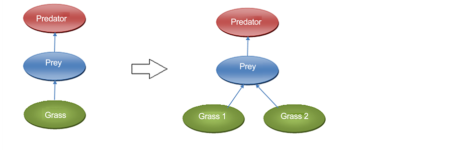
Figure A1. Regular food chain in EcoSim (a), and the new food chain in the modified dual resource EcoSim (b)
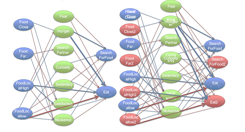
Figure A2. A part of the prey individuals’ FCM associated with grass consumption by prey in the single resource version of EcoSim (a) and in the dual resource version of EcoSim after introducing a new food resource and adding the new concepts (in red) (b). Note that the width of each edge shows the influence value of that edge and the color of an edge shows inhibitory (red) or excitatory (blue) effects.
Figure A3. The evaluation of the weighted sum of all incoming edges to Eat 1 and Eat 2 actions to determine species’ group.
Figure A4. Food resource preference distribution for Food1 (blue), Food2 (red), and Both foods (green). Each individual preference from the total prey population is calcu- lated for the duration of the simulation based on their FCM model.
Table A5. Five rules of Action-Perception Clustering.
*In order to be able to claim that the rate of one eating action is higher than the other, a threshold was applied for the minimum required differences between the rate of Eat 1 and Eat 2. This threshold has been defined so that the rate of one eating action should be twice as high as the other one to be counted as significantly greater. **Likewise, another threshold was used for the differences between available resources, to find out whether their abundances are approximately equal, or if one of them is more available than the other. Figure A5 presents the output of these species categorizing algorithms for one simulation, as an example of the resource preference distribution of all prey individuals based on their completed eating behaviors and their perception of available resources in their environment. The horizontal axis represents the time steps, while the vertical axis represents the percentage of prey belonging to each group. According to this figure, starting from around time step 21000, a significant proportion of the prey populations belong to both groups one and two. This provides an approximate time step to consider for indicators of sympatric speciation (exploring the four required criteria on those species).
Figure A5. Resource preference distribution based on the action-perception for Food 1 (blue), Food 2 (red), and Both resources (green). Each individual’s preference from the total prey population is calculated for the duration of the simulation based on their real eating behavior and their perception about the local food available.
Figure A6. The minimum distance, the average distance of the 200 closest individuals, and the average distance between all the individuals corresponding to two sister species at the speciation event and through subsequent time steps.
Table A6. List of initial attributes used to create the datasets, and a short description about each attribute.
Table A7. List of attributes and the result after applying attribute selection methods. The attributes highlighted in red were removed at the first step.
Figure A7. The decision tree returned by J48 classifier on all the datasets combined together, with 11 attributes and 20 rules.
Submit or recommend next manuscript to SCIRP and we will provide best service for you:
Accepting pre-submission inquiries through Email, Facebook, LinkedIn, Twitter, etc.
A wide selection of journals (inclusive of 9 subjects, more than 200 journals)
Providing 24-hour high-quality service
User-friendly online submission system
Fair and swift peer-review system
Efficient typesetting and proofreading procedure
Display of the result of downloads and visits, as well as the number of cited articles
Maximum dissemination of your research work
Submit your manuscript at: http://papersubmission.scirp.org/
Or contact oje@scirp.org
NOTES
1This work was made possible by the facilities of the Shared Hierarchical Academic Research Computing Network (SHARCNET): www.sharcnet.ca and Compute/Calcul Canada.


