Open Journal of Statistics
Vol.09 No.03(2019), Article ID:93485,34 pages
10.4236/ojs.2019.93026
Deep Language Statistics of Italian throughout Seven Centuries of Literature and Empirical Connections with Miller’s 7 ∓ 2 Law and Short-Term Memory
Emilio Matricciani
Dipartimento di Elettronica, Informazione e Bioingegneria (DEIB), Politecnico di Milano, Milan, Italy

Copyright © 2019 by author(s) and Scientific Research Publishing Inc.
This work is licensed under the Creative Commons Attribution International License (CC BY 4.0).
http://creativecommons.org/licenses/by/4.0/


Received: May 29, 2019; Accepted: June 27, 2019; Published: June 30, 2019
ABSTRACT
Statistics of languages are usually calculated by counting characters, words, sentences, word rankings. Some of these random variables are also the main “ingredients” of classical readability formulae. Revisiting the readability formula of Italian, known as GULPEASE, shows that of the two terms that determine the readability index G—the semantic index , proportional to the number of characters per word, and the syntactic index GF, proportional to the reciprocal of the number of words per sentence—GF is dominant because GC is, in practice, constant for any author throughout seven centuries of Italian Literature. Each author can modulate the length of sentences more freely than he can do with the length of words, and in different ways from author to author. For any author, any couple of text variables can be modelled by a linear relationship , but with different slope m from author to author, except for the relationship between characters and words, which is unique for all. The most important relationship found in the paper is that between the short-term memory capacity, described by Miller’s “7 ∓ 2 law” (i.e., the number of “chunks” that an average person can hold in the short-term memory ranges from 5 to 9), and the word interval, a new random variable defined as the average number of words between two successive punctuation marks. The word interval can be converted into a time interval through the average reading speed. The word interval spreads in the same range as Miller’s law, and the time interval is spread in the same range of short-term memory response times. The connection between the word interval (and time interval) and short-term memory appears, at least empirically, justified and natural, however, to be further investigated. Technical and scientific writings (papers, essays, etc.) ask more to their readers because words are on the average longer, the readability index G is lower, word and time intervals are longer. Future work done on ancient languages, such as the classical Greek and Latin Literatures (or modern languages Literatures), could bring us an insight into the short-term memory required to their well-educated ancient readers.
Keywords:
GULPEASE, Italian, Literature, Miller’s Law, Readability, Short-Term Memory, Word Interval

1. Introduction
Statistics of languages have been calculated for several western languages, mostly by counting characters, words, sentences, word rankings [1] . Some of these parameters are also the main “ingredients” of classical readability formulae. First developed in the United States [2] , readability formulae are applicable to any language, once the mathematical expression for that particular language is developed and assessed experimentally [3] . Readability formulae measure textual characteristics that are quantifiable, therefore mainly words and sentences lengths, by defining an ad hoc mathematical index. Therefore, according to the classical readability formulae, and solely on this ground, different texts can be compared automatically to assess the difficulty a reader should tolerate before giving up, if he is allowed to do so when he reads for pleasure not for duty, as is the case with technical and scientific texts [4] [5] [6] , which must be read because of technical or research activities, or for studying. In other words, readability indices allow matching texts to expected readers to the best possible, by avoiding over difficulty and inaccessible texts, or oversimplification, the latter felt as making fun of the reader.
Even after many years of studies and proposals of many readability formulae, especially for English [3] [7] [8] [9] , nobody, as far as I know, has shown a possible direct relationship of a readability formula and its constituents (characters, sentences etc.), with reader’s short-term memory behavior [10] [11] [12] [13] . In this paper, I show that a statistical relationship can be found for Italian, by examining a large number of literary texts written since the XIV century, thus revitalizing the classical readability formula approach.
The classical readability formulae, in fact, have been criticized because they focus on a limited set of superficial text features, rough approximations of the linguistic factors at play in readability assessment [14] . However, a readability formula does measure important constituents of texts and can contribute to understanding the process of communication, especially if its ingredients relate to the storage of information in the short-term memory. Moreover, because an “absolute” (i.e. a formula that provides numerical indices counted from a universal origin, such as zero) readability formula might not exist at all, the current formulae can be used to compare different texts, together with other parameters which I define in this paper. In other words, differences between the numerical values given by a readability formula—i.e. relative indices—may be more significant than absolute ones for the purpose of comparing texts, especially literary texts, as done in this paper. In spite of this, in the following I will present absolute values because readers are used to considering them when they apply readability formulae, but I also discuss differences, which the reader can appreciate from the numerical values reported in the tables or in the scatter plots below.
In spite of the long-lasting controversy on the development and use of classical readability formulae, researchers still continue to develop methods to overcome weaknesses by advancing natural language processing and other computerized language methods [15] [16] , to capture more complex linguistic features [17] . Benjamin [15] , however, predicts that also in this research field will happen what does happen in any research field when no general consensus is shared on a specific topic, that is, that also these new developments will be judged controversial. In any case, the classical readability formulae have served their purpose in leveling typical books for schoolchildren and general audience, such as in Italy in the 1980s [18] .
Now, new methods, developed after cognitive processing theories, should allow analyzing more complex texts for specific targets such as adolescents, university students, and adults. Moreover, with machine-learning developments, non-traditional texts, like those found in many web sites, can be categorized for greater accessibility. Some of these advances concern even observing eye tracking while reading [16] [19] . For Italian, the work by Dell’Orletta and colleagues [17] aims at automatically assessing the readability of newspaper texts with the specific task of text simplification, not for specifically analyzing and studying literary texts and their statistics, as I do in this paper.
A readability formula is, however, very attractive because it allows giving a quantitative and automatic judgement on the difficulty or easiness of reading a text. Every readability formula, however, gives a partial measurement of reading difficulty because its result is mainly linked to words and sentences length. It gives no clues as to the correct use of words, to the variety and richness of the literary expression, to its beauty or efficacy, does not measure the quality and clearness of ideas or give information on the correct use of grammar, does not help in better structuring the outline of a text, for example a scientific paper. The comprehension of a text (not to be confused with its readability, defined by the mathematical formulae) is the result of many other factors, the most important being reader’s culture and reading habits. In spite of these limits, readability formulae are very useful, if we apply them for specific purposes, and assess their possible connections with the short-term memory of readers.
Compared to the more sophisticated methods mentioned above the classical readability formulae have several advantages:
1) They give an index that any writer (or reader) can calculate directly, easily, by means of the same tool used for writing (e.g. WinWord), therefore sufficiently matching the text to the expected audience.
2) Their “ingredients” are understandable by anyone, because they are interwound with a long-lasting writing and reading experience based on characters, words and sentences.
3) Characters, words, sentences and punctuation marks appear to be related to the capacity and time response of short-term memory, as shown in this paper.
4) They give an index based on the same variables, regardless of the text considered, thus they give an objective measurement for comparing different texts or authors, without resorting to readers’ physical actions or psychological behavior, which largely vary from one reader to another, and within a reader in different occasions, and may require ad hoc assessment methods.
5) A final objective readability formula or more recent software-developed methods valid universally are very unlikely to be found or accepted by everyone. Instead of absolute readability, readability differences can be more useful and meaningful. The classical readability formulae provide these differences easily and directly.
In this paper, for Italian, I show that a relationship between some texts statistics and reader’s short-term memory capacity and response time seems to exist. I have found an empirical relationship between the readability formula mostly used for Italian and short-term memory capacity, by considering a very large sample of literary works of the Italian Literature spanning seven centuries, most of them still read and studied in Italian high schools or researched in universities. The contemporaneous reader of any of these works is supposed to be, of course, educated and able to read long texts with good attention. In other words, this audience is quite different of that considered in the studies and experiments reported above on new techniques (based on complex software) for assessing readability of specific types of texts [17] . In other words, the subject of my study are the ingredients of a classical readability formula, not the formula itself (even though I have found some interesting features and limits of it), and its empirical relationship with short-term memory. From my results, it might be possible to establish interesting links to other cognitive issues, as discussed by [20] , a task beyond the scope of this paper and author’s expertise.
The most important relationship I have found is that between the short-term memory capacity, described by Miller’s “7 ∓ 2 law” [21] , and what I call the word interval, a new random variable defined as the average number of words between two successive punctuation marks. The word interval can be converted into a time interval through the average reading speed. The word interval is numerically spread in a range very alike to that found in Miller’s law, and more recently by Jones and Macken [12] , and the time interval is spread in a range very alike to that found in the studies on short-term memory response time [10] [22] [23] . The connection between the word interval (and time interval) and short-term memory appears, at least empirically, justified and natural, but at this stage is a well-educated guess.
Finally, notice that in the case of ancient languages, no longer spoken by a people but rich in literary texts, such as Greek or Latin, that have founded the Western civilization, it is obvious that nobody can make reliable experiments, as those reported in the references recalled above. These ancient languages, however, have left us a huge library of literary and (few) scientific texts. Besides the traditional count of characters, words and sentences, the study of word and time intervals statistics should bring us an insight into the short-term memory features of these ancient readers, and this can be done very easily, as I have done for Italian. An analysis of the New Testament Greek originals [24] , similar to that reported in this paper, shows results very similar to those reported in this paper, therefore evidencing some universal and long-lasting characteristics of western languages and their readers.
In conclusion, the aim of this paper is to research, with regard to the high Italian language, the following topics:
1) The impact of character and sentence indices on the readability index (all defined in Section 2).
2) The relationship of these indices with the newly defined “word interval” and “time interval”.
3) The “distance”, absolute and relative, of literary texts by defining meaningful vectors based on characters, words, sentences, punctuation marks.
4) The relationship between the word interval and Miller’s law, and between the time interval and short-term memory response time.
After this Introduction, Section 2 revisits the classical readability formula of Italian; Section 3 shows interesting relationships between its constituents; Section 4 reports the statistical results for a large number of texts of the Italian Literature since the XIV century; Section 5 discusses the “distance” of literary texts; Section 6 introduces word and time intervals and their empirical relationships with short-term memory features; Section 7 discusses some different results concerning scientific and technical texts, and finally Section 8 draws some conclusions and suggests future work.
2. Revisiting the GULPEASE Readability Formula of Italian
For Italian, the most used formula (calculated by WinWord, for example), known with the acronym GULPEASE [25] , is given by:
(1a)
The numerical values of Equation (1a) can be interpreted as readability index for Italian as a function of the number of years of school attended in Italy’s school system [25] , as I have graphically summarized in Figure 1. The larger G, the more readable the text is. In Equation (1a) p is the total number of words in the text considered, c is the number of letters contained in the p words, f is the
Figure 1. Readability index G of Italian, as a function of the number of school years attended (in Italy high school lasts 5 years, children attend it up to 19 years old). The blue thinner lines indicate the error bounds found in using Equation (6). Elementary school lasts 5 years, Scuola Media Inferiore lasts 3 years, Scuola Media Superiore (High School) lasts 5 years (the vertical magenta line shows the beginning of High School).
number of sentences contained in the p words (a list of mathematical symbols is reported in the Appendix). Let us define the terms:
(2a)
(2b)
Therefore, Equation (1a) can be written as:
(1b)
We analyze first Equations (1a) (1b), by means of standard statistics of its addends, because, as other readability formulae, they contain important characteristics of literary texts which for the Italian Literature, that extends for the longest period of time compared to other modern western languages, have been stable over centuries (namely GC).
Equation (1) says that a text, for the same amount of words, is more difficult to read if is small, hence if sentences are long, and if the number of characters per word is large, hence if words are long. Long sentences
mean that the reciprocal value is large, therefore there are many
words in a sentence, GF decreases and thus G decreases. The sentences contain many subordinate clauses, the reading difficulty is due to syntax and therefore we term loosely the syntactic index. Long words mean that GC increases, it is subtracted from the constant 89 and thus G decreases. Long words often refer to abstract concepts (maybe of Latin or Greek origin), difficulty is due to characters, and therefore we term loosely GC the semantic index. In other words, a text is easier to read if it contains short words and short sentences, a known result applicable to readability formulae of any language.
Now, the study of Equation (1), and in particular how the two terms , GF affect the value of G, brings very interesting results, as we show next. In this paper I apply the above equations to classical literary works of a large number of Italian writers1, from Giovanni Boccaccio (XIV century) to Italo Calvino (XX century), see Table 1, by examining some complete works, as they are available today in their best edition2.

Table 1. Characters, words and sentences in the literary works considered in this study, and average values of the corresponding G, GC e GF, the standard deviation of averages ( in parentheses) and the standard deviation estimated for text blocks of 1000 words3. The characters are those contained in the words. All parameters have been computed by weighting the text blocks according to the number of the words contained in them. For instance, in Decameron, the average value of G can be estimated in 51.18 ± 0.17 and its standard deviation for text blocks of 1000 words is 2.85.
3. Relationships among GC, GF and G
The semantic index , given by the number of characters per word multiplied by 10 (Equation (2a)), and the syntactic index GF, given by the reciprocal of the number of words per sentence PF, multiplied by 300 (Equation (2b)), affect very differently the final value of G (Equation (1b)). Table 1 lists the average values of G, GC, GF and their standard deviations for the literary works considered. In this analysis, as in the successive ones, I have considered text blocks, singled out by an explicit subdivision of the author or editor (e.g., chapters, subdivision of chapters, etc.), without titles. This arbitrary selection does not affect average values and the standard deviations of these averages. All parameters have been calculated by weighting any text block with its number of words, so that longer blocks weigh statistically more than shorter ones as detailed in the following.
Let
average value is given by
with
,
the number of words and sentences contained in the text block i-th. For the standard deviation of the average value, we calculate first the average square value
and the standard deviation in the
From the results reported in Table 1, it is evident that GC changes much less than GF, a feature highlighted in the scatter plot of Figure 2(a), which shows GC and GF versus G, for each text block (1260 text blocks in total, with different number of words) found in the listed literary works.
The theoretical range of G can be calculated by considering the theoretical range of GF. The maximum value of GF is found when PF is minimum, the latter given by 1 when , therefore when all sentences are made of 1 single word, hence , a case obviously not realistic. A more realistic maximum value can be estimated by considering 4 or 5 words per sentence, so that reduces to 75 or 60. The minimum value is obviously , i.e., the text is made of 1 sentence with an infinite (very large) number of words. In conclusion, by considering the average value of (Table 1), the GULPEASE index can theoretically range from to (close to the smallest values in Table 1).
The constancy of GC versus G indicates that, in Italian, the number of characters per word CP has been very stable over many centuries, while the linear proportionality between GF and G, is directly linked to author’s style, or to the style applied to different works by the same author. With “style” I refer to the writer’s choice of sentence length and punctuation marks distribution within the sentence, namely to the variables of interest in my mathematical approach. These features are confirmed in Figure 2(b), which shows the scatter plots of the average number of characters per word CP vs. G, and PF vs. G In other words, the
 (a)
(a) (b)
(b)
Figure 2. (a) GC (blue circles) and GF (cyan crosses) versus G, for all 1260 text blocks. BC = Boccaccio, MN PS = Manzoni (I promessi sposi), CL = Collodi, CS = Cassola. The horizontal line is the average value of GC, Equation (3), the diagonal line is the average value of GF, Equation (4); (b) Scatter plots of vs. G (blue dots) and vs. G (cyan crosses). BC = Boccaccio, MN PS = Manzoni (I promessi sposi), CL = Collodi, CS = Cassola. The black continuous lines are given by Equations (3) and (5).
readability of a text using (1) is practically due only to the syntactic index GF, therefore to the number of words per sentence. The two lines drawn in Figure 2(a) are given by the average value of GC (Table 2):
Table 2. Average values of a number of characters per word, words per sentence, punctuation marks per sentence and punctuation interval. Standard deviations calculated as in Table 1.
(3)
and the average value of GF described by the regression line
(4)
The correlation coefficient between GF and G, Equation (4), is 0.932. The slope is 0.912, therefore, giving practically a 45˚ line. By considering the coefficient of variation, of the data is explained by (4). Figure 2(a) shows also the average values of selected works listed in Table 1 to locate them in this scatter plot. Figure 2(b) shows, superposed to the scattered values of PF, the theoretical relationship between the average value of PF, as a function of G, given, according to Equations (1a) and (3), by:
(5)
The correlation between the experimental values of PF and that calculated from (5) is 0.800. The correlation between the experimental values of PF and G is −0.830.
In conclusions, Equation (1a) can be rewritten by modifying the constant from 89 to 42.3, without significantly changing the numerical values of Equation (1), but now giving a meaning to the constant 42.3, as the minimum value , so that (1) can be written as:
(6)
From these results, it is evident that each author has his own “dynamics”, in the sense that each author modulates the length of sentences in a way significantly more ample than he does or, I should say, he could do with the length of words, and differently from other authors, as we can read in Table 2. We pass, for example, from 11.93 words per sentence (Cassola) to 44.27 words per sentence (Boccaccio), whereas the number of characters per word ranges only from 4.481 to 4.475, a much smaller range. Even if the two authors are spaced centuries apart, have very different literary style, write very different novels and address very different audiences—all characteristics well-known in the history of Italian Literature—both use words of very similar length.
The average number of characters per word, CP, varies between 4.37 (Bembo, Sacchetti) and 5.01 (Salgari), a range equal to 0.64 characters per word which, compared to the global average value 4.67 (Table 2), corresponds to ∓ 6.8% change. On the contrary, GF varies from 6.94 (Boccaccio) to 25.65 (Cassola), with excursions in the range from −52% to ∓78%, compared to the global average value 14.40 (Table 1). Of course, the values of each text block can vary around the average, as for example Figure 3 and Figure 4 show for Boccaccio and Manzoni, because of different types of literary texts, such dialogues, descriptions, author’s considerations or comments, etc. On the other hand, the reader that wishes to read it all is exposed to the full variety of texts, which in any case must be read. In other words, what counts is the average value of a parameter, not the variations that it can assume in each text block, as also Martin and Gottron underline [26] .
By considering the above findings, we can state that GC is practically a constant, , and that G can be approximated by (6).
Figure 3. Ordered text-block series of G, , GF, PF, MF and Ip, versus the ordered sequence of text blocks found in Boccaccio’s Decameron. The text blocks are the novels told, on turn, by each character each day. The horizontal magenta lines give the average values (Table 1 and Table 2).
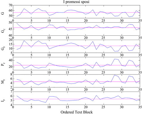
Figure 4. Ordered text-block series of G, , GF, PF, MF and Ip, versus the ordered sequence of text blocks found in Manzoni’s I promessi sposi. The text blocks are the chapters. The horizontal magenta lines give the average values (Table 1 and Table 2).
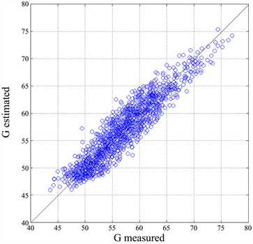
Figure 5(a) shows the scatter plot between the values calculated with Equation (6) by using the value of GF of each text block, and the values calculated with Equation (1a), and the regression line between the two data sets. The slope is 0.998, in practice 1 (45˚ line), and the correlation coefficient is4 0.932.
Defined the error , its average value is −0.1, therefore 0 for any practical purpose, and its standard deviation is 2.14. For a constant readability level G, the latter value translates into an estimating error of school years required by at most 1 year, see Figure 1. Figure 5(b) shows that a normal (Gaussian) probability density function with zero average value and standard deviation 2.14 describes very well the error scattering.
 (a)
(a)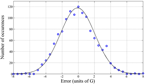 (b)
(b)
Figure 5. (a) Scatter plot of Equation (6), and the values G calculated with Equation (1). Also shown the regression line, in practice the 45˚line ; (b) Histogram of the error (blue circles) and theoretical histogram (black line) due to a Gaussian (normal) density function with average value −0.1 and standard deviation 2.14.
Now, according to (6) it is obvious that the constant value can be set to zero, therefore making:
(7)
with the advantage that the scaled index Gs starts at 0. Now Equation (7) is not meant to be used to reduce any computability effort, as today Equation (1), like any other readability formula or other approaches, can be calculated by means of dedicated software, with no particular effort. Equation (7) is useful because underlines the fact that authors of the Italian Literature modulate much more the length of sentences, and each of them with personal style, than the length of words, and that the length of sentences substantially determines reading difficulty (as any Italian student knows when reading Boccaccio’s Decameron, or Collodi’s Pinocchio!), so that we could use Figure 6, as a guide, instead of Figure 1.
4. Characters, Words, Sentences, Punctuation Marks, Word and Time Intervals
Table 3 shows that, for any author, there is a large correlation, close to unity, between the number of characters and the number of words, as Figure 7 directly shows. The correlation coefficient is 0.999 and the slope of the line is characters per word, equal to the average value (Table 2), because the correlation coefficient is very close to 1. On the average, every word in the Italian literature is made of 4.67 ∓ 0.006 characters, so that characters and words can be interchanged in any mathematical relationship.
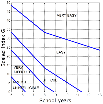
Figure 6. Scaled index GS as a function of the number of school years attended in the Italian School System.
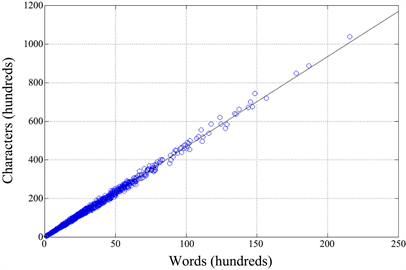
Figure 7. Scatter plot between the number of characters and the number of words (1260 text blocks), also shown the regression line (see Table 3).
Table 3. Correlation coefficient and slope (in parentheses) of the line modelling the indicated variables.
The relationship between words and sentences behaves differently. For each author a line still describes, usually very well, their relationship (see Table 2 and Table 3), but with different slope, as Figure 8 shows. The average number of words per sentence varies from 11.93 (Cassola) to 44.47 (Boccaccio) and these values affect very much the sentence term GF, which varies from 25.65 (Cassola) to 6.94 (Boccaccio). In Figure 8, we can notice that there is an angular range where all authors fall, a range that has collapsed into a line in Figure 7 because of a very tight, and equal for all authors, relationship between characters and words. Moreover, notice that the value of calculated from the average GF, i.e. , is always smaller or at most equal5 to the average value of the ratio (Table 2).
Defined the total number of punctuation marks (sum of commas, semicolons, colons, question marks, exclamation marks, ellipsis, periods) contained in a text, Figure 9 shows the scatter plot between this value and the number of sentences for each text block. Once more, for any author the relationship is a line with correlation coefficients close to 1 (Table 3), but with different slopes, the latter close to the average number of punctuation marks per sentence. For example, in Boccaccio, the average number of punctuation marks per sentence is (Table 2), whereas the slope6 of the corresponding line is (Table 3).
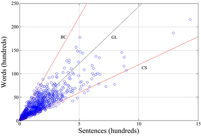
Figure 8. Scatter plot between the number of words and the number of sentences (1260 text blocks). BC refers to Boccaccio, CS refers to Cassola, GL refers to the global values. The two authors represent approximate bounds to the angular region.
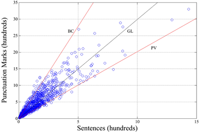
Figure 9. Scatter plot between the number of punctuation marks and the number of sentences (1260 text blocks). BC refers to Boccaccio, PV refers to Pavese (La bella estate), GL refers to the global values. The two authors represent approximate bounds to the angular region. The ratio between the ordinate and the abscissa gives the word interval.
An interesting comparison among different authors and their literary works can be done by considering the number of words per punctuation mark, that is to say, the average number of words between two successive punctuation marks, a random variable that is the word interval Ip mentioned before, defined by:
(8)
The word interval IP is very robust against changing habits in the use of punctuation marks throughout decades. Punctuation marks are used for two goals: 1) improving readability by making lexical and sentence constituents of texts more easily recognizable, 2) introducing pause [27] , and the two goals can coincide [28] [29] . In the last decades, in Italian, there has been a reduced use of semicolons in favor of periods [30] , but this change does not affect IP but only the number of words per sentence.
The values of IP listed in Table 2 vary from 5.64 (Cassola) to 7.8 (Boccaccio). For any author, the linear model is still valid, as the high correlation coefficients listed in Table 3 and Figure 10 show. The slopes of the lines are very close to the averages, namely 5.56 and 7.82 respectively, because of correlation coefficients7 close to 1.
Finally, Figure 11 shows the scatter plot between G, GC, GF and Ip. We can notice that GF (and G) is significantly correlated with IP through an inverse proportionality. This result is very interesting because it links the readability of a text, the index G, or GF, to Ip, another author’s distinctive characteristic. Moreover, the word interval has other very interesting and intriguing relationships, as section 5 shows.
5. Comparing Different Literary Texts: Distances
A large number of texts produced today in several forms, both in hard copies and digital formats, such as books, journals, technical reports and others, have prompted several methods for fast automatic information retrieval, document classification, including authorship attribution. The approach is to represent documents with n-grams using vector representation of particular text features [31] . In this model, the similarity between two documents is estimated using the cosine of the angle between the corresponding vectors. This approach depends mainly on the similarity of the vocabulary used in the texts, while the characters and syntax are ignored. A more complex approach represents textual data in more detail [31] . These new techniques, implemented with complex software, are useful when, together with other tasks, automatic authorship attribution and verification are required.
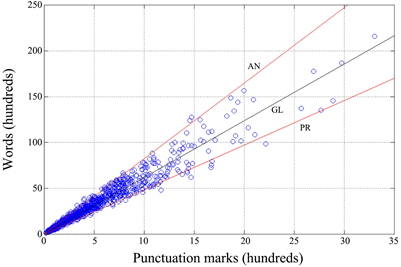
Figure 10. Scatter plot between the number of words and the number of punctuation marks (1260 text blocks). AN refers to Anonymous, PR refers to Pirandello, GL refers to the global values. The two authors represent approximate bounds to the angular region. The ratio between the ordinate and the abscissa gives the word interval.
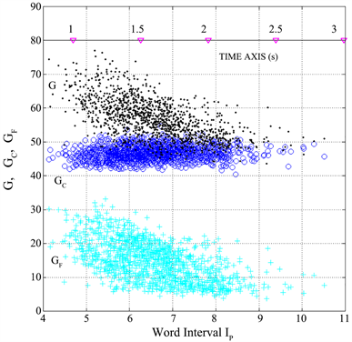
Figure 11. Scatter plot between G (black dots), GC (blue circles), GF (cyan crosses) and the word interval Ip. The top time axis refers to the time interval IT (Section 6).
In the case of the literary texts considered in this paper, it is more interesting to compare the statistical characteristics of different authors or different texts of the same author, by using the data reported in Tables 1-3, instead of using the more complex methods reviewed by [32] . For this purpose, the parameters that are most significant are the four random variables defined before: CP, PF, MF and IP, because they represent fundamental indices and are mostly uncorrelated, except the couple (MF, IP), as Table 4 shows. These parameters are suitable to assess similarities and differences of texts much better, as I show next, than the cosine of the angle between any two vectors. Therefore, in this section, I define absolute and relative “distances” of texts by considering the following six vectors of components8 x and y: , , , , , .
Now, considering the six vectors just defined, the average cosine similarity S between two documents (literary texts) D1 and D2 can be computed as:
(9)
where is the cosine of the angle formed by the two vectors . If all pairs of vectors were collinear (aligned), then , the similarity would be maximum, . If all pairs of vectors were orthogonal , the similarity would be zero, . According to this criterion, two collinear vectors of very different length (the magnitude of the vector) will be classified as identical because , a conclusion that cannot be accepted. This is a serious drawback of the cosine similarity.
Figure 12 shows the scatter plot between the average value of S, calculated by considering all text blocks, and the readability index G. Any text block is compared also to another text block of the same literary text (but not with itself). The choice of not excluding the other text blocks of the same literary text leads to a simple and straight software code, which, however, does not affect the general conclusion arrived at by observing the scatter plot shown in Figure 12: there is no correlation between S and G, therefore S does not meaningfully discriminate between any two texts when the angle formed by their vectors is close to zero.
Table 4. Linear correlation coefficients between the indicated pairs of random variables (1260 text blocks).
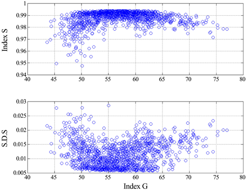
Figure 12. Upper panel: Scatter plot between the average similarity index S of a text block, out of 1260 in total, about all others, and the corresponding readability index G. Lower panel: standard deviation. The total amount of data used to calculate average and standard deviation is given by .
Now, a better choice for comparing literary texts is to consider the “distance” of any text block from the origin of x and y axes9, given by the magnitude of the resulting vector :
(10)
With this vectorial representation, a text block ends up in a point of coordinates x and y in the first Cartesian quadrant, as Figure 13 shows. The end point of the vectors with components given by the average values of the literary texts (obtainable from Tables 1-3) is also shown.
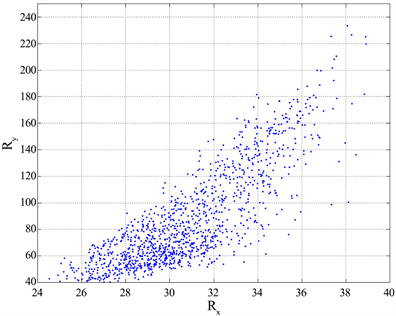
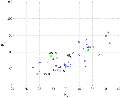
Figure 13. Scatter plot between the two components of the distance R for all 1260 text block (upper panel), and that calculated from the average values shown in Tables 1-3 (lower panel). CS = Cassola, PV B = Pavese La bella estate, PV F = Pavese La luna e i falò, MN PS = Manzoni I promessi sposi, MN FL = Manzoni Fermo e Lucia, FG = Fogazzaro Il santo and Piccolo mondo antico, BC = Boccaccio, GL = global values (“barycentre”).
It is very interesting, for example, to compare the vector representing Manzoni’s masterpiece10 I promessi sposi (published in 1840) and that representing Manzoni’s Fermo e Lucia (published in 1827). The latter novel was the first version of I promessi sposi and the great improvement pursued by Manzoni in many years of revision, well known to scholars of Italian literature, is also observable mathematically: the absolute distances are 113.9 for Fermo e Lucia and 93.7 for I promessi sposi, the relative distance is 20.3, a significant fraction of the entire range spanning from Cassola to Boccaccio, whose relative distance is 106.611. Other interesting observations are the coincidence of the two vectors representing the novels by Fogazzaro, and the difference between the novels by Pavese, etc. With this tool, the scholars of Italian literature (even if not accustomed to using mathematics in their research) could find some objective confirmation of their literary studies concerning an author, as exemplified in the case of Manzoni.
The efficacy of can be appreciated in Figure 14, which shows the scatter plot between R and G, and between its angle , expressed in degrees, and G. The black lines describe very well the relationships between them, given by:
(11a)
(11b)
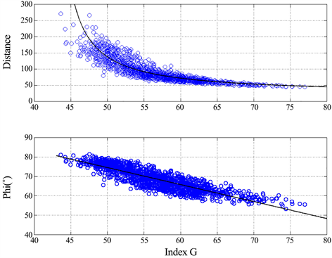
Figure 14. Scatter plot between R and G (upper panel) and between and G (lower panel).
The correlation coefficient is −0.832, for the couple and −0.867 for the couple . The correlation coefficient between measured and estimated values of R through (11a) is 0.802 between the measured and estimated values of with (11b) is12 0.867. In conclusion, the magnitude (distance) R and the angle of the vector are very well correlated with the readability index G.
6. Word Interval, Miller’s 7 ∓ 2 Law and Short-Term Memory Capacity
The range of the word interval Ip, shown in Figure 11, is very similar to the range mentioned in Miller’s law 7 ∓ 2, although the short-term memory capacity of data for which chunking is restricted is 4 ± 1 [33] [34] [35] [36] [37] . For words, namely data that can be restricted (i.e., “compressed”) by chunking, it seems that the average value is not 7 but around 5 to 6 [21] , almost the average value of the word interval 6.56 (Table 2). Now, as the range from 5 to 9 in Miller’s law corresponds to 95% of the occurrences [37] , it is correct to compare Miller’s interval with the dispersion of the word interval in single text block shown in Figure 11, where we can see values ranging from 4 to 10.5, close to Miller’s law range.
The probability density function and the complementary probability distribution of IP are shown in Figure 15. From the lower panel we can see that 95% of the samples (probabilities between 0.025 and 0.975) fall in the range from 4.6 to 8.6, which concides, in practice, with Miller’s range 7 ± 2. The most likely value (the mode of the distribution) is 6.3 and the median is 6.5. The experimental density can be modelled with a log-normal model with three parameters:
(12a)
with confidence level in excess of 99.99% (chi-square test) [38] . The log-normal probability density is valid only for being the minimum theoretical value of this variable (a single sentence made of only 1 word).
The theoretical constants of Equation (12) are obtained as follows. Given the average value and the standard deviation , of the random variable IP for the 1260 text blocks, the standard deviation and the average value of the random variable of a three-parameter log-normal probability density function [39] are given (natural logs) by:
(12b)
(12c)
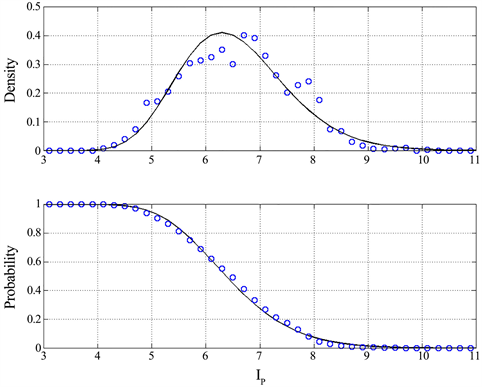
Figure 15. Probability density function (upper panel, blue circles) and the complementary probability distribution (lower panel, blue circles) of IP for 1260 text blocks. The lower panel shows the probability that the value reported in abscissa (x axis) is exceeded. The black continuous lines are the theoretical density and distribution of a three-parameter log-normal model [39] .
The theoretical mode (the most likely value) is given by . Notice, however, that the experimental mode observed in Figure 15 is near 7, very close to the central value of Miller’s range and that an underlying mixture of three shifted probability distributions may be a better model. However, for the purpose of linking the word interval IP to the short-term memory capacity this analysis may be sufficient.
These results may be explained, at least empirically, according to the way our mind is thought to memorize “chunks” of information in the short-term memory. When we start reading a sentence, our mind tries to predict its full meaning from what has been read up to that point, as it seems that can be concluded from the experiments of Jarvella [40] . Only when a punctuation mark is found, our mind can better understand the meaning of the text. The longer and more twisted is the sentence, the longer the ideas remain deferred until the mind can establish the meaning of the sentence from all its words. In this case, the text is less readable, a result quantitatively expressed by the empirical Equation (1a) for Italian.
Figure 16 shows the scatter plot between Ip and PF for all the text blocks, together with the non-linear regression line (best-fit line) that models, on the average, Ip versus PF for the Italian Literature, given by:
(13)
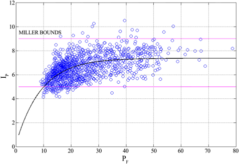
Figure 16. Scatter plot between the word interval IP and the number of words per sentence PF for all text blocks. The continuous black line refers to the best fit given by Equation (13). Also shown the 7 ∓ 2 bounds of Miller’s Law (magenta lines).
where words per interpunctions is the horizontal asymptote, and words per sentence is the value of PF at which the exponential in Equation (13) falls at 1/e of its maximum value. Notice that: 1) most data fall in the Miller’s range 7 ∓ 2; 2) the asymptotic value (7.37) is very close to the center value of Miller’s range; 3) is the abscissa corresponding to the lower bound of Miller’s law.
These results can be explained as follows. As the number of words increases, the number of word intervals can increase but not linearly, because the short-term memory cannot hold, approximately, a number of words larger than that empirically described by Miller’s Law. In other words, scatter plots like that shown in Figure 16 drawn for other Literatures—classical Greek and Latin Literatures, or modern languages Literatures—should give us an insight into the short-term memory capacity required to their readers.
In conclusion, the range of the word interval is similar to Miller’s law range. The values found for each author seems to set the size of the short-term memory capacity that their readers should have to read the literary work more easily. For example, the reader of Boccaccio’s Decameron should have a short-term memory able to memorize chunks, on the average, whereas the reader of Collodi’s Pinocchio needs only a memory of capacity chunks. Now, if our conjecture is found reliable after more studies concerning short-term memory and brain, the link between GF and G through Equation (6), would appear justified and natural.
The word interval can be translated into a time interval if we consider the average reading speed of Italian, estimated in 188 words per minute [41] . In this case, the average time interval corresponding to the word interval, expressed in seconds, is given by:
(14)
The time axis drawn in Figure 11 is useful to convert IP into IT. The values of IP shown in the scatter plot, now read as time interval, according to the time scale agree very well with the intervals of time so that the immediate memory records the stimulus for later memorizing it in the short term memory, ranging from 1 to about 2-3 seconds [10] [13] [22] [23] [42] [43] .
The results, relating IT and IP to fundamental and accessible characteristics of short-term memory, are very interesting and should be furtherly pursued by experts. Moreover, the same studies can be done on ancient languages, such as Greek and Latin, to test the expected capacity and response time of the short-term memory of these ancient and well-educated readers, partially already done for the Greek of the New Testament [24] .
7. Technical and Scientific Writings
Technical and scientific writings (papers, essays, etc.) ask more to their readers. A preliminary investigation was done on short scientific texts published in the Italian popular science magazines Le Scienze and Sapere (because today is rare to find original scientific papers written in Italian), in a popular scientific book and newspaper editorials gave the results listed in Table 5. In this analysis, mathematical expressions, tables, legends have not been considered. From Table 5 we can notice some clear differences from the results of novels: words are on the average longer, the readability index G is lower, the word interval is longer. These results are not surprising because technical and scientific writings use long technical words, deal with abstract meaning with articulated and elaborated sentences resulting in long sentences with series of subordinate clauses. Of course, the reader of these texts expects to find technical and abstract terms of his field, or specialty, and would not understand the text if these elements were absent.
8. Conclusions and Future Developments
Statistics of languages have been calculated for several western languages, mostly by counting characters, words, sentences, word rankings. Some of these parameters are also the main “ingredients” of classical readability formulae. Revisiting the readability formula of Italian, known with the acronym GULPEASE, shows that of the two terms that determine the readability index G—the semantic index GC, proportional to the number of characters per word, and the syntactic index GF, proportional to the reciprocal of the number of words per sentence—GF is dominant because GC is, in practice, constant for any author. From these results, it is evident that each author modulates the length of sentences more freely than what he can do with word length and in different ways from author to author.
Table 5. Statistics of some recent texts extracted from popular scientific literature and daily newspapers comments and short essays.
For any author, any couple of text variables can be described by a linear relationship but with different slope m from author to author, except for the relationship between characters and words, which is unique.
The most important relationship I have found is that between the short-term memory capacity, described by Miller’s “7 ∓ 2 law”, and what I have termed the word interval, a new random variable defined as the average number of words between two successive punctuation marks. The word interval can be converted into a time interval through the average reading speed. The word interval is numerically spread in a range very alike to that found in Miller’s law, and the time interval is spread in a range very alike to that found in the studies on short-term memory response time. The connection between the word interval (and time interval) and short-term memory appears, at least empirically, justified and natural.
For ancient languages, no longer spoken by a people, but rich in literary texts that have founded the Western civilization, such as Greek or Latin, nobody can make reliable experiments, as those reported in the references recalled above. These ancient languages, however, have left us a huge library of literary and (few) scientific texts. Besides the traditional count of characters, words and sentences, the study of their word interval statistics should bring us a flavor of the short-term memory features of these ancient readers, and this can be done very easily, as I have done for Italian. A preliminary analysis of a large number of Greek and Latin literary texts shows results very similar to those reported in this paper, therefore evidencing some universal and long-lasting characteristics of western languages and their readers.
In conclusion, it seems that there is a possible direct and interesting connection between readability formulae and reader’s capacity of short-term memory capacity and response time. As short-term memory features can be related to other cognitive parameters [20] , this relationship seems to be very useful. However, its relationship with Miller’s law should be further investigated because the word interval is another parameter that can be used to design a text, together with readability formulae, for better matching expected reader’s characteristics.
Acknowledgments
I am very grateful to Liber Liber (https://www.liberliber.it/online/opere/libri/) for providing the digital versions of the classics of Italian Literature. Without this large texts bank, I could not have ever obtained the results reported in the paper.
Conflicts of Interest
The authors declare no conflicts of interest regarding the publication of this paper.
Cite this paper
Matricciani, E. (2019) Deep Language Statistics of Italian throughout Seven Centuries of Literature and Empirical Connections with Miller’s 7 ∓ 2 Law and Short-Term Memory. Open Journal of Statistics, 9, 373-406. https://doi.org/10.4236/ojs.2019.93026
References
- 1. Grzybeck, P. (2007) History and Methodology of Word Length Studies. In: Contributions to the Science of Text and Language, Springer, Dordrecht, 15-90. https://doi.org/10.1007/1-4020-4068-7_2
- 2. DuBay, W.H. (2004) The Principles of Readability. Impact Information, Costa Mesa.
- 3. DuBay, W.H. (2006) The Classic Readability Studies. Impact Information, Costa Mesa.
- 4. Anderson, P.V. (1991) Technical Writing: A Reader-Centered Approach. 2nd Edition, Harcourt Brace Jovanovich, Fort Worth.
- 5. Burnett, R.E. (2004) Technical Communication. 3rd Edition, Wadsworth Publishing Company, Belmont.
- 6. Matricciani, E. (2007) La scrittura tecnico-scientifica. Casa Editrice Ambrosiana, Milano.
- 7. Saaty, T.L. and Ozdemir, M.S. (2003) Why the Magic Number Seven Plus or Minus Two. Mathematical and Computer Modelling, 38, 233-244. https://doi.org/10.1016/S0895-7177(03)90083-5
- 8. Zamanian, M. and Heydari, P. (2012) Readability of Texts: State of the Art. Theory and Practice in Language Studies, 2, 43-53. https://doi.org/10.4304/tpls.2.1.43-53
- 9. Collins-Thompson, K. (2014) Computational Assessment of Text Readability: A Survey of Past, in Present and Future Research, Recent Advances in Automatic Readability Assessment and Text Simplification, ITL. International Journal of Applied Linguistics, 165, 97-135. https://doi.org/10.1075/itl.165.2.01col
- 10. Baddeley, A.D., Thomson, N. and Buchanan, M. (1975) Word Length and the Structure of Short-Term Memory. Journal of Verbal Learning and Verbal Behavior, 14, 575-589. https://doi.org/10.1016/S0022-5371(75)80045-4
- 11. Barrouillest, P. and Camos, V. (2012) As Time Goes By: Temporal Constraints in Working Memory. Current Directions in Psychological Science, 21, 413-419. https://doi.org/10.1177/0963721412459513
- 12. Jones, G. and Macken, B. (2015) Questioning Short-Term Memory and Its Measurements: Why Digit Span Measures Long-Term Associative Learning. Cognition, 144, 1-13. https://doi.org/10.1016/j.cognition.2015.07.009
- 13. Chekaf, M., Cowan, N. and Mathy, F. (2016) Chunk Formation in Immediate Memory and How It Relates to Data Compression. Cognition, 155, 96-107. https://doi.org/10.1016/j.cognition.2016.05.024
- 14. Bailin, A. and Graftstein, A. (2001) The Linguistic Assumptions Underlying Readability Formulae: A Critique. Language & Communication, 21, 285-301. https://doi.org/10.1016/S0271-5309(01)00005-2
- 15. Benjamin, R.G. (2012) Reconstructing Readability: Recent Developments and Recommendations in the Analysis of Text Difficulty. Educational Psychology Review, 24, 63-88. https://doi.org/10.1007/s10648-011-9181-8
- 16. Vajjala, S., Meurers, D., Eitel, A. and Scheiter, K. (2016) Towards Grounding Computational Linguistic Approaches to Readability: Modelling Reader-Text Interaction for Easy and Difficult Texts. Proceedings of the Workshop on Computational Linguistics for Linguistic Complexity, Osaka, 11-17 December 2016, 38-48.
- 17. Dell’Orletta, F., Montemagni, S. and Venturi, G. (2011) Read-It: Assessing Readability of Italian Texts with a View to Text Simplification. Proceedings of the 2nd Workshop on Speech and Language Processing for Assistive Technologies, Edinburgh, 30 July 2011, 73-83.
- 18. De Mauro, T. (1980) Guida all’uso delle parole. Editori Riuniti, Roma.
- 19. Atvars, A. (2016) Eye Movement Analyses for Obtaining Readability Formula for Latvian Texts for Primary School. Procedia Computer Science, 104, 477-484. https://doi.org/10.1016/j.procs.2017.01.162
- 20. Conway, A.R.A., Cowan, N., Bunting, M.F., Therriaulta, D.J. and Minkoff, S.R.B. (2002) A Latent Variable Analysis of Working Memory Capacity, Short-Term Memory Capacity, Processing Speed, and General Fluid Intelligence. Intelligence, 30, 163-183. https://doi.org/10.1016/S0160-2896(01)00096-4
- 21. Miller, G.A. (1955) The Magical Number Seven, plus or Minus Two: Some Limits on Our Capacity for Processing Information. Psychological Review, 101, 343-352. https://doi.org/10.1037/0033-295X.101.2.343
- 22. Grondin, S. (2000) A Temporal Account of the Limited Processing Capacity. Behavioral and Brain Sciences, 24, 122-123. https://doi.org/10.1017/S0140525X01303928
- 23. Muter, P. (2000) The Nature of Forgetting from Short-Term Memory. Behavioral and Brain Sciences, 24, 134. https://doi.org/10.1017/S0140525X01423922
- 24. Matricciani, E. and De Caro, L. (2019) A Deep-Language Mathematical Analysis of Gospels, Acts and Revelation. Religions, 10, 257. https://doi.org/10.3390/rel10040257
- 25. Lucisano, P. and Piemontese, M.E. (1988) GULPEASE: Una formula per la predizione della difficoltà dei testi in lingua italiana. Scuola e città, 3, 110-124.
- 26. Martin, L. and Gottron, T. (2012) Readability and the Web. Future Internet, 4, 238-252. https://doi.org/10.3390/fi4010238
- 27. Parkes, M.B. (2016) Pause and Effect. An Introduction to the History of Punctuation in the West. Routledge, Abingdon-on-Thames, 343 p. https://doi.org/10.4324/9781315247243
- 28. Maraschio, N. (1993) Grafia e ortografia: Evoluzione e codificazione. In: L. Serianni, & P. Trifone (Eds.), Storia della lingua italiana: I luoghi della codificazione, Einaudi, Torino, 139-227.
- 29. Mortara Garavelli, B. (2003) Prontuario di punteggiatura, Editori Laterza.
- 30. Serianni, L. (2001) Sul punto e virgola nell’italiano contemporaneo. Studi Linguistici italiani, 27, 248-255.
- 31. Gómez-Adorno, E., Sidorov, G., Pinto, D., Vilarino, D. and Gelbukh, A. (2016) Automatic Authorship Detection Using Textual Patterns Extracted from Integrated Syntactic Graphs. Sensors, 16, 1374. https://doi.org/10.3390/s16091374
- 32. Stamatatos, E. (2009) A Survey of Modern Authorship Attribution Methods. Journal of the American Society for Information Science and Technology, 60, 538-556. https://doi.org/10.1002/asi.21001
- 33. Cowan, N. (2000) The Magical Number 4 in Short-Term Memory: A Reconsideration of Mental Storage Capacity. Behavioral and Brain Sciences, 24, 87-114. https://doi.org/10.1017/S0140525X01003922
- 34. Bachelder, B.-L. (2001) The Magical Number 4 = 7: Span Theory on Capacity Limitations. Behavioral and Brain Sciences, 24, 116-117. https://doi.org/10.1017/S0140525X01243921
- 35. Chen, Z. and Cowan, N. (2005) Chunk Limits and Length Limits in Immediate Recall: A Reconciliation. Journal of Experimental Psychology: Learning, Memory, and Cognition, 3, 1235-1249. https://doi.org/10.1037/0278-7393.31.6.1235
- 36. Mathy, F. and Feldman, J. (2012) What’s Magic about Magic Numbers? Chunking and Data Compression in Short-Term Memory. Cognition, 122, 346-362. https://doi.org/10.1016/j.cognition.2011.11.003
- 37. Gignac, G.E. (2015) The Magical Numbers 7 and 4 Are Resistant to the Flynn Effect: No Evidence for Increases in Forward or Backward Recall across 85 Years of Data. Intelligence, 48, 85-95. https://doi.org/10.1016/j.intell.2014.11.001
- 38. Papoulis, A. (1990) Probability & Statistics. Prentice Hall, Upper Saddle River.
- 39. Bury, K.V. (1975) Statistical Models in Applied Science. John Wiley, Hoboken.
- 40. Jarvella, R.J. (1971) Syntactic Processing of Connected Speech. Journal of Verbal Learning and Verbal Behavior, 10, 409-416. https://doi.org/10.1016/S0022-5371(71)80040-3
- 41. Trauzettel-Klosinski, S. and Dietz, K. (2012) Standardized Assessment of Reading Performance: The New International Reading Speed Texts IReST. Investigative Ophthalmology & Visual Science, 53, 5452-5461. https://doi.org/10.1167/iovs.11-8284
- 42. Mandler, G. and Shebo, B.J. (1982) Subitizing: An Analysis of Its Component Processes. Journal of Experimental Psychology: General, 111, 1-22. https://doi.org/10.1037//0096-3445.111.1.1
- 43. Pothos, E.M. and Joula, P. (2000) Linguistic Structure and Short-Term Memory. Behavioral and Brain Sciences, 24, 138-139. https://doi.org/10.1017/S0140525X01463928
NOTES
1Information about authors and their literary texts can be found in any history of Italian literature, or in dictionaries of Italian literature.
2The great majority of these texts are available in digital format at https://www.liberliber.it.
3The standard deviation found in n text blocks is scaled to a reference text of words by first calculating the number of text blocks with this length, namely and then scaling as .
4This value is the same as that of the couple (G, GF) because GF is linearly related to G.
5It can be proved, with Cauchy-Schwarz inequality, that the average value of 1/x ( ), is always less or equal to the reciprocal of the average value of x.
6The slope has dimensions of words per punctuation mark, like the word interval Ip.
7The ratio between PF (column 3 of Table 2) and MF (column 4) is another estimate of the word interval Ip (column 5). The value so calculated and that of column 5 almost coincide because the correlation coefficient is close to 1. In other words, the ratio of the averages (column 3 divided by column 4) is practically equal to the average value of the ratio (column 5).
8The choice of which parameter represents the component x or y is not important. Once the choice is made, the numerical results will depend on it, but not the relative comparisons and general conclusions
9From vector analysis, the two components of a vector are are given by , . The magnitude is given by the Euclidean (Pythagorean) distance .
10A compulsory reading in any Italian High School.
11Notice that distances are distorted, if measured on the graph of Figure 13, because the abscissa (x scale) is expanded compared to the ordinate (y scale).
12This value is the same as that of the couple (R, G) because the two parameters are related by the linear relationship (11b).
13Bellone, E. (1999) Spazio e tempo nella nuova scienza. Carocci, 136 pages.
14Le Scienze, Scienze e ricerche, 2017 issues.
15Il Corriere della Sera, La Repubblica, Il Sole 24 ore, 2018.