ABSTRACT

Tests for a proportion that may be zero are described. The setting is an environment in which there can be misclassifications or misdiagnoses, giving the possibility of nonzero counts from false positives even though no real examples may exist. Both frequentist and Bayesian tests and analyses are presented, and examples are given.

1. Introduction

To show that something is possible seems easy, just demonstrate or find one instance of its existence. However, due to misclassification, such an instance may seem to occur, even when it is not possible. Deciding whether a few occurrences rule out that the event is really the empty set is our starting point. A clinician asserts that patients with gout are precluded from getting multiple sclerosis (MS), but a sample of 36,733 MS patients contains 4 with gout. Does this provide sufficient evidence that the clinician is wrong when there is a chance that these contradicting examples were misdiagnosed?

Our purpose is to present two statistical tests—one Bayesian and the other frequentist—to determine if a set is empty in an environment of misclassifications. Both tests are presented, so that practitioners can select the one that better fits their needs or statistical philosophy. Since the inputs and models are different, any two statistical procedures may give very different outcomes, as the present analyses and examples show.

As a second example, a sample of 223 eczema sufferers contains 3 who were diagnosed as having psoriasis. The question is: Does having eczema indicate that the patient does not have psoriasis in this population of 11-year-old British children?

For a third example, could it be that no one in a particular population of students has the psychiatric condition called Generalized Anxiety Disorder (GAD)? A psychologist contends that none of them has that disorder. In a sample of 2843 students, 111 were diagnosed with GAD.

Two less-serious examples are: Our colleague claims that no dogs eat statistics homework, even though there are reported cases. A friend says that no one has been abducted by space aliens, notwithstanding some firstperson testimony and magazine articles. We leave homework-eating dogs and space-alien abductions for others to study. In the first three examples, are the numbers 4, 3, and 111 sufficiently large to indicate that there are indeed MS, psoriasis, or GAD patients in the sampled populations, when there can be misdiagnoses?

We consider two statements to be equivalent: The proportion of a large population that has a certain feature is zero, and the probability that a randomly selected individual from the population will have the feature is zero.

2. The Frequentist Test

We incorporate misclassification rates into a statistical test for a proportion. Under the null hypothesis that the set is empty, that is, the probability of obtaining an element is p = 0, an imperfect classification process is the only way to obtain a positive count, X. The false positive rate is p₊. The number X is a binomial random variable with parameters n and p₊. A test statistic is

which is approximately a standard normal variable [1, pp. 222-224], [2, pp. 579-580 and 608]. When the sample is small, exact binomial probabilities can be used [1, pp. 266-267], [2, pp. 209-212].

The critical value of X is

where a = P(Z ≥ z_a) is the level of significance. The sample’s number of individuals designated as having the feature is X_s. If X_s ≥ x_c, then the count is too large compared to the number expected from misclassifications alone, and we would reject the null hypothesis p = 0. If X_s < x_c, we would not have sufficient evidence to reject that p = 0.

For our first example, it was conjectured in a landmark study that excessive production of uric acid by people with gout might preclude the onset of multiple sclerosis [3]. The population is gout patients, and the null hypothesis is that no gout patients have MS. Indeed, in that study of 36,733 gout patients, only X_s = 4 were recorded as having MS. Take the misdiagnosis rate to be p₊ = 0.001, that is, the false positive rate is only 0.1% for MS among those patients with gout. The count in the sample, 4, is very small compared to the expected count np₊ = (36733) (0.001) » 37. Larger error rates produce even larger expected counts. For level of significance 0.05, the critical value is approximately 47. Since 4 < 47, we do not reject the null hypothesis that there are no cases of MS among people with gout. Of course, this does not establish a cause-and-effect relationship between the presence of uric acid and the absence of MS.

3. The Bayesian Test

The spirit and intent of a Bayesian analysis is different. The parameters have distributions, and conclusions are probability statements concerning which hypothesis is more likely to be correct [4, pp.145-167], [5, pp. 73-83].

This test requires that we introduce the false negative rate. Under the alternative hypothesis in which the set is not empty, there is the possibility of falsely designating a subject as not having the condition, with rate p_–. Under the particular value p, X has a binomial distribution with parameters n and

.

In order to avoid complications, assume that 1 – p₊ – p_– > 0, which would almost always be true for a real experiment since error rates should be small.

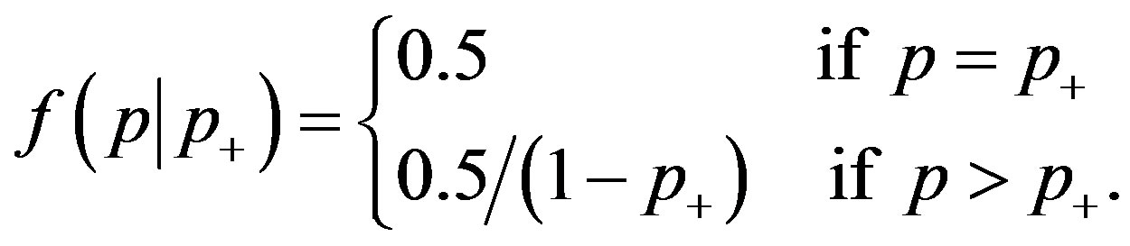
Then, p = 0 if and only if p = p₊, and under the null hypothesis p_– does not explicitly enter the calculations. To test the null hypothesis, create the prior distribution of p with mixed discrete and continuous parts

(1)

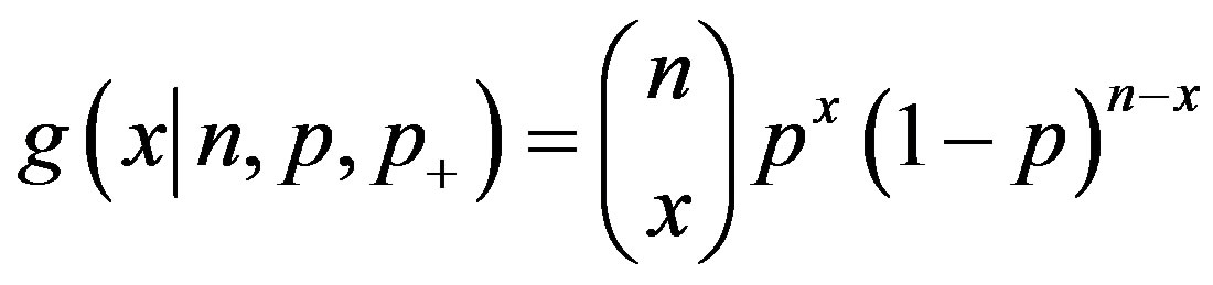
This prior distribution has been characterized as “virtually mandatory” [4, p. 151]. It gives probability 0.5 to each hypothesis with an uninformative uniform distribution covering the alternative hypothesis. The distribution of X is the binomial probability mass function

.

Bayes’ theorem says that the posterior probability that the null hypothesis is true is

(2)

where

(3)

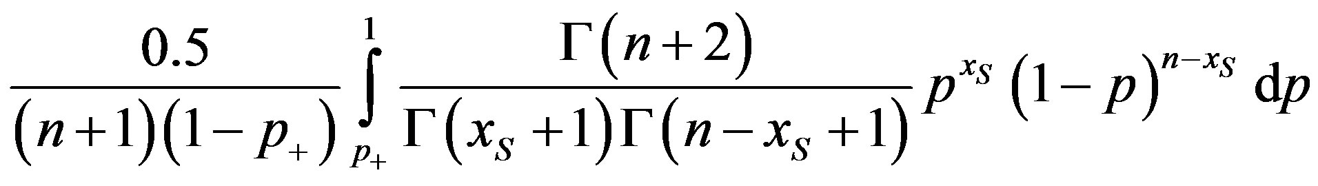
The integral in Equation (3) is

(4)

which is a constant times a probability computed from a beta distribution [4, p. 560], [5, pp. 33 and 48]. Decide in favor of the hypothesis with the larger posterior probability.

For our second example, in a sample of 223 eleven-year-old children in Britain diagnosed with eczema, 3 were diagnosed with psoriasis [6]. For the false positive rate p₊ = 0.01 among eczema suffers, g(0.01, 0.01) and

overwhelmingly favoring the null hypothesis.

One choice that was made to create the test in Equations (2)-(4) is the prior distribution in Equation (1). Generally, the prior distribution’s impact on the analysis matters less and less as sample size is increased. Another choice was that p₊ has a fixed value. A more complicated analysis would place a distribution on this error rate and average it out by integrating over the now-variable p₊ [4,5]. This type of analysis is presented in the next section.

4. More Extensive Tests

In this section we analyze our third example using expanded frequentist and Bayesian tests.

A person who suffers from Generalized Anxiety Disorder is in an almost constant state of apprehension. The null hypothesis is that there is no one in the population of American university students with GAD. That says GAD, as defined in psychiatry, does not exist in that population. Szasz [7] and others argue against the existence of such diseases. A study reported in [8] had a sample size n = 2843 students with 111 diagnosed with GAD. A misdiagnosis rate p₊ = 0.03 for GAD was reported by [9] and used in [8].

For the frequentist test with the 0.05 level of significance, the critical value is

.

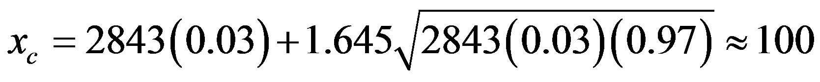Since 111 > 100, we conclude that this condition exists in this population. Alternatively, based on various sources [8-10], we might have supposed that the misdiagnosis rate is in the interval 0.01 ≤ p₊ ≤ 0.03. The critical values for p₊ = 0.01 and p₊ = 0.03 are 37 and 100, respectively, leading to the same conclusion.

For this example, we perform a more extensive Bayesian analysis, which uses simulation and a beta distribution for the hyper parameter p₊. Suppose we feel that p₊ follows a beta distribution with mean 0.02 and standard deviation 0.005. The mean is the center of the interval 0.01 ≤ p₊ ≤ 0.03, and the standard deviation is one-fourth the width of the interval. The mean and standard deviation uniquely determine the beta distribution’s parameters [2, p. 420].

We use a direct sampling approach to estimate P(p = 0 | X_s = 111) by averaging out the misclassification rates. To do this, perform m simulations of the misclassification rate p₊ from its beta distribution. For each simulated value p_+,k, calculate (0.5)g(p_+,k, p_+,k) and h(2843, p_+,k) for k = 1, 2, ..., m. The estimate of P(p = 0 | X_s = 111) is

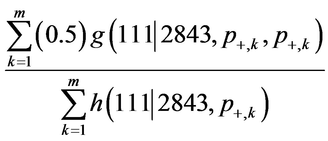
[4,5]. Using m = 20,000, a simulation yielded the estimate 0.4545 for P(p = 0 | X_s = 111). We reject the null hypothesis, which is consistent with the results from the frequentist test.

Sometimes, the frequentist and the Bayesian tests do not reach the same conclusion. In this example, if we know that the false positive rate is actually 0.03, then for the Bayesian test

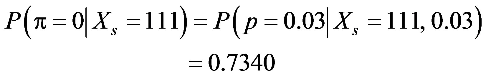
yielding a conclusion that instead strongly favors the null hypothesis. This potential difference in the conclusions is called Lindley’s paradox [4, p. 156], [5, p. 80].

REFERENCES

- R. V. Hogg, J. W. McKean and A. T. Craig, “Introduction to Mathematical Statistics,” 6th Edition, Pearson Prentice Hall, Upper Saddle River, 2005.
- V. K. Rohatgi, “Statistical Inference,” Dover, Mineola, 2003.
- D. C. Hooper, S. Spitsin, R. B. Kean, J. M. Champion, G. M. Dickson, I. Chaudhry and H. Koprowski, “Uric Acid, a Natural Scavenger of Peroxynitrite, in Experimental Allergic Encephalomyelitis and Multiple Sclerosis,” Proceedings of the National Academy of Science, USA, Vol. 95, No. 2, 1998, pp. 675-680. doi:10.1073/pnas.95.2.675
- J. O. Berger, “Statistical Decision Theory and Bayesian Analysis,” 2nd Edition, Springer, New York, 2010.
- K. R. Koch, “Introduction to Bayesian Statistics,” 2nd Edition, Springer, Berlin, 2010.
- H. C. Williams and D. P. Strachan, “Psoriasis and Eczema are not Mutually Exclusive Diseases,” Dermatology, Vol. 189, No. 3, 1994, pp. 238-240. doi:10.1159/000246845
- T. S. Szasz, “The Myth of Mental Illness,” In: A. L. Caplan, J. J. McCartney and D. A. Sisti, Eds., Health, Disease, and Illness: Concepts in Medicine, Georgetown University Press, Washington DC, 2004, pp. 43-50.
- D. Eisenberg, S. E. Gollust, E. Golberstein and J. L. Hefner, “Prevalence and Correlates of Depression, Anxiety, and Suicidality among University Students,” American Journal of Orthopsychiatry, Vol. 77, No. 4, 2007, pp. 534-542. doi:10.1037/0002-9432.77.4.534
- R. L. Spitzer, K. Kroenke, J. B. W. Williams and The Patient Health Questionnaire Primary Care Group, “Validation and Utility of a Self-Report Version of PRIMEMD: The PHQ Primary Care Study,” Journal of the American Medical Association, Vol. 282, No. 18, 1999, pp. 1737-1744. doi:10.1001/jama.282.18.1737
- S. Becker, K. Al Zaid and E. Al Faris, “Screening for Somatization and Depression in Saudi Arabia: A Validation Study of the PHQ in Primary Care,” International Journal of Psychiatric Medicine, Vol. 32, No. 3, 2002, pp. 271-283.