Open Journal of Statistics
Vol.3 No.2(2013), Article ID:30323,15 pages DOI:10.4236/ojs.2013.32012
Minimum Description Length Methods in Bayesian Model Selection: Some Applications
Statistics and Mathematics Unit, Indian Statistical Institute, Bangalore, India
Email: mohan.delampady@gmail.com
Copyright © 2013 Mohan Delampady. This is an open access article distributed under the Creative Commons Attribution License, which permits unrestricted use, distribution, and reproduction in any medium, provided the original work is properly cited.
Received January 8, 2013; revised February 10, 2013; accepted February 26, 2013
Keywords: Bayesian Analysis; Model Selection; Minimum Description Length; Hierarchical Bayes; Bayesian Computations
ABSTRACT
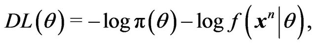
Computations involved in Bayesian approach to practical model selection problems are usually very difficult. Computational simplifications are sometimes possible, but are not generally applicable. There is a large literature available on a methodology based on information theory called Minimum Description Length (MDL). It is described here how many of these techniques are either directly Bayesian in nature, or are very good objective approximations to Bayesian solutions. First, connections between the Bayesian approach and MDL are theoretically explored; thereafter a few illustrations are provided to describe how MDL can give useful computational simplifications.
1. Introduction
Bayesian computations can be difficult, in particular those in model selection problems. For instance, it may be noted that learning the structure of Bayesian networks is in general of the computational complexity type NPcomplete ([1,2]). It is therefore meaningful to consider alternative computationally simpler solutions which are approximations to Bayesian solutions. Sometimes direct computational simplifications are possible, as shown, for example, in [3], but often approaches arising out of different methodologies are needed. We discuss some aspects of Minimum Description Length (MDL) methods with this point of view. Another important reason for exploring these methods is that there is a substantial literature on this topic available in engineering and computer science with potential applications in statistics. We will not, however, explore certain other aspects of MDL such as the “Normalized Maximum Likelihood (NML)” introduced by [4] which do not seem to be in the spirit of the Bayesian approach that we have taken here.
The discussion below is organized as follows. In Section 2 we briefly describe the MDL principle and then indicate in Sections 3 and 4 how it applies to model fitting and model checking. It is shown that a particular version of MDL is equivalent to the Bayes factor criterion of model selection. Since this is computationally difficult most often, some approximations are desirable, and it is next shown how a different version of MDL can provide such an approximation. Following this discussion, new applications are presented in Section 5. Specifically, MDL approach to step-wise regression in Section 5.1, wavelet thresholding in 5.2 and a change-point problem in 5.3 are described.
2. Minimum Description Length Principle
The MDL approach to model fitting can be described as follows (see [5,6]). Suppose we have some data. Consider a collection of probability models for this set of data. A model provides a better fit if it can provide a more compact description for the data. In terms of coding, this means that according to MDL, the best model is the one which provides the shortest description length for the given data. The MDL approach as discussed here is also related to the Minimum Message Length (MML) approach of [7]. See [8,9] for connections to information theory and other related details.
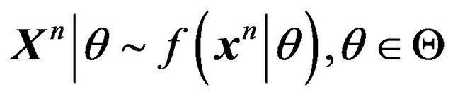
If data ![]() is known to arise from a probability density
is known to arise from a probability density![]() , then (see [10] or [11]) the optimal code length (in an average sense) is given by
, then (see [10] or [11]) the optimal code length (in an average sense) is given by . (Here
  is logaritm to the base 2.) This is the link between description length and model fitting.
The optimal code length of  is valid only in the discrete case. To handle the continuous case later, discretize x and denote it by
 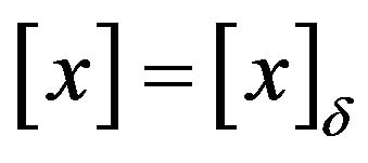 where
where ![]()
denotes the precision. In effect we will then be considering
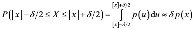
instead of  itself as far as coding of x is considered when x is one-dimensional. In the r-dimensional case, we will replace the density
  by the probability of the
  -dimensional cube of side
 ![]() containing
containing![]() , namely
, namely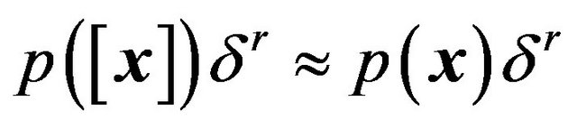 , so that the optimal code length changes to
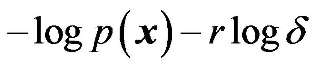 .
.
3. MDL for Estimation or Model Fitting
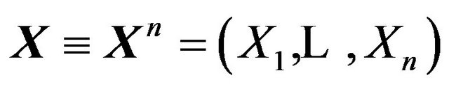
Consider data , and suppose
is the collection of models of interest. Further, let  be a prior density for
 . Given a value of
  (or a model), the optimal code length for describing
  is
is , but since
  is unknown, its description requires a further
  bits on average. Therefore the optimal code length is obtained upon minimizing
 (1)
(1)
so that MDL amounts to seeking that model which minimizes the sum of
• the length, in bits, of the description of the model, and
• the length, in bits, of data when encoded with the help of the model.
Now note that the posterior density of  given the data
  is
is
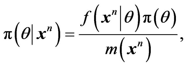 (2)
(2)
where 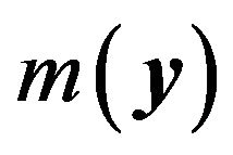 is the marginal or predictive density. Therefore, minimizing
over  is equivalent to maximizing
 . Thus MDL for estimation or model fitting is equivalent to finding the highest posterior density (HPD) estimate of
 . Note, however, that a prior
 ![]() is needed for these calculations. The approach that a Bayesian adopts in specifying the prior is not, in general, what is accepted by practitioners of the MDL approach. Therefore, the equivalence of MDL and HPD approaches is either subject to accepting the same prior, or as an asymptotic or similar approximation. MDL mostly prefers an approximately uniform prior when
is needed for these calculations. The approach that a Bayesian adopts in specifying the prior is not, in general, what is accepted by practitioners of the MDL approach. Therefore, the equivalence of MDL and HPD approaches is either subject to accepting the same prior, or as an asymptotic or similar approximation. MDL mostly prefers an approximately uniform prior when  for some fixed
  (same
(same  across all models), leading to the maximum likelihood estimate (MLE). The case of
  having model parameters of different dimensions is different and is interesting. This can be easily seen in the continuous case upon discretization. Now denote
  by
by  and
and  by
by . Then
Here  and
and  are the precisions required to discretize
 ![]() and
and , respectively. Note that the term
  is common across all models, so it can be ignored. However, the term
  which involves the dimension of
  in the model varies and is influential. According to [6,12],
  is optimal (see [13] for details), in which case
 (3)
(3)
Minimizing this will not lead to MLE even when π(θk) is assumed to be approximately constant. In fact, [12] proceeds further and argues that the correct precision  should depend on the Fisher information matrix. This amounts to using a prior which is similar in nature to the Jeffreys’ prior on
 . Jeffreys prior is an objective choice and thus this approach to MDL can then be considered a default Bayesian approach.
In spite of these desirable properties, however, MDL leads to the HPD estimate of , which is not the usual Bayes estimate. Posterior mean is what is generally preferred, so that the error in estimation has an immediate simple answer in the posterior standard deviation. In summary, therefore, the Bayesian approach doesn’t seem to find attractive solutions in the MDL approach as far as estimation or model fitting is concerned unless the models under consideration are hierarchical having parameters of varying dimension. On the other hand, when such hierarchical models are of interest the inference problem usually involves model selection in addition to model fitting. Thus the possible gains from studying the MDL approach are in the context of model selection as described below.
4. Model Selection Using MDL
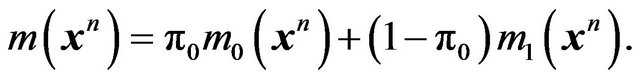
Let us recall the Bayesian approach to model selection and express it in the following form. Let
 . Suppose
 . Consider testing
 (4)
(4)
where , for some
 and
and . Let
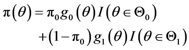
. Let ![]() be a prior on
be a prior on . Then
 ![]() can be expressed as
can be expressed as
 (5)
(5)
where  and
and  and
and  are the conditional densities (with respect to some dominating
 ![]() - finite measure) of
- finite measure) of  under
under  and
and  respectively. Then
 (6)
(6)
 (7)
(7)
where
 (8)
(8)
and
 (9)
(9)
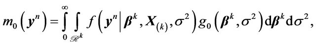
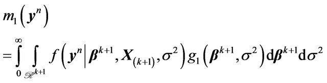
Note that  is simply the marginal or predictive density of
  under
under  and
and ![]() is the unconditional predictive density obtained upon averaging
is the unconditional predictive density obtained upon averaging  and
and . Consequently, the posterior odds ratio of
  relative to
  is,
is,
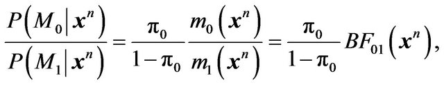 (10)
(10)
with  denoting the Bayes factor of
  relative to
 . When we compare two competing models
  and
and , we usually take
 , and hence settle upon the Bayes factor
  as the model selection tool. This agrees well with the intuitive notion that the model yielding a better predictive ability must be a better model for the given data.
4.1. Mixture MDL and Stochastic Complexity
Let us consider the MDL principle now for model selection between  and
and . Once the conditional prior densities
  and
and  are agreed upon, MDL will select that model
  which obtains a smaller value for the code length,
  , between the two. This is clearly equivalent to using Bayes factor as the model selection tool, and hence this version of MDL is equivalent to the Bayes factor criterion. In the MDL literature, this version of MDL is known as “mixture MDL”, and is distinguished from the “two-stage MDL” which separately codes the model and the prior. The two-stage MDL can be derived as an approximation to the mixture MDL as discussed later. See [13] for further details and other interesting comparisons and discussion. Let us consider a few examples before examining the need for other versions of MDL.
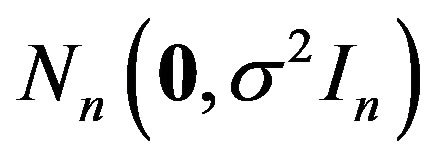
Example 1. Suppose Xn is a random sample from
 with known
 . We want to test

Consider the  prior on
  with known
  under
under . Then the marginal distribution of
  is
is
 under
under  and under
  it is
it is
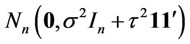 . A continuous model and a continuous prior is considered here. Since the precision of the prior parameter is the same across all models upon discretization we will ignore the distinction and proceed with densities. Then, both the Bayes factor criterion and the MDL principle will select
  over
over  if and only if
where  and
and  are the corresponding densities. Since we are comparing two logarithms, let us switch to natural logarithms. Then
 and
and
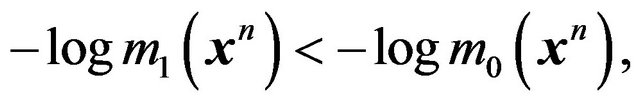
Noting that

and
we obtain
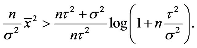
Therefore  is preferred over
  either by the Bayes factor or by the mixture MDL if and only if
Example 2. Let us consider the previous example with unknown  now. Suppose the prior on
  is the default
  under both models. The prior on
  under
under  is now assumed to depend on
 , i.e.,
 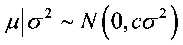 , where
  is assumed to be a known constant for now. Then, provided
 ,
,

and letting , and
, and  denote the marginal density of
  given
given ![]() and
and ,
,
Thus
Therefore, the Bayes factor criterion or the mixture MDL reduces to a criterion which is very similar to that given in the previous example, except that  is now replaced by an estimator.
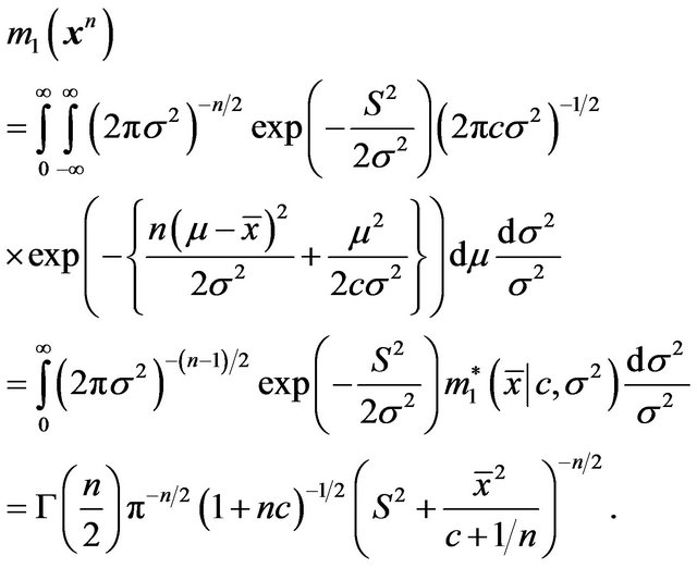
Example 3. (Jeffreys’ Test) This is similar to the problem discussed above, except that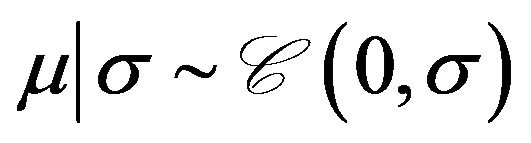 , with density
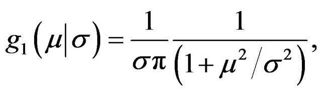
the Cauchy prior. The prior on ![]() is the same as before under both models:
is the same as before under both models: . This approach suggested by Jeffreys ([14]) is important. It explains how one should proceed when the hypotheses which describe the model selection problem involve only some of the parameters and the remaining parameters are considered to be nuisance parameters. Then Jeffreys suggestion is to employ the same noninformative prior on the nuisance parameters under both models, and a proper prior with low level of information on the parameters of interest. Details on this problem along with this choice of prior can be found in Section 2.7 of [15].
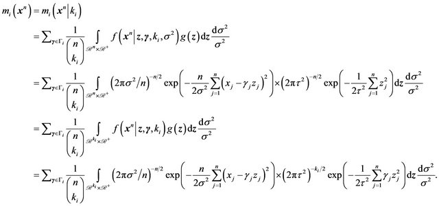
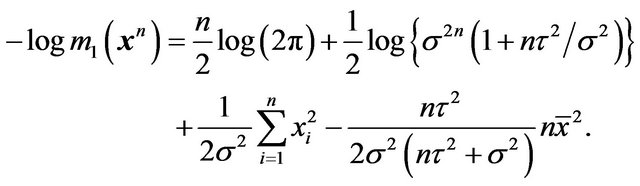
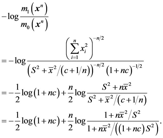
Note that  is the same as in the previous example, namely
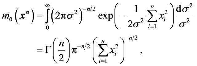
whereas
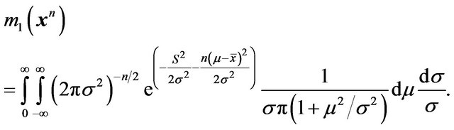
No closed form is available for m1(xn) in this case. To calculate this one can proceed as follows as indicated in Section 2.7 of [15]. The Cauchy density  can be expressed as a Gamma scale mixture of normals,
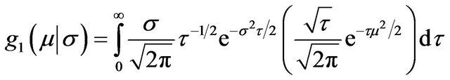
where ![]() is the mixing Gamma variable. Now one can integrate over
is the mixing Gamma variable. Now one can integrate over  and
and ![]() in closed form to simplify (m1xn). Finally, one has a one-dimensional integral over
in closed form to simplify (m1xn). Finally, one has a one-dimensional integral over ![]() left, which can be numerically computed whenever needed.
left, which can be numerically computed whenever needed.
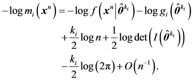
Now, let us note from the examples discussed above that an efficient computation of mi(xn) relies on having an explicit functional form for it. This is generally possible only when a conjugate prior is used as in Examples 1 and 2. For other priors, such as in Example 3, some numerical approximation will have to be employed. Thus we are lead to considering possible approximations to the mixture MDL technique, or equivalently to the Bayes factor, .
.
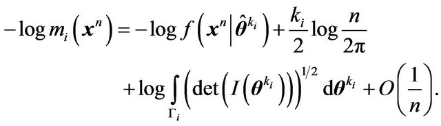
From Sections 4.3.1 and 7.1 of [15], assuming that  and
and  are smooth functions, we obtain, for large
![]() , the following asymptotic approximation for
, the following asymptotic approximation for  of equation (8). Let
 ![]() be the dimension of
be the dimension of ,
,
 and
and  denote the Hessian of
 , i.e.,
Also, let  denote either the MLE or the posterior mode. Then
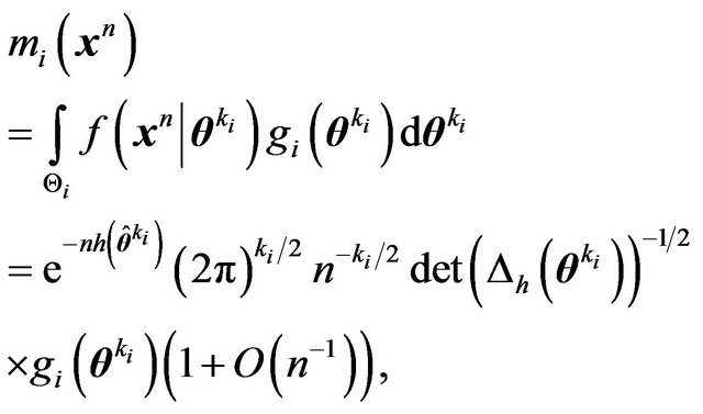 (11)
(11)
so that
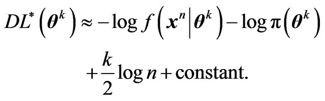
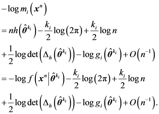 (12)
(12)
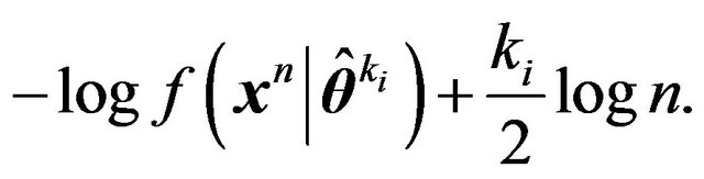
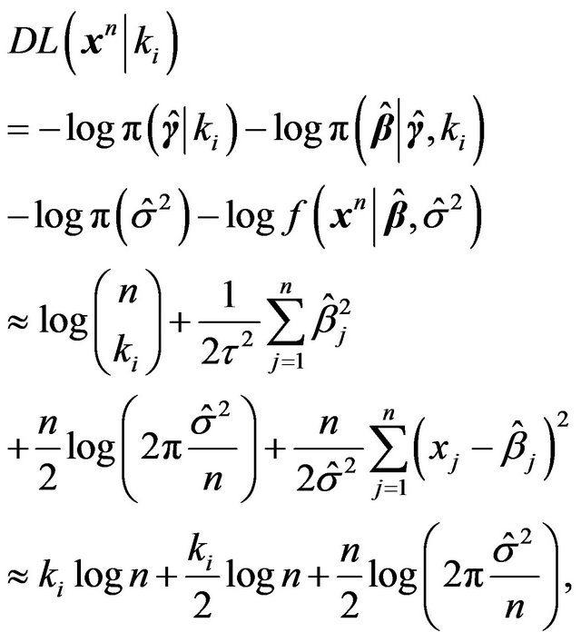
Ignoring terms that stay bounded as![]() , [12] suggests using the (approximate) criterion which Rissanen calls stochastic information complexity (or “stochastic complexity” for short),
, [12] suggests using the (approximate) criterion which Rissanen calls stochastic information complexity (or “stochastic complexity” for short),
 (13)
(13)
where
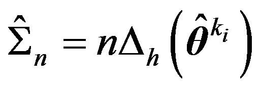 (14)
(14)
for implementing MDL. See [12,16-18] for further details.
If  are i.i.d. observations, then we have

where  is the Fisher Information matrix and hence
 (15)
(15)
Now ignoring terms that stay bounded as![]() , we obtain the Schwarz criterion ([19]), BIC, for
, we obtain the Schwarz criterion ([19]), BIC, for  given by
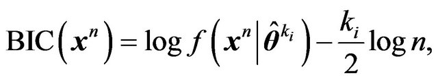 (16)
(16)
which can be seen to be asymptotically equivalent to SIC.
Example 4. [20] discusses a model selection problem for failure time data. The two models considered are exponential and Weibull:
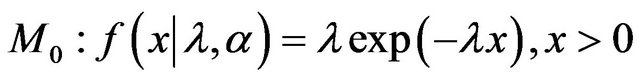
versus
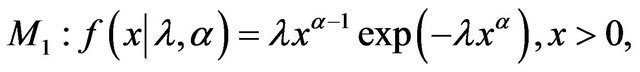
where  and
and . Model selection criterion of Rissanen is SIC as described in Equations (13) and (14). However, in this problem a better approximation is employed for the mixture MDL, the mixture being Jeffreys mixture, i.e., the conditional prior densities under
  for
for  are given by
where  is a compact subset of the relevant parameter space
  and
and . Consequentlyit follows that,

where  is the MLE of
  under
under . This yields,
Compare this with (15) and note that the term involving  vanishes.
We would like to note here that many authors [21,22] define the MDL estimate to be the same as the HPD estimate with respect to the Jeffreys’ prior restricted to some compact set  where its integral is finite:
which is the stochastic complexity approach advocated above.
It must be emphasized that proper priors are being employed to derive the SIC criterion, and hence indeterminacy and inconsistency problems faced by techniques employing improper priors are not a difficulty in this approach. Moreover, this approach can be viewed as an implementable approximation to an objective Bayesian solution.
4.2. Two-Stage MDL
Now consider the two-stage MDL which codes the prior and the likelihood separately and adds the two description lengths. This approach is therefore similar to estimating the parameter  with the HPD estimate when there is an informative prior, or with the MLE, but the resulting minimum description length does have interesting features. To see when and how this approach approximates the above mentioned model selection criterion, let us look at some of the specific details in the two stages of coding. See [12,13] for further details. Again, recall the setup in (4) and (5).
Stage 1. Let  be an estimate of
  such as the posterior mean, HPD or MLE under
 . This needs to be coded. Consider the prior density
  conditional on
  being true. Usually MDL would choose a uniform density. Restrict
  to a large compact subset of the parameter space and discretize it as discussed in Section 3 with a precision of
 . Then the codelength required for coding
  is
is
 (17)
(17)
Stage 2. Now the data  is coded using the model density
 . Discretization may again be neededsay with precision
 . Thus the description length for coding
  will be
 (18)
(18)
Summing these two codelengths, therefore, we obtain a total description length of
 (19)
(19)
Since the second term above,  , is constant over both M0 and
 , and the third term stays bounded as
 ![]() increases, these two terms are dropped from the MDL two-stage coding criterion. Thus, for regular parametric models, the two-stage MDL simplifies to the same criterion (for
increases, these two terms are dropped from the MDL two-stage coding criterion. Thus, for regular parametric models, the two-stage MDL simplifies to the same criterion (for ) as BIC, namely,
 (20)
(20)
In more complicated model selection problems, the two-stage MDL will involve further steps and may differ from BIC.
It may also be seen upon comparing (19) with (15) that the performance of SIC based MDL should be superior to the simplified two-stage MDL for moderate ![]() since SIC uses a better precision for coding the parameter, namely, one based on the Fisher information.
since SIC uses a better precision for coding the parameter, namely, one based on the Fisher information.
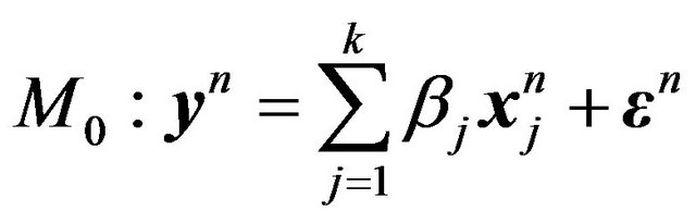
5. Regression and Function Estimation
Model selection is an important part of parametric and nonparametric regression and smoothing. Variable selection problems in multiple linear regression, order of the spline to fit and wavelet thresholding are some such areas. We will briefly consider these problems to see how MDL methods can provide computationally attractive approximations to the respective Bayesian solutions.
5.1. Variable Selection in Linear Regression
Variable selection is an important and well studied problem in the context of normal linear models. Literature includes [23-32]. We will only touch upon this area with the specific intention of examining useful and computationally attractive approximations to some of the Bayesian methods.
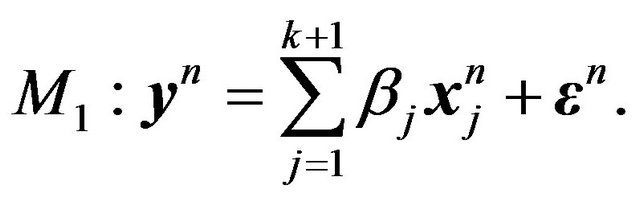
Suppose we have an observation vector yn on a response variable Y and also measurements  on a set of potential explanatory variables (or regressors). Following [13], we associate with each regressor
 , a binary variable
 . Then the set of available linear models is
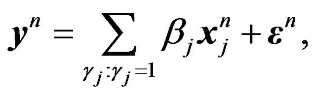 (21)
(21)
where . Note that
 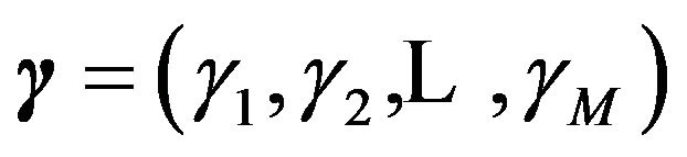 is, then, a Bernoulli sequence associated with the set of regression coefficients,
  also. Let
  denote the vector of non-zero regression coefficients corresponding to
 , and
, and  the corresponding design matrix, which results in the model
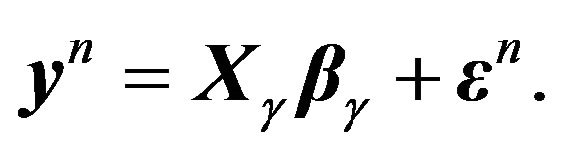
Selecting the best model, then, is actually an estimation problem, i.e., find the HPD estimate of  starting with a prior
  on
on  and a prior
  on
on  given
given . The two-stage MDL, which is the simplest, uses the criterion of minimizing
 (22)
(22)
MLE for  and
and  given
given  are easily available:
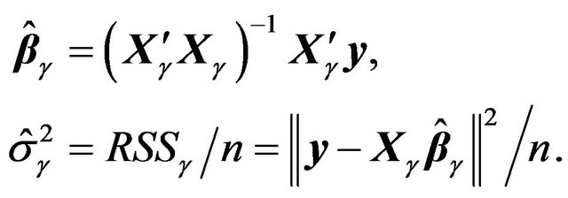 (23)
(23)
Consider the uniform prior on , all
, all  values receiving the same weight
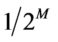 . Using these, we can re-write the MDL criterion as the one which minimizes (as in Example 2)
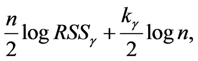 (24)
(24)
where  is the number of
 .
.
We can also derive the mixture MDL or stochastic complexity of a given model . If
. If  is the prior density under
 ,
,
 (25)
(25)
Applying (13), (14) after evaluating the information matrix of the parameters  and ignoring terms that are irrelevant for model selection, one obtains (see [13]),
 (26)
(26)
If ![]() is chosen to be the conjugate prior density, then the marginal density
is chosen to be the conjugate prior density, then the marginal density  can be explicitly derived. Details on this and further simplifications obtained upon using Zellner’s g-prior can be found in [13]. (See also [33,34].)
This method is only useful if one is interested in comparing a few of these models, arising out of some pre-specified subsets. Comparing all  models is not a computationally viable option for even moderate values of
 , since for each model,
  , one has to compute the corresponding
  and
and .
.
We are more interested in a different problem, namely, whether an extra regressor should be added to an already determined model. This is the idea behind the step-wise regression, forward selection method. In this set-up, the model comparison problem can be stated as comparing
versus
This is actually a model building method, so we assume that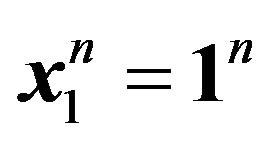 , and hence
 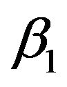 is the intercept which gives the starting model. Then we decide whether this model needs to be expanded by adding additional regressors. Thus, at step
 , we have an existing model with regressors
 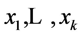 and we fix
  to be one of the remaining
  regressors as the candidate for possible selection. Now the two-stage MDL approach is straight forward. From (22) and (24), we note that
  is to be selected if and only if
 (27)
(27)
where  is the description length of the model with regressors
  and
and  is its residual sum of squares as given in (23). A closer look at (27) reveals certain interesting facts. We need the following additional notations involving design matrices and the corresponding projection matrices. We assume that the required matrix inverses exist.
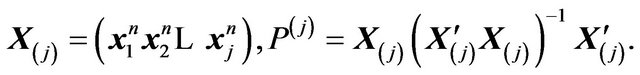
Then we note the following result which may be found, for example, in [35].
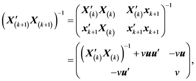 (28)
(28)
where
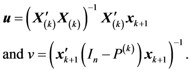
It then follows that
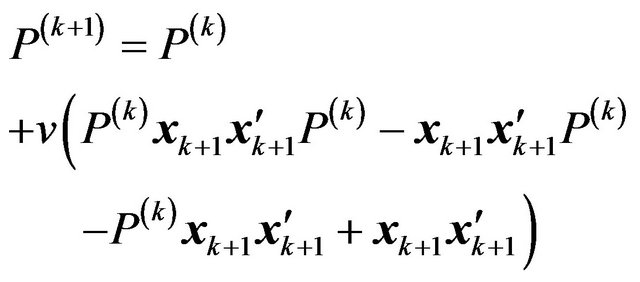
and hence
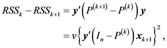
and
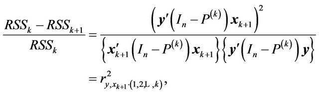
where 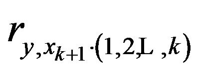 is simply the partial correlation coefficient between
 ![]() and
and  conditional on
 . Substituting these in (27), we see that
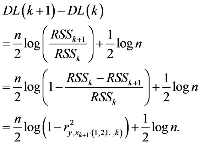 (29)
(29)
Therefore,
 if and only if
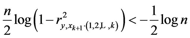 if and only if
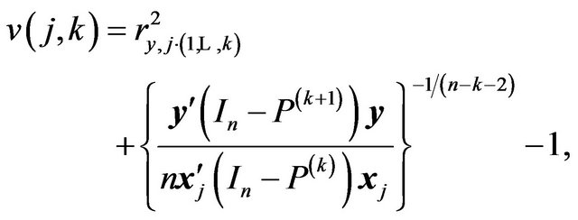
![]() (30)
(30)
This method does have some appeal, in that at each step, it tries to select that variable which has the largest partial correlation with the response (conditional on the variables which are already in the model), just like the step-wise regression method. However, unlike the stepwise regression method it does not require any stopping rule to decide whether the candidate should be added. It relies on the magnitude of the partial correlation instead.
One can also apply the stochastic complexity criterion given in (26) above. Then we obtain,
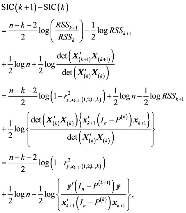
(31)
which is related to the step-wise regression approach, but uses more information than just the partial correlation.
A full-fledged Bayesian approach using the g-prior can also be implemented as shown below. Note that
and
 (32)
(32)
where  and
and , respectively, are the prior densities under
  and
and . Taking these priors to be g-priors, namely,
along with the density  for
for , a (proper prior) density
  for the hyperparameter
![]() , we obtain,
, we obtain,
 (33)
(33)
where
 (34)
(34)
with  and
and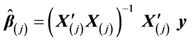 .
.
The one-dimensional integrals in (33), however, cannot be obtained in closed form. One could also approximate
 with
with , where
  are the ML-II (cf. [36]) estimates of
![]() . See [13] for details.
. See [13] for details.
Example 5. We illustrate the MDL approach to stepwise regression by applying it to the Iowa-corn-yielddata (see [37,38]). We have not included “year” as a regressor (which is a proxy for technological advance) and instead have considered only the weather-related regressors.
In this data set the variables are: X1 = Year, 1 denoting 1930, X2 = Pre-season precipitation, X3 = May temperature, X4 = June rain, X5 = June temperature, X6 = July rain, X7 = July temperature, X8 = August rain, X9 = August temperature, and Y = X10 = Corn Yield.
As mentioned earlier, we always keep the intercept and check whether this regression should be enlarged by adding more regressors. We first apply the Two-stage MDL criterion. From (30), at step , we consider only those regressors (which are not already in the model and)
which satisfy ![]() (=0.1005 in this example). From this set we pick the one with the largest
(=0.1005 in this example). From this set we pick the one with the largest
![]() . The values of
. The values of ![]() for the relevant steps are listed below.
for the relevant steps are listed below.
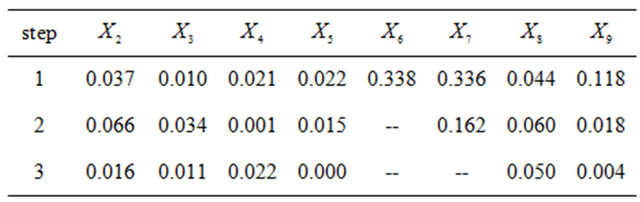
According to our procedure we select  first, followed by
  and the selection ends there.
We consider the SIC criterion next. From (31), at step , we pick the regressor
  with the largest value for
provided it is positive. The values of  for the relevant steps are given below.
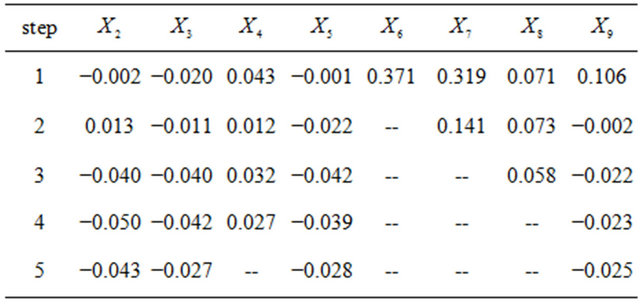
According to SIC our order of selection is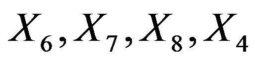 .
.
5.2. Wavelet Thresholding
Consider the nonparametric regression problem where we have the following model for the noisy observations :
:
 (35)
(35)
where ![]() are i.i.d.
are i.i.d.  errors with unknown error variance
 , and
, and ![]() is a function (or signal) defined on some interval
is a function (or signal) defined on some interval . Assuming s is a smooth function satisfying certain regularities (see [15,39,40]), we have the wavelet decomposition of
![]() :
:
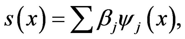 (36)
(36)
where  are the wavelet functions and
 is the corresponding vector of wavelet coefficients. We assume that the normally infinite sum in (36) can be taken to be a finite sum (or at least a very good approximation) as indicated in [39].
Upon applying the discrete wavelet transform (DWT) to![]() , we get the estimated wavelet coefficients,
, we get the estimated wavelet coefficients, . Consider now the equivalent model:
where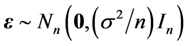 .
.
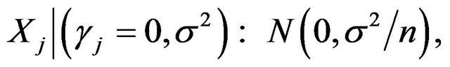
The model selection problem here involves determining the number of non-zero wavelet coefficients:
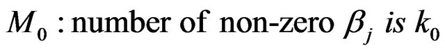
versus
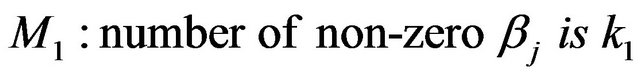
where  are the number of wavelet coefficients of interest.
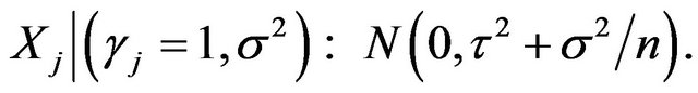
The prior distribution on the non-zero  is assumed to be i.i.d.
  under
under .
.
Since we have not identified the locations (indices) of the non-zero wavelet coefficients,  , we proceed as follows to describe the prior structure. With each
  we associate a binary variable
  as in [41] for wavelet regression or as in [13] for variable selection in regression. Then
  is a Bernoulli sequence associated with the set of regression coefficients,
 . Let
. Let
Finally, we let  be i.i.d.
  (
(![]() be the corresponding joint density), and define the following structure under
be the corresponding joint density), and define the following structure under .
.
 (37)
(37)
 (38)
(38)
 (39)
(39)
The nuisance parameter  which is common under both models is given the prior density
 . Then it follows that
 (40)
(40)
Note that only those  for which
  appear in the integral above.
The Two-stage MDL approach is clearly the easiest to take in this problem. As described earlier, it approximates  by coding the prior and the likelihood (both evaluated at an estimate) separately and sums the codelengths to obtain the description length. In this case, discretizing
  and
and  to a precision of
  and ignoring terms that stay bounded as
 ![]() increases, this amounts to
increases, this amounts to
 (41)
(41)
where the first term is obtained from Stirling’s approximation, the second term 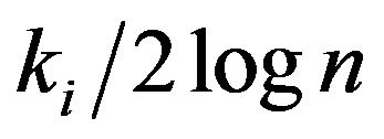 is for coding the
 ![]() non-zero
non-zero ’s and
 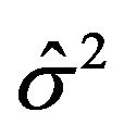 is an estimate such as the MLE. On the other hand, computing SIC or
  is not an impossible task either. In fact, to integrate out the
  in
in 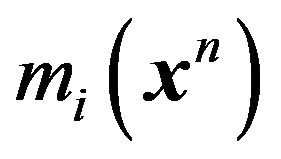 of Equation (40) we argue as follows.
 and
and
Now, as we argued in Jeffreys test, we take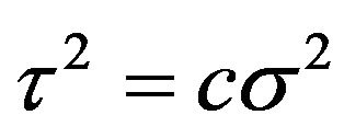 , and integrate out
  also. This leaves us with the following expression where we have a sum over
 .
.
 (42)
(42)
The term  is interesting. Most of the contribution to this sum is expected from
  with
with  corresponding to the largest
 ![]() of the
of the , which yields the MLE of
  upon normalization. The Bayes estimate, on the other hand, will arise from a weighted average of all the sums, with weights depending on the posterior probabilities of the corresponding
 . As is clear, weighted average over the space
  is computationally very intensive when
 ![]() and
and ![]() are large. An appropriate approximation is indeed necessary, and MDL is important in that sense.
are large. An appropriate approximation is indeed necessary, and MDL is important in that sense.
Even though we have justified the two-stage MDL for wavelet thresholding by showing that it is an approximation to a mixture MDL corresponding to a certain prior, a few questions related to this prior remain. First of all, the prior assumption that  are i.i.d.
  is unreasonable; wavelet coefficients corresponding to wavelets at different levels of resolution must be modeled with different variances. Specifically they should decrease as the resolution level increases to indicate their decreasing importance (see [40,42,43]). Secondly, wavelet coefficients tend to cluster according to resolution levels (see [44]), so instead of independent normal priors, a multivariate normal prior with an appropriate dependence structure must be employed. These modifications can be easily implemented in the Bayesian approach, except that the resulting computational requirements may be substantial.
5.3. Change Point Problem
We shall now consider MDL methods for a problem which attempts to decide whether there is a change-point in a given time series data. We use the data on British road casualties available in [45], which examines the effects on casualty rates of the seat belt law introduced on 31 January 1983 in Great Britain.
We follow the approach of [46]. Let  be independent Poisson counts with
 .
.  are a priori considered related, and a joint multivariate normal prior distribution on their logarithm is assumed. Specifically, let
  be the
  th element of
 ![]() and suppose
and suppose
We model the change-point as the model selection problem:
versus
where  is the possible change-point. We further let
  be i.i.d.
 . Note that
  and
and  are hyperparameters.
First, we approximate the likelihood function assuming  as follows.
(43)
where . Expanding (43) about
 , its maximum, in Taylor series and ignoring higher order terms in
 , we obtain
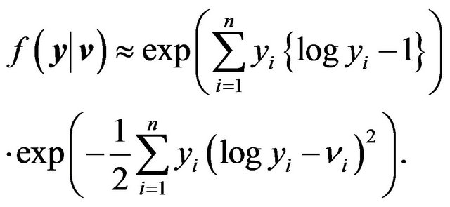 (44)
(44)
What is appealing and useful about (44) is that it is proportional to the multivariate normal likelihood function (for![]() ) with mean vector x and covariance matrix
) with mean vector x and covariance matrix  where
where
 and
and
Thus hierarchical Bayesian analysis of multivariate normal linear models is applicable (see [15,36,47]). We note that the hyper-parameters  and
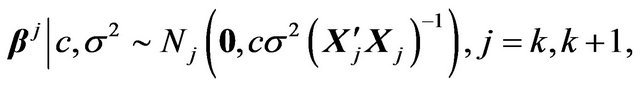
and  do not have substantial influence and hence treat them as fixed constants (to be chosen based on some sensitivity analysis) in the following discussion. Consequently, denoting by
  and
and  the respective prior densities under
  and
and ,
,
 (45)
(45)
Now, from multivariate normal theory, observe that
 (46)
(46)
and subsequently that,  can be integrated out as in Example 2. Thus,
 (47)
(47)
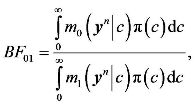
Expression (47) is not available, in general, in closed form. Approaching it from the MDL technique, we look for a subsequent approximation employing an ML-II type estimator (cf. [36]) for . Again, from (47), an ML-II likelihood for
  is given by
  which maximizes

For fixed  and
and  this involves only examining a smooth function of a single variable,
  , which is a simple computational task.
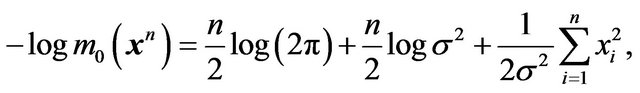
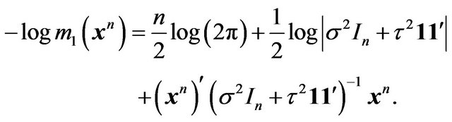
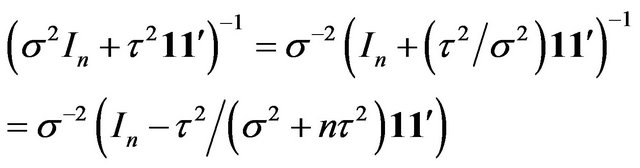
We proceed exactly as above to derive  also. Partition the required vectors and matrices as follows.
Then we have
(48)
 (a)
(a)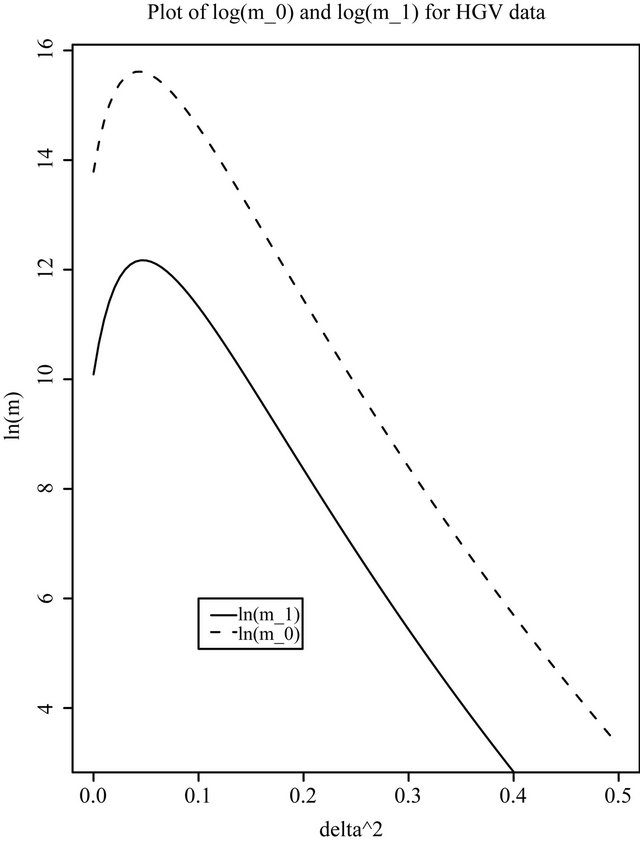 (b)
(b)
Figure 1. Plots of log(m0) and log(m1) for the British road casualties data. (a) LGV data; (b) HGV data.
As before, the MDL technique invloves deriving the ML-II estimator of  from
from , for fixed
  and
and . Obtaining
  (for fixed
  and
and
 ) which maximizes
  is very similar to that for
 .
.
We have applied this technique to analyze the British Road Casualties data. Figures 1(a) and (b) show
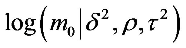 and
and 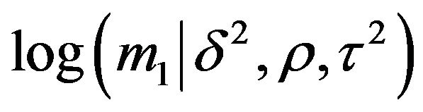 as a function of
  for
for  and
and , for the LGV and HGV data, respectively. As mentioned previously,
  and
and  do not seem to play any influential role; any reasonably small value of
  seems to yield similar results, and any
  which is not too close to 0 behaves similarly.
There seems to be strong evidence for a change-point in the intensity rate of casualties (induced by the ‘seatbelt law’) in the case of the LGV data, whereas this is absent in the case of the HGV data. This is evident from the very high value of  near the ML-II estimate of
  for the LGV data.
There is a vast literature related to MDL, mostly in engineering and computer science. See [48] and the references listed there for the latest developments. See also [49]. [50] provides a review of MDL and SIC, and claim that SIC is the solution to “optimal universal coding problems”. MDL techniques have not become very popular in statistics, but they seem to be quite useful in many applications.
REFERENCES
- N. B. Asadi, T. H. Meng and W. H. Wong, “Reconfigurable Computing for Learning Bayesian Networks,” Proceedings of 16th International ACM/SIGDA Symposium on Field Programmable Gate Arrays, Monterey, 24-26 February, 2008, pp. 203-211.
- D. M. Chickering, “Learning Bayesian Networks is NP- Complete,” In: D. Fisher and H.-J. Lenz, Eds., Learning from Data: AI and Statistics, V, Springer, Berlin, Heidelberg, New York, 1996, pp. 121-130.
- H. Younes, M. Delampady, B. MacGibbon and O. Cherkaoui, “A Hierarchical Bayesian Approach to the Estimation of Monotone Hazard Rates in the Random Censorship Model,” Journal of Statistical Research, Vol. 41, No. 2, 2007, pp. 35-42.
- Y. M. Shtarkov, “Universal Sequential Coding of Single Messages,” Problems of Information Transmission, Vol. 23, No. 3, 1987, pp. 3-17.
- J. Rissanen, “Modeling by Shortest Data Description,” Automatica, Vol. 14, No. 5, 1978, pp. 465-471. doi:10.1016/0005-1098(78)90005-5
- J. Rissanen, “A Universal Prior for Integers and Estimation by Minimum Description Length,” Annals of Statistics, Vol. 11, No. 2, 1983, pp. 416-431. doi:10.1214/aos/1176346150
- C. S. Wallace and P. R. Freeman, “Estimation and Inference by Compact Coding (with Discussion),” Journal of the Royal Statistical Society, Vol. 49, No. 3, 1987, pp. 240-265.
- P. M. B. Vitanyi and M. Li, “Minimum Description Length Induction, Bayesianism, and Kolmogorov Complexity,” IEEE Transactions on Information Theory, Vol. 46, No. 2, 2000, pp. 446-464. doi:10.1109/18.825807
- M. Li and P. Vitanyi, “An Introduction to Kolmogorov Complexity and Its Applications,” 3rd Edition, Springer, Berlin, 2008. doi:10.1007/978-0-387-49820-1
- T. M. Cover and J. A. Thomas, “Elements of Information Theory,” Wiley, Hoboken, 2006.
- G. H. Choe, “Computational Ergodic Theory,” Springer, New York, 2005.
- J. Rissanen, “Stochastic Complexity and Statistical Inquiry,” World Scientific, Singapore, 1989.
- B. Yu and M. H. Hansen, “Model Selection and the Principle of Minimum Description Length,” Journal of the American Statistical Association, Vol. 96, No. 454, 2001, pp. 746-774. doi:10.1198/016214501753168398
- H. Jeffreys, “Theory of Probability,” 3rd Edition, Oxford University Press, New York, 1961.
- J. K. Ghosh, M. Delampady and T. Samanta, “An Introduction to Bayesian Analysis: Theory and Methods,” Springer, New York, 2006.
- J. Rissanen, “Stochastic Complexity and Modeling,” Annals of Statistics, Vol. 14, No. 3, 1986, pp. 1080-1100. doi:10.1214/aos/1176350051
- J. Rissanen, “Stochastic Complexity (with Discussion),” Journal of the Royal Statistical Society (Series B), Vol. 49, No. 3, 1987, pp. 223-265.
- J. Rissanen, “Fisher Information and Stochastic Complexity,” IEEE Transactions on Information Theory, Vol. 42, No. 1, 1996, pp. 48-54. doi:10.1109/18.481776
- G. Schwarz, “Estimating the Dimension of a Model,” Annals of Statistics, Vol. 6, No. 2, 1978, pp. 461-464. doi:10.1214/aos/1176344136
- J. Rissanen and G. Shedler, “Failure-Time Prediction,” Journal of Statistical Planning and Inference, Vol. 66, No. 2, 1998, pp. 193-210. doi:10.1016/S0378-3758(97)00083-9
- H. Matsuzoe, J. Takeuchi and S. Amari, “Equiaffine Structures on Statistical Manifolds and Bayesian Statistics,” Differential Geometry and Its Applications, Vol. 24, No. 6, 2006, pp. 567-578. doi:10.1016/j.difgeo.2006.02.003
- J. Takeuchi, “Characterization of the Bayes Estimator and the MDL Estimator for Exponential Eamilies,” IEEE Transactions on Information Theory, Vol. 43, No. 4, 1997, pp. 1165-1174. doi:10.1109/18.605579
- J. O. Berger and L. R. Pericchi, “The Intrinsic Bayes Factor for Linear Models (with Discussion),” In: J. M. Bernardo, et al., Eds., Bayesian Statistics, Oxford University Press, London, 1996, pp. 25-44.
- D. P. Foster and E. I. George, “The Risk Inflation Criterion for Multiple Regression,” Annals of Statistics, Vol. 22, No. 4, 1994, pp. 1947-1975. doi:10.1214/aos/1176325766
- D. P. Foster and R. A. Stine, “Local Asymptotic Coding and the Minimum Description Length,” IEEE Transactions on Information Theory, Vol. 45, No. 4, 1999, pp. 1289-1293. doi:10.1109/18.761287
- P. H. Garthwaite and J. M. Dickey, “Elicitation of Prior Distributions for Variable-selection Problems in Regression,” Annals of Statistics, Vol. 20, No. 4, 1992, pp. 1697-1719. doi:10.1214/aos/1176348886
- P. H. Garthwaite and J. M. Dickey, “Quantifying and Using Expert Opinion for Variable-Selection Problems in Regression (with Discussion),” Chemometrics and Intelligent Laboratory Systems, Vol. 35, No. 1, 1996, pp. 1-43. doi:10.1016/S0169-7439(96)00035-4
- E. I. George and D. P. Foster, “Calibration and Empirical Bayes Variable Selection,” Biometrika, Vol. 87, No. 4, 2000, pp. 731-747. doi:10.1093/biomet/87.4.731
- M. H. Hansen and B. Yu, “Bridging AIC and BIC: An MDL Model Selection Criterion,” Proceedings of the IT Workshop on Detection, Estimation, Classification and Imaging, Santa Fe, 24-26 February 1999, p. 63.
- T. J. Mitchell and J. J. Beauchamp, “Bayesian Variable Selection in Linear Regression (with Discussion),” Journal of the American Statistical Association, Vol. 83, No. 404, 1988, pp. 1023-1036. doi:10.1080/01621459.1988.10478694
- A. F. M. Smith and D. J. Spiegelhalter, “Bayes Factors and Choice Criteria for Linear Models,” Journal of the Royal Statistical Society, (Series B), Vol. 42, No. 2, 1980, pp. 213-220.
- A. Zellner and A. Siow, “Posterior Odds Ratios for Selected Regression Hypotheses,” In: J. M. Bernardo, et al., Eds., Bayesian Statistics, University Press, Valencia, 1980, pp. 585-603.
- A. Zellner, “Posterior Odds Ratios for Regression Hypotheses: General Considerations and Some Specific Results,” In: A. Zellner, Ed., Basic Issues in Econometrics, University of Chicago Press, Chicago, 1984, pp. 275-305.
- A. Zellner, “On Assessing Prior Distributions and Bayesian Regression Analysis With g-Prior Distributions,” In: P. K. Goel and A. Zellner, Eds., Basic Bayesian Inference and Decision Techniques: Essays in Honor of Bruno de Finetti, Amsterdam, 1986, pp. 233-243.
- G. A. F. Seber, “A Matrix Handbook for Statisticians,” Wiley, Hoboken, 2008, PMid: 19043372.
- J. O. Berger, “Statistical Decision Theory and Bayesian Analysis,” 2nd Edition, Springer-Verlag, New York, 1985. doi:10.1007/978-1-4757-4286-2
- L. A. Shaw and D. D. Durast, “Measuring the Effects of Weather on Agricultural Output,” ERS-72, US Department of Agriculture, Washington DC, 1962.
- L. M. Thompson, “Weather and Technology in the Production of Corn and Soybeans,” CAED Report 17, Iowa State University, Iowa, 1963.
- A. Antoniadis, I. Gijbels and G. Grégoire, “Model Selection Using Wavelet Decomposition and Applications,” Biometrika, Vol. 84, No. 4, 1997, pp. 751-763. doi:10.1093/biomet/84.4.751
- J.-F. Angers and M. Delampady, “Bayesian Nonparametric Regression Using Wavelets,” Sankhyā: The Indian Journal of Statistics, Vol. 63, No. 3, 2001, pp. 287-308.
- M. S. Crouse, R. D. Nowak and R. J. Baraniuk, “WaveletBased Signal Processing Using Hidden Markov Models,” IEEE Transactions on Signal Processing, Vol. 46, No. 4, 1998, pp. 886-902. doi:10.1109/78.668544
- F. Abramovich and T. Sapatinas, “Bayesian Approach to Wavelet Decomposition and Shrinkage,” In: P. Müller and B. Vidakovic, Eds., Bayesian Inference in WaveletBased Models: Lecture Notes in Statistics, Vol. 141, Springer, New York, 1999, pp. 33-50.
- B. Vidakovic, “Nonlinear Wavelet Shrinkage with Bayes Rules and Bayes Factors,” Journal of the American Statistical Association, Vol. 93, No. 441, 1998, pp. 173-179. doi:10.1080/01621459.1998.10474099
- T. C. M. Lee, “Tree-Based Wavelet Regression for Correlated Data Using the Minimum Description Principle,” Australian & New Zealand Journal of Statistics, Vol. 44, No. 1, 2002, pp. 23-39. doi:10.1111/1467-842X.00205
- A. C. Harvey and J. Durbin, “The Effects of Seat Belt Legislation on British Road Casualties: A Case Study in Structural Time Series Modelling (with Discussion),” Journal of the Royal Statistical Society (Series A), Vol. 149, No. 3, 1986, pp. 187-227. doi:10.2307/2981553
- M. Delampady, I. Yee and J. V. Zidek, “Hierarchical Bayesian Analysis of a Discrete Time Series of Poisson Counts,” Statistics and Computing, Vol. 3, No. 1, 1993, pp. 7-15. doi:10.1007/BF00146948
- D. V. Lindley and A. F. M. Smith, “Bayes Estimates for the Linear Model,” Journal of the Royal Statistical Society (Series B), Vol. 34, 1972, pp. 1-41.
- P. D. Grunwald, “The Minimum Description Length Principle,” MIT Press, Cambridge, Massachusetts, 2007.
- S. de Rooij and P. Grunwald, “An Empirical Study of Minimum Description Length Model Selection with Infinite Parametric Complexity,” Journal of Mathematical Psychology, Vol. 50, No. 2, 2006, pp. 180-192. doi:10.1016/j.jmp.2005.11.008
- A. Barron, J. Rissanen and B. Yu, “The Minimum Description Length Principle in Coding and Modeling,” IEEE Transactions on Information Theory, Vol. 44, No. 6, 1998, pp. 2743-2760. doi:10.1109/18.720554