ABSTRACT

When sampling from a finite population there is often auxiliary information available on unit level. Such information can be used to improve the estimation of the target parameter. We show that probability samples that are well spread in the auxiliary space are balanced, or approximately balanced, on the auxiliary variables. A consequence of this balancing effect is that the Horvitz-Thompson estimator will be a very good estimator for any target variable that can be well approximated by a Lipschitz continuous function of the auxiliary variables. Hence we give a theoretical motivation for use of well spread probability samples. Our conclusions imply that well spread samples, combined with the HorvitzThompson estimator, is a good strategy in a varsity of situations.

1. Introduction

In many fields there has been a great interest in selecting samples that are well spread or spatially balanced. Such samples are considered to produce good estimates for target variables that exhibit spatial trends, see e.g. [1,2]. The focus in this paper is to explain the connection between a well spread sample and a balanced sample. Roughly speaking, a sample is well spread if the number of selected units is close to what is expected on average, in every part of the auxiliary space. A sample is balanced on a variable if the Horvitz-Thompson (HT) estimator of the total of that variable agree exactly with the known population total of the variable. In fact, with a short analysis, this paper clarifies why a well spread sample is approximately balanced. We also explain that, if the sample is well spread, the variance of commonly used estimators is usually low.

It is well known that samples that are balanced or approximately balanced on the auxiliary variables may be selected by using the cube method, see e.g. [3]. Sampling methods for selection of well spread samples in a general auxiliary space, by utilizing a distance function, are more recent and less well known than the cube method. Two such methods are the local pivotal method (LPM) and spatially correlated Poisson sampling (SCPS). The LPM design, based on the pivotal method [4], was first introduced in [5]. The other method, SCPS, was first introduced in [6] and it is a special case of the method described in [7].

In many areas, such as forest inventories, environmental studies, and even in official statistics, different forms of stratification are commonly used to obtain samples that are well spread geographically or in other available information. Often, stratification is used as a variance reduction technique without particular interest in the different strata. Constructing a stratified sampling design is often not straightforward, especially if several mixed auxiliary variables are available. It is not uncommon that statisticians try to stratify using several variables, but crossing all strata of all variables usually results in cells that are too small. In such situations it may be preferable and less complicated to define a distance measure in the auxiliary space, and then use a sampling method that in general avoid selection of nearby units, thus forcing the sample to be well spread.

In Section 2, a theoretical motivation for the balancing effect of well spread samples is given. In Section 3, we give arguments indicating that using well spread samples provides a small anticipated variance for the HT-estimator under a very general super-population model. Some sampling methods for selecting well spread samples are briefly discussed in Section 4. Final comments are provided in Section 5.

2. Main Results

We start by introducing some notation and assumptions. Let be a population of N units. We wish to select a probability sample s of size n in order to estimate some characteristics of U. It is assumed that we have access to auxiliary information on unit level, i.e. the values of q auxiliary variables are known for each unit. We also assume that it is possible to calculate the distance between two units i and j in the auxiliary space. Usually the total

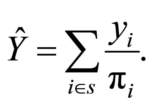
of one or more target variables are the parameters we wish to estimate. It is assumed that each population unit i is included in the sample with a known probability, , with, where n is the sample size. In this case the unbiased and commonly used HT-estimator [8] of Y is

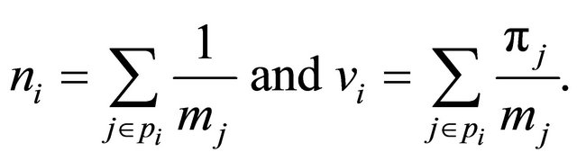
We are now ready to formalize what a well spread sample is. As suggested in [2], we use Voronoi polytopes to measure how well spread a sample is. The Voronoi polytope, for, includes all population units j satisfying for all sample units. Let n_i denote the number of units in p_i, with the correction that if a unit j is included in m_j polytopes, then j is counted as. Next, let v_i be the sum of the inclusion probabilities in p_i. Again, if a unit j is included in m_j polytopes, then its inclusion probability is divided equally to each of the m_j polytopes. Hence,

Note that and. We are now ready to give the definition of a well spread sample.

Definition 1 A sample is said to be well spread (or spatially balanced) with respect to the inclusion probabilities if each v_i is equal or close to 1.

As a measure of how well spread a sample is, we may use

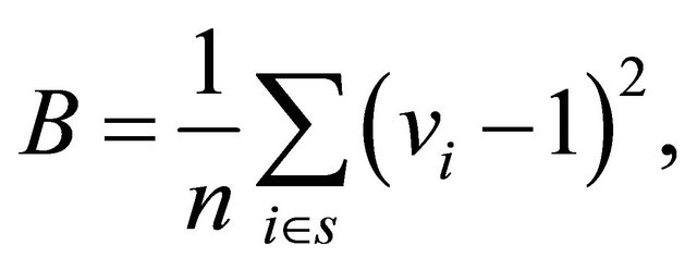(1)

see e.g. [2]. A small value of B indicates a very well spread sample. The mean of B over repeated samples is an indicator of how well spread samples a design produces. We next define a balanced and an approximately balanced sample.

Definition 2 We say that a sample s is balanced on the auxiliary x-variables if

Moreover, a sample is said to be approximately balanced if is close to.

In order to show that well spread samples are balanced we start by making three quite strong assumptions on the sample and the population. Later we will relax these assumptions a bit and then show that a larger class of well spread samples are approximately balanced. We first assume the following. 

(A.0) In each polytope the inclusion probabilities sum to 1, i.e.

(A.1) In each polytope the inclusion probabilities are equal, i.e. for every, we assume

(A.2) In each polytope the auxiliary variables are equal for all units, i.e. for every,

The assumptions (A.0) and (A.1) tell us that the size n_i of the polytope is equal to and (A.2) tells us that, for. Note that, and hence are allowed to vary between polytopes. Under the three assumptions it follows that

(2)

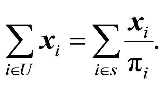
Thus the sample is balanced on any function and in particular, it is balanced on the auxiliary variables if we put.

The next step consists of introducing the following three new and less restrictive assumptions. 

For each polytope p_i, the inclusion probabilities satisfies

In each polytope, we have

The target is a Lipschitz continuous function of the auxiliary variables, i.e.

Remark 1 Concerning the validity of assumption, the inclusion probabilities are (if unequal) supposed to be derived from the auxiliary x-variables, perhaps they are chosen proportional to one of the x-variables, so they should not vary much within a polytope. Remember that the polytopes are constructed by grouping together units with similar x-values.

We are now ready to state and prove our main result.

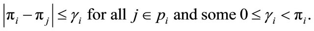
Theorem 1 Let be a well spread sample satisfying for all and for some. Assume also that is from a population satisfying assumptions. Then is approximately balanced. In particular,

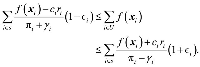
By sending we obtain exact balance on the target since

Note also that if we put then we get a balanced sample, see Definition 2. Besides that Theorem 1 tells us that when are small, the sample will be approximately balanced on and, it also gives bounds for the target parameter. We can however do better than the bounds in Theorem 1. For instance, we have

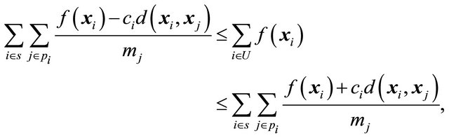
but these bounds are constructed by applying a worst case senario, within each polytope, so we cannot expect the bounds to be very good.

Proof of Theorem 1. By assumption and since 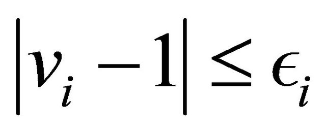we have, for all,

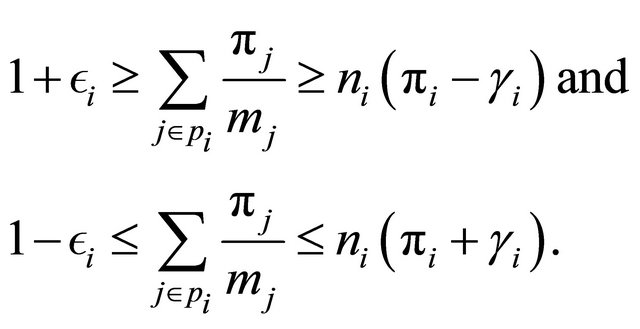(3)

The inequalities in (3) give

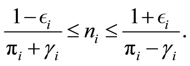(4)

Moreover, from assumptions and we see that

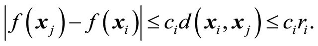(5)

Theorem 1 now follows from (4) and (5). In particular,

and

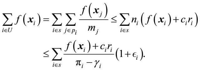
The proof is complete.

3. Variance under a General Model

It is interesting to see how well spread samples perform under a general super-population model. Following [9], but here with a possibly non-linear model, we assume

(6)

where is a Lipschitz continuous function, , , and is a Lipschitz continuous function. Moreover,

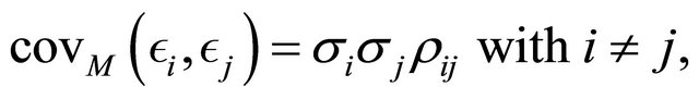
where, and are the expectation, variance and covariance under the model. The correlations are supposed to be decreasing in function of the distance between the units i and j.

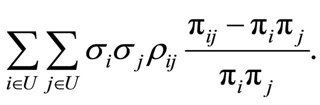
With some routine calculations, the anticipated variance of the HT-estimator under model (6) can be shown to be

(7)

where is the expectation under the design. Now, if we study expression (7), it becomes evident that we want the samples to be as balanced as possible on to minimize the term

We also want to make sure that is small whenever is large in order to minimize the term

(8)

If the samples are selected to be well spread (i.e. small joint inclusion probabilities for nearby units), then both terms in (7) becomes small. However, if the model standard deviation is known, it is possible to also choose the inclusion probabilities to minimize further. The diagonal term of (8) is dominant, i.e.

(9)

With the constraint of fixed sample size

and by using a Lagrangian function, it follows that the minimum in of the right hand side of (9) is

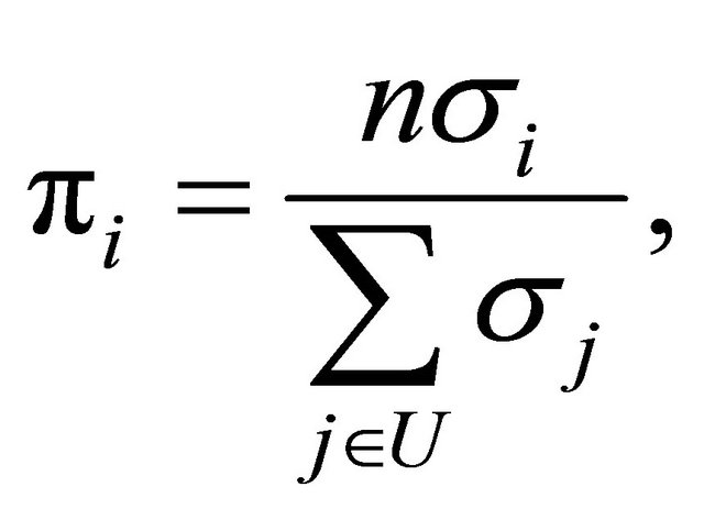(10)

if each. As a result, a very efficient sampling design under this general model is to select samples that are well spread in the x-space with inclusion probabilities given by (10). The requirements needed in order for the samples to be approximately balanced on are then fulfilled. The inclusion probabilities will not vary much within the polytopes since is supposed to be a Lipschitz continuous function of x. Hence, with this strategy, the anticipated variance of the HTestimator becomes small.

It is not possible to balance the sample directly on since the function is obviously not known in advance. Probably, the best we can do in practise is to make sure the samples are well spread in x to have a balancing effect on the unknown function, and hence also have small when may be large.

If we use well spread probability samples together with the HT-estimator, the estimator will be very efficient (i.e. have a small variance) if the population is close to a realization of the model (6). Note also that the approach is purely design based, and the estimator maintains design unbiasedness and design consistency even if the model is false.

Example 2, given in the next section, supports the above statements. In particular, the example compares different sampling methods with respect to variance and spatial balance. It is clear that methods obtaining well spread samples are more balanced and hence produce smaller variance.

4. Some Methods for Selecting Well Spread Samples

Besides spatial stratification, one of the first more novel designs for selecting a well spread sample is called generalized random tessellation stratified (GRTS), and was introduced in [2]. The GRTS design uses a specific random mapping to map two (or more) dimensions to one dimension. Basically the units are re-ordered to a list and units close in the list tend to also be close in the auxiliary space. Then a systematic ps sample is selected from the list, making sure the sample becomes well spread in the list and hence also in the auxiliary space. A drawback of GRTS is that a lot of information is lost in the mapping, especially if the space has many dimensions (i.e. many auxiliary variables). However, for two dimensions, the GRTS produces rather well spread samples.

Another idea is to map dimensions to one by use of space-filling curves, and one such design was presented and evaluated in [10]. However, we believe that mapping several dimensions to one is not the best way to achieve a well spread sample. Too much information is lost in such a mapping.

A more recent idea to achieve well spread samples is to first define a distance measure in the auxiliary space. To do so, let be all available auxiliary variables, where correspond to the quantitative variables and to the qualitative variables. To measure the distance between unit i and j in this q-dimensional space, [11] propose the following definition of distance

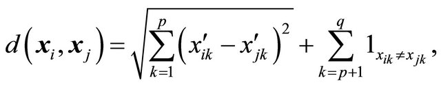
where is the standardized version of. By standardizing, the auxiliary variables are approximately of equal importance. However, the above distance function is just an example and in a particular situation some other distance function may be more appropriate. Given the distace measure, the design should create a negative correlation of the inclusion indicators for close units, so that two close units seldom appear in the sample together. Such a design is not necessarily complicated. For instance, the local pivotal method (LPM) introduced in [5] is quite simple. The LPM is based on the pivotal method [4]. The main idea in LPM is to make similar units (i.e. nearby units) compete with each other for inclusion in the sample. 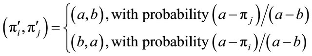The LPM successively updates the prescribed vector of inclusion probabilities to become a vector with zeros and ones, where the ones indicate inclusion in the sample. In one step of LPM, two close units i and j with and are chosen to compete. The winner takes as much probability mass as possible from the other unit. Hence, the winner receives the new probability and the looser gets the new probability. Thus, if, then a = 1 and the winning unit will definitely be in the sample. If, then the looser will definitely not be in the sample (since b = 0). The reduced probability vector is updated as

Now, replace with. The final outcome is decided for at least one unit each update, and thus the procedure has at most N steps. In each update, unit i is chosen randomly (with equal probabilities among the units with) and then its nearest neighbor (among the units with) is chosen.

Another method, spatially correlated Poisson sampling (SCPS) was first described in [6] and it is a special case of the method introduced in [7]. The SCPS algorithm is a bit more complicated than LPM, but is based on the same idea. Weights are used to create a negative correlation between the inclusion indicators of nearby units, forcing the sample to be well spread. For more on the above discussed methods, for selecting well spread samples, we refer the reader to the previously mentioned papers.

The two designs, LPM and SCPS were used in [11] to obtain well spread probability samples. The fact that LPM and SCPS produce well spread samples has been justified by both theoretical results and simulation results in the previously mentioned papers. Variance estimators for the HT-estimator under well spread samples was suggested in the papers [11,12]. To our knowledge LPM and SCPS are the designs that in general produce the lowest mean value of the balance measure (1) in general auxiliary space with prescribed inclusion probabilities.

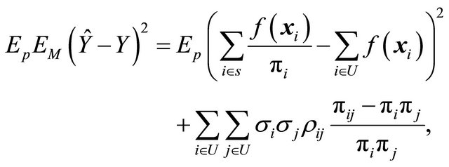
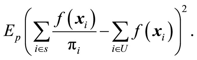
When it comes to efficiency of the HT-estimator for well spread samples, we can also make heuristic arguments that such samples produce a low variance of the HT-estimator. When the sample size is fixed, the variance of 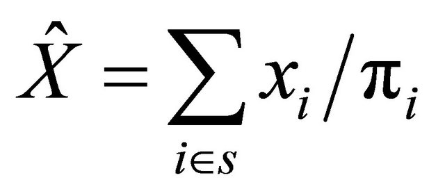can be written as

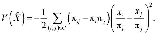(11)

A property that e.g. the LPM and SCPS design have is that is small (minimum or close to minimum) when is small and is large (close to) when

is large. If is small when is small, then is small when is smalli.e. is small when is large. Also, if is large (i.e.

is large), then is small since. As a result the variance (11) becomes small.

For well spread samples, the balancing property can only be shown to hold exactly in very specific situations, i.e. under assumptions (A.0)-(A.2), see (2). For a categorical auxiliary variable, the sample will be balanced if the design produces stratification with fixed sample size for each category. A simple example follows.

Example 1. Let U be a population of males U_m and females U_f. Let x be the only auxiliary variable and let if male and if female. Also, let and be the inclusion probabilities, where n_m and n_f are integers. In this special case, we have that e.g. the LPM and SCPS automatically produces stratification with fixed sample sizes. Hence we have

where s_m and s_f are the sampled males and females respectively.

Example 2. We compare the different sampling methods LPM, SCPS, GRTS and simple random sampling (SRS) using a model satisfying (6). In particular, the population is generated from with

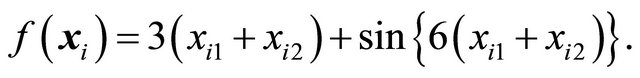
The population size is N = 200 and the x-values are generated from a uniform distribution on the unit square. Using Euclidean distance, the covariance function for is defined as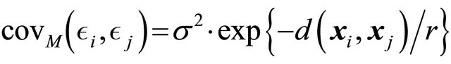, which is a simple covariance function used for stationary fields [13]. The -values are generated in two steps. First random independent and identically distributed data is generated from. Then, the -values are constructed as using the covariance matrix. In this example and. The units are sampled with equal inclusion probabilities and units are sampled.

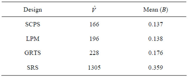
The target parameter is. In our particular realization the true value is. The result is presented in Table 1. A clear connection between well spread samples and variance can be observed. A design with a small expected value of B, see (1), gives better estimates. Concerning anticipated variance we get similar results if we average over repeated realizations from the model.

Table 1. Results for Example 2. Empirical variance of the HT-estimator and the mean of the measure B for 1000 samples of size 50.

5. Final Comments

It has been shown that in general there is a significant balancing effect for well spread samples. Usually, well spread samples are not as balanced on the auxiliary x-variables as samples selected by the cube method, but nearly so if the sample size is not too small. However, for target variables that are non-linear in x, well spread samples are likely to be more balanced on the target variables than samples selected by the cube method. In that way, well spread samples are good for more general situations. Hopefully, the fact that a significant balancing effect has been shown will increase the interest of using well spread probability samples when auxiliary x-variables are available.

There also exists a possibility to combine the cube method with a similar idea as used in the LPM, to have a local cube method. Then samples that are both well spread (spatially balanced) and balanced on the auxiliary variables can be selected. Such a method was developed in [9].

In [1,14], properties of spatial total estimators are studied under a tessellation stratified design in a continues universe. With similar assumptions on the target function, as used in this paper, they show that the convergence rate of the variance of the total estimator is for such a design. Even though our setting is different and does not imply a strict stratification, this indicates that spreading the sample locations well probably gives a small variance when there are spatial trends.

In the setting of Voronoi polytopes used in this paper, we may consider the nearest neighbor estimator (NNestimator) in place of the HT-estimator. The NN-estimator of Y is, if is the number of units in polytope,

Under the assumptions (A.0) and (A.1), we have and the NN-estimator is equal to the HT-estimator. This implies that the NN-estimator will be approximately design unbiased for well spread samples. Moreover, the NN-estimator can probably adjust for some minor spatial imbalance in the sample by using the realized polytope sizes instead of, which can be viewed as the estimated polytope sizes. The possible benefit of using the NN-estimator in place of the HTestimator will be investigated in a future paper.

6. Acknowledgements

Thanks to Lennart Bondesson and an anonymous reviewer for helpful comments that improved this manuscript.

REFERENCES

- L. Barabesi and S. Franceschi, “Sampling Properties of Spatial Total Estimators under Tessellation Stratified Designs,” Environmetrics, Vol. 22, No. 3, 2011, pp. 271- 278. doi:10.1002/env.1046
- D. L. Stevens Jr. and A. R. Olsen, “Spatially Balanced Sampling of Natural Resources,” Journal of the American Statistical Association, Vol. 99, No. 465, 2004, pp. 262- 278. doi:10.1198/016214504000000250
- J.-C. Deville and Y. Tillé, “Efficient Balanced Sampling: the Cube Method,” Biometrika, Vol. 91, No. 4, 2004, pp. 893-912. doi:10.1093/biomet/91.4.893
- J.-C. Deville and Y. Tillé, “Unequal Probability Sampling without Replacement through a Splitting Method,” Biometrika, Vol. 85, No. 1, 1998, pp. 89-101. doi:10.1093/biomet/85.1.89
- A. Grafström, N. L. P. Lundström and L. Schelin, “Spatially Balanced Sampling through the Pivotal Method,” Biometrics, Vol. 68, No. 2, 2012, pp. 514-520. doi:10.1111/j.1541-0420.2011.01699.x
- A. Grafström, “Spatially Correlated Poisson Sampling,” Journal of Statistical Planning and Inference, Vol. 142, No. 1, 2012, pp. 139-147. doi:10.1016/j.jspi.2011.07.003
- L. Bondesson and D. Thorburn, “A List Sequential Sampling Method Suitable for Real-Time Sampling,” Scandinavian Journal of Statistics, Vol. 35, No. 3, 2008, pp. 466-483. doi:10.1111/j.1467-9469.2008.00596.x
- D. G. Horvitz and D. J. Thompson, “A Generalization of Sampling without Replacement from a Finite Universe,” Journal of the American Statistical Association, Vol. 47, No. 260, 1952, pp. 663-685. doi:10.1080/01621459.1952.10483446
- A. Grafström and Y. Tillé, “Doubly Balanced Spatial Sampling with Spreading and Restitution of Auxiliary Totals,” Environmetrics, in Press, 2012. doi:10.1002/env.2194
- A. J. Lister and C. T. Scott, “Use of Space-Filling Curves to Select Sample Locations in Natural Resource Monitoring Studies,” Environmental Monitoring and Assessment, Vol. 149, No. 1-4, 2009, pp. 71-80. doi:10.1007/s10661-008-0184-y
- A. Grafström and L. Schelin, “How to Select Representative Samples,” Scandinavian Journal of Statistics, 2013.
- D. L. Stevens Jr. and A. R. Olsen, “Variance Estimation for Spatially Balanced Samples of Environmental Resources,” Environmetrics, Vol. 14, No. 6, 2003, pp. 593- 610. doi:10.1002/env.606
- N. A. C. Cressie, “Statistics for spatial data,” Wiley, New York, 1993.
- L. Barabesi and M. Marcheselli, “A Modified Monte Carlo Integration,” International Mathematical Journal, Vol. 3, No. 5, 2003, pp. 555-565.