Geomaterials
Vol.4 No.1(2014), Article ID:42124,8 pages DOI:10.4236/gm.2014.41005
Hole Cleaning Prediction in Foam Drilling Using Artificial Neural Network and Multiple Linear Regression
1Birjand University of Technology, Birjand, Iran
2School of Mining, College of Engineering, University of Tehran, Tehran, IranEmail: reza_rooki@yahoo.com
Copyright © 2014 Reza Rooki et al. This is an open access article distributed under the Creative Commons Attribution License, which permits unrestricted use, distribution, and reproduction in any medium, provided the original work is properly cited. In accordance of the Creative Commons Attribution License all Copyrights © 2014 are reserved for SCIRP and the owner of the intellectual property Reza Rooki et al. All Copyright © 2014 are guarded by law and by SCIRP as a guardian.
Received December 11, 2013; revised December 31, 2013; accepted January 7, 2014
Keywords:Foam Drilling; Hole Cleaning; Artificial Neural Network; Multiple Linear Regression
ABSTRACT
Foam drilling is increasingly used to develop low pressure reservoirs or highly depleted mature reservoirs because of minimizing the formation damage and potential hazardous drilling problems. Prediction of the cuttings concentration in the wellbore annulus as a function of operational drilling parameters such as wellbore geometry, pumping rate, drilling fluid rheology and density and maximum drilling rate is very important for optimizing these parameters. This paper describes a simple and more reliable artificial neural network (ANN) method and multiple linear regression (MLR) to predict cuttings concentration during foam drilling operation. This model is applicable for various borehole conditions using some critical parameters associated with foam velocity, foam quality, hole geometry, subsurface condition (pressure and temperature) and pipe rotation. The average absolute percent relative error (AAPE) between the experimental cuttings concentration and ANN model is less than 6%, and using MLR, AAPE is less than 9%. A comparison of the ANN and mechanistic model was done. The AAPE values for all datasets in this study were 3.2%, 8.5% and 10.3% for ANN model, MLR model and mechanistic model respectively. The results show high ability of ANN in prediction with respect to statistical methods.
1. Introduction
Underbalanced drilling (UBD) is increasingly used in the development of oil and gas fields because of minimizing the damage caused by invasion of drilling fluids into the formation, minimizing lost circulation, decreasing pressure differential sticking, increasing penetration rate, increasing production and extending bit life. UBD techniques are classified into gas, foam, gasified-liquid and liquid underbalanced drilling. The choice of drilling fluid type is determined by the formation pressure and formation properties. Foam is gaining increasing applications in the petroleum industry including drilling, cementing, fracturing and oil displacement. In drilling operations, foam can be used for both UBD and Managed Pressure Drilling (MPD). Foam fluids generally include 5% - 25% liquid phase and 75% - 95% gaseous phase. The liquid phase could be fresh water or brines. The gaseous phase is usually an inert gas. A surfactant is often used as a stabilizer and it comprises about 5% of the fluid system. The fluid system can be weighted up using heavy brines or barites. It has higher cuttings transport ability compared to air drilling fluids. Foam drilling system is recommended for many naturally fractured reservoirs where lost circulation is a main concern. With the ever increasing gas prices, foam will be an excellent candidate for drilling unconventional gas wells, for example, coal-bed methane drilling. Foam is a compressible and homogeneous mixture in comparison with the conventional and aerated drilling fluids. This makes foam a unique fluid for drilling through formations with continuously changing pressure gradients [1,2]. Hole cleaning (Cuttings transport) is one of the main factors influencing cost, time, and quality of directional, horizontal, extended reach and multilateral oil/gas wells. Inadequate hole cleaning can result in costly drilling problems such as pipe sticking, premature bit wear, slow drilling, formation fracturing and high torque and drag. Cuttings transport is mainly controlled by many variables, such as the well inclination angle, hole and drillpipe diameters, drillpipe rotation, drillpipe eccentricity, rate of penetration, cuttings characteristics (size, porosity of bed), flow rate, fluid velocity, flow regime, mud type and complex nonNewtonian mud rheology. An outstanding review of the cuttings transport discussion was given by Nazari et al. [3]. Many researchers have been carried out on cuttings transport with conventional drilling fluids in horizontal and directional wells. In addition, some empirical and mechanistic models have been developed in cuttings transport [4-6]. Foams can have extremely high viscosity, in all instances in which their viscosity is greater than that of both the liquid and the gas that they contain. At the same time, their densities are usually less than onehalf of water. They are stable at high temperatures and pressures. Hence, if foam is applied as drilling fluid, high viscosity of the foam permits efficient cuttings transport. In addition, its low density allows underbalanced conditions to be established, and formation damage to be minimized. Furthermore, compression requirement is decreased. Efficient cuttings removal is of critical significance according to multiphase flow and foam drilling hydraulic, for wells are drilled with foams [7-9]. The majority of publications of cuttings transport with foam describe operators’ experiences, field practices, 1D numerical simulation of cutting transport and equipment used [10-16]. Artificial neural networks (ANNs) are simple and more reliable predictive tools inspired by studies on the human nerve and brain system that can be used to model and investigate various highly complex and nonlinear phenomena [17-19]. ANN has been applied in the multiphase flow fields and acceptable results were achieved compared with the conventional methods incorporating correlations and mechanistic models [20-27]. The aim of this study is to determine the hole cleaning efficiency of foam fluid flow through a horizontal annuli using back propagation neural network (BPNN) from affecting parameters on cuttings transport. The BPNN model was verified by experimental data obtained from the literature. The results show that adequate accuracy was obtained by the model to predict hole cleaning efficiency.
2. Cuttings Concentration Prediction Using BPNN
The feed-forward neural networks with back propagation (BP) learning algorithm are very powerful in function optimization modelling [28,29]. BPNNs are recognised for their prediction capabilities and ability to generalise well on a wide variety of problems. Automated Bayesian Regularization (ABR) method can be applied to avoid over fitting problem in BPNN [27]. In this study, 77 cutting transport experimental datasets at Tulsa University obtained from the literature [8,9] were used to create BPNN model. Table 1 gives test matrix of experiments. Input parameters of BPNN include foam velocity (V), foam quality ( ), eccentricity of annulus(
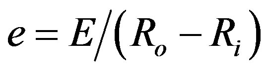 )where E is offset distance between the centers of the inner tube, Ri, and the outer tube, Ro, of annulus), subsurface condition (pressure, P, and temperature, T), and pipe rotation (RPM). Other parameters in Table 1 are constant. The output of network is cutting concentration (CC%) in annulus.
Table 2 outlines the correlation matrix between cuttings concentration (CC) and independent variables that effect on cuttings transport using SPSS software. According to this table, foam quality ( ), foam velocity (V) and pipe rotation (RPM) are more effective on cuttings transport phenomenon.
Considering the requirements of the ANN computation algorithm (better identification of parameters), both input and output data were normalised to an interval by a simple transformation process. In this study, normalization of data was carried out within the range of  using Equation (1) [17],
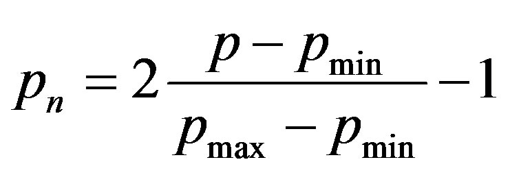 (1)
(1)
where, pn is the normalised parameter, p denotes the actual parameter, pmin represents a minimum of the actual parameters and pmax stands for a maximum of the actual parameters. About 70% of the total data sets (60 out of 77 of the data) were selected for training and the rest for testing purposes. Several architectures comprising varied numbers of neurons in hidden layer with ABR algorithm were tried to predict cutting concentration using BPNN.
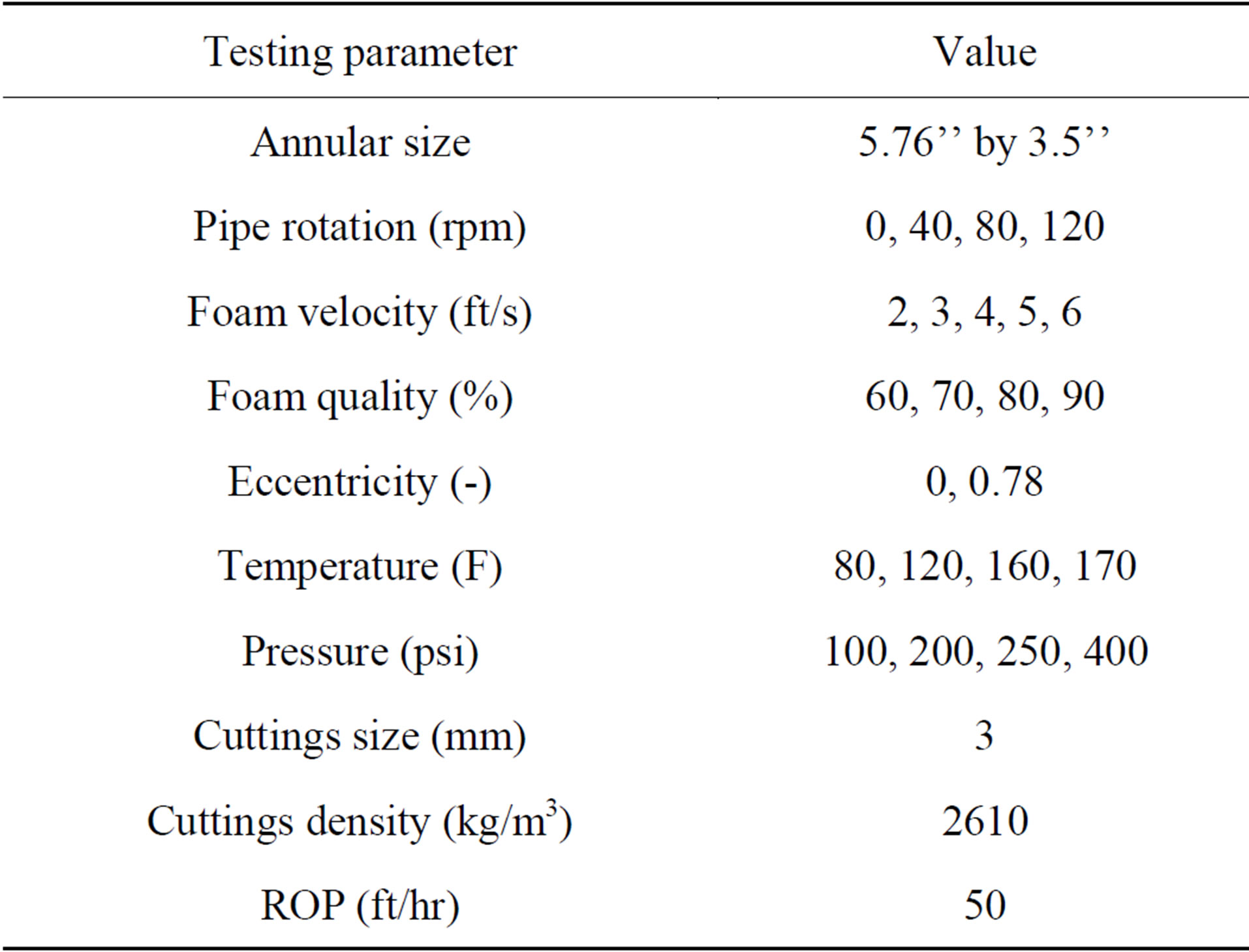
Table 1. Test matrix of cuttings transport using aqueous foam [8,9].
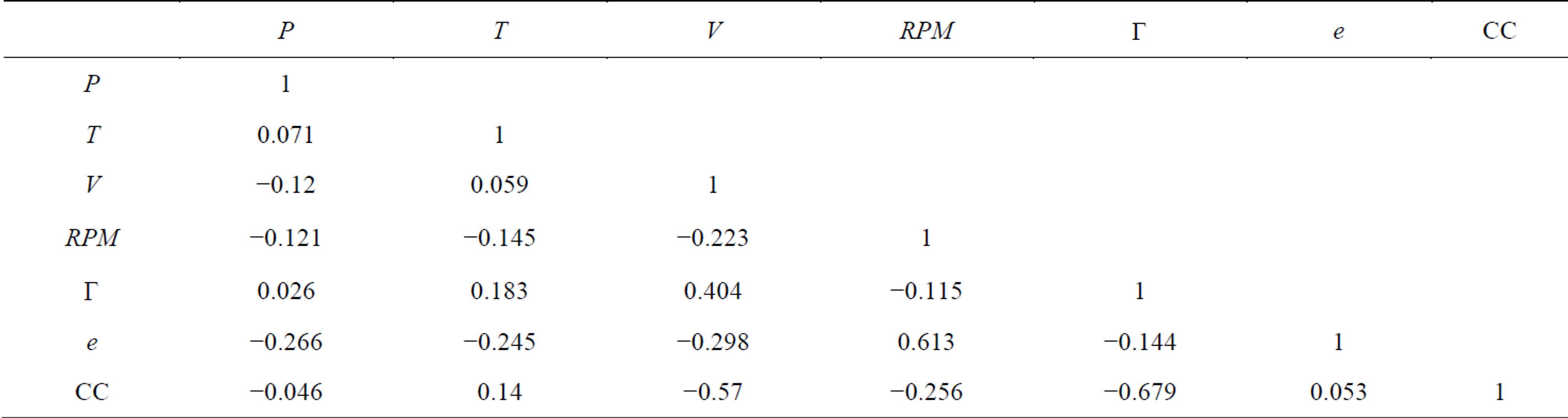
Table 2. Correlation matrix between cuttings concentration and independent variables.
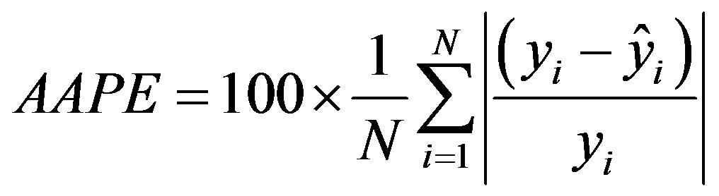
Two criteria were employed in order to assess the effectiveness of each network and its ability to make accurate predictions; they are: average absolute percent relative error (AAPE) and the correlation coefficient (R) [31].
The AAPE concept gives an idea of absolute relative deviation of estimated from the measured data. It can be calculated from the following equation:
 (2)
(2)
where,  is the measured value,
  denotes the predicted value, and N stands for the number of samples. The lowest AAPE values, the more accurate the prediction is.
The last measure, known as the efficiency criterion, R represents the percentage of the initial uncertainty explained by the model. It is given by:
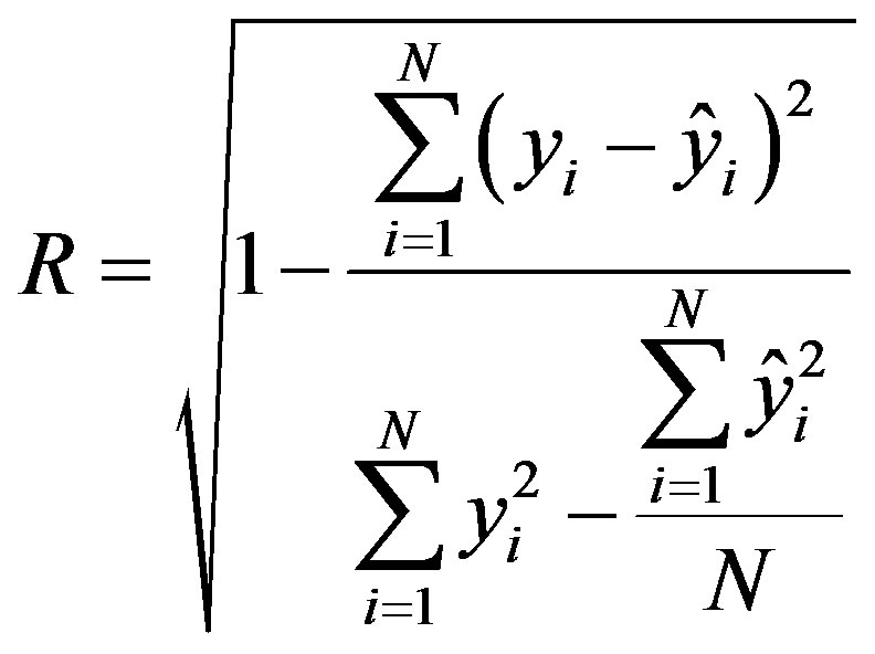 (3)
(3)
The best fitting between predicted and measured values, which is unlikely to occur, would have RMS = 0 or R = 1. The optimal network of this study is a feed forward multilayer perceptron [28,29]. This network comprises one input layer with 6 inputs (P, T, V, RPM, e, ) and one hidden layer with 10 neurons. Fletcher and Goss [30] suggested that the appropriate number of nodes in a hidden layer varies between (
 + m) and (2n + 1), where n is the number of input nodes and m represents the number of output nodes. Each neuron has a bias and is fully connected to all inputs and employs a log-sigmoid activation function. The output layer has one neuron (CC%) with a linear activation function (purelin) without bias. Training function of this network is ABR algorithm (trainbr). In this study, (n = 6) and (m = 1) and thus the appropriate number of hidden layer neurons was chosen as 10 (6-10-1). Figure 1 shows the BPNN architecture constructed in this work.
3. Cuttings Concentration Prediction Using MLR
Multiple linear regression (MLR) is an extension of the regression analysis that incorporates additional independent variables in the predictive equation. Here, the model to be fitted is:
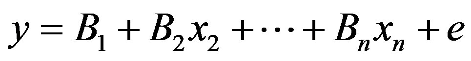 (4)
(4)
where, y is the dependent variable, xis are the independent random variables and e is a random error (or residual) which is the amount of variation in y not accounted for by the linear relationship. The parameters Bis, stand for the regression coefficients, are unknown and are to be estimated. However, there is usually substantial variation of the observed points around the fitted regression line. The deviation of a particular point from the regression line (its predicted value) is called the residual value. The smaller the variability of the residual values around the regression line, the better is model prediction. In this study, regression analysis was performed using the train and test data employed in neural network data. The cuttings concentration considered as the dependent variable and V,  , P, T, RPM and e were considered as the independent variables. A computer-based package called SPSS (Statistical Package for the Social Sciences) was used to carry out the regression analysis.
4. Results and Discussion
4.1. BPNN Results
Using the BPNN approach described above, all necessary computations were implemented by supplying extra codes in MATLAB software. The matrix of inputs in training step is a n × N vector, where n is the number of network inputs and N is the number of samples used in training step. In this paper, six input variables (V,  , P, T, RPM, e) and 60 samples were used to train the network; therefore n × N = 6 × 60. The matrix of outputs in training step, is a m × N vector, where m is the number of outputs. In this study, there is only one output so, m × N = 1 × 60. In the same manner, the matrices of inputs and
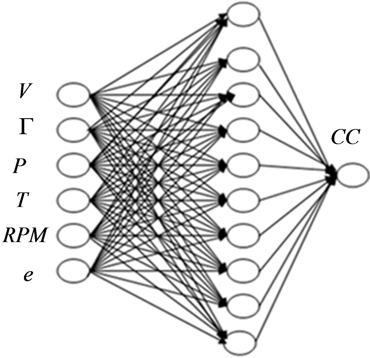
Figure 1. BPNN architecture (6-10-1).
output for testing phase, were n × N = 6 × 17 and m × N = 1 × 17 respectively. The correlation coefficient (R) and AAPE were used for comparison of the ANN model predictions with experimental data [8,9] and the results of mechanistic model [9,16]. Figure 2 compares the predicted cuttings volumetric concentration (%) and the experimental values for the training data set. The correlation coefficient (R) to the linear fit (y = ax) is 0.993 with the AAPE value of 2.38%; describing almost a perfect fit. This indicates the fact that the training stage was done very well.
For testing stage, those data sets which were not employed by the ANN model during training process were used. A comparison of the cutting concentrations predicted by the network and the measured values for the test data set is shown in Figure 3. A correlation coefficient (R) of 0.914 together with an AAPE of 5.93% describes a very satisfactory model performance. These results verified the success of neural networks which recognize the implicit relationships between input and output variables.
A comparison of the network predictions and the measured values for the all data sets used in this study with a population of 77 is shown in Figure 4. The correlation coefficient (R) is 0.984 with an AAPE of 3.18%; indicating a very satisfactory model performance. These results verified the success of neural networks which recognise the implicit relationships between input and output variables.
4.2. MLR Results
Using MLR approach in SPSS software, the estimated regression relationship for cuttings concentration (CC) is given as below:
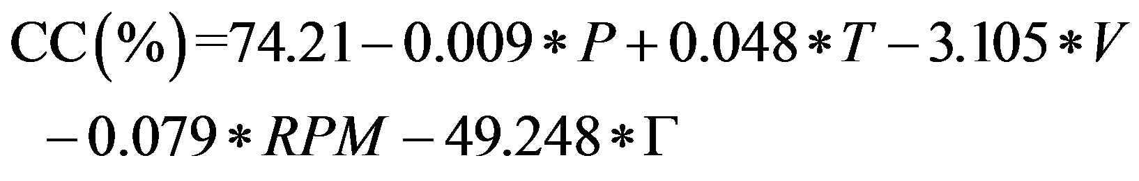 (5)
(5)
The statistical results of the model are given in Table 3.
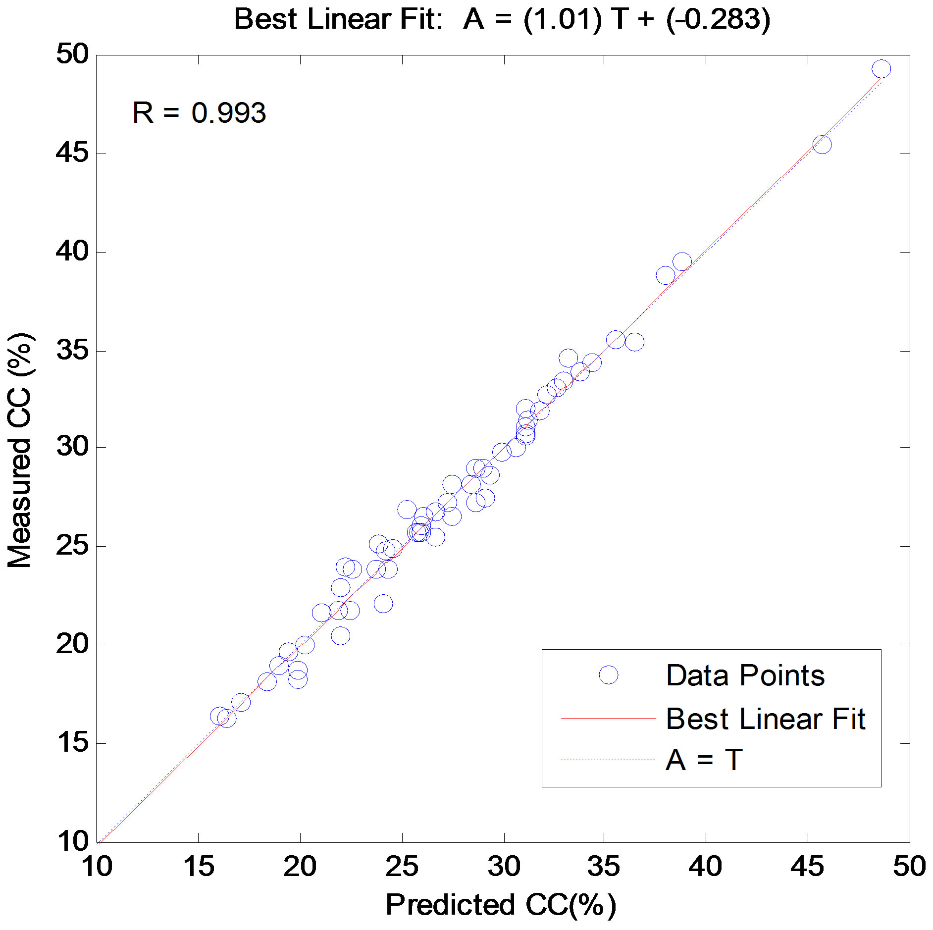
Figure 2. ANN prediction versus measured cutting concentration [8,9] for the training data.
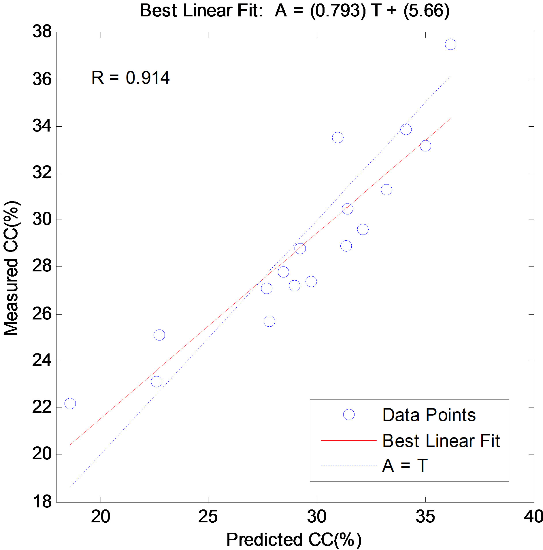
Figure 3. ANN prediction versus measured cutting concentration [8,9] for the test data.
Cuttings concentration was estimated according to the Equations 5. Figures 5 and 6 compare the MLR cuttings concentration (%) versus the experimental values for the training and test data set respectively. The correlation coefficient (R) and AAPE for train data are 0.916 and 6.5% and for test data, they are 0.84 and 7%.
A comparison of the ANN, MLR and mechanistic model [9,16] predictions with the measured values for the all data sets used in this study with a population of 77 is shown in Figure 7. The correlation coefficient (R) is
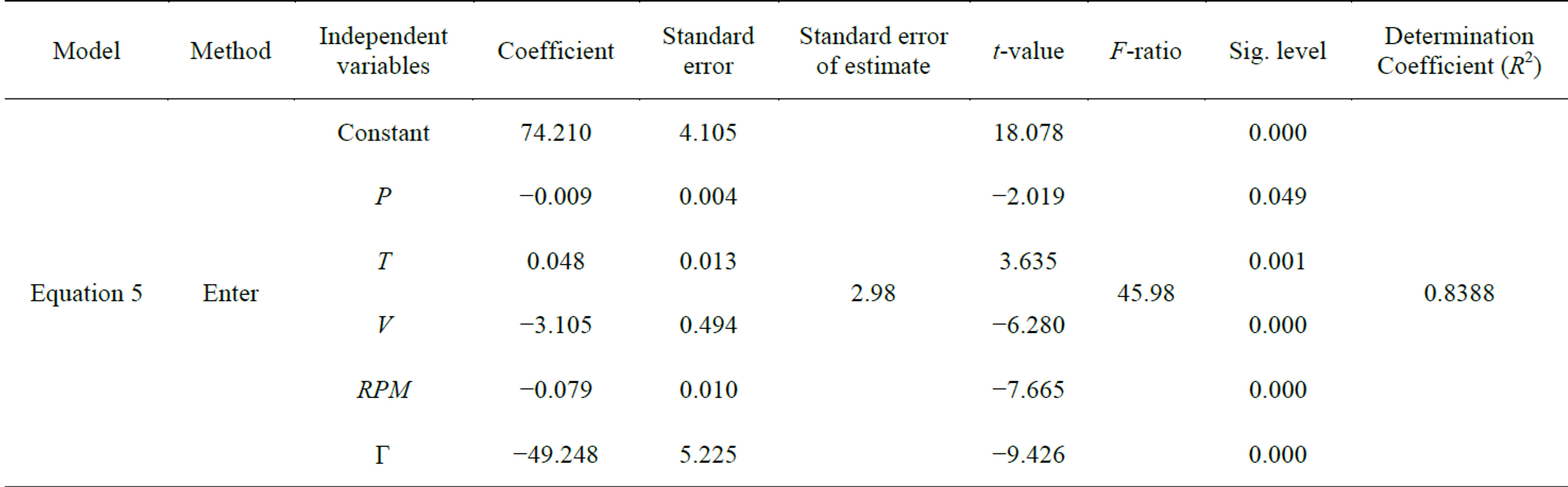
Table 3. Statistical characteristics of the multiple regression models.
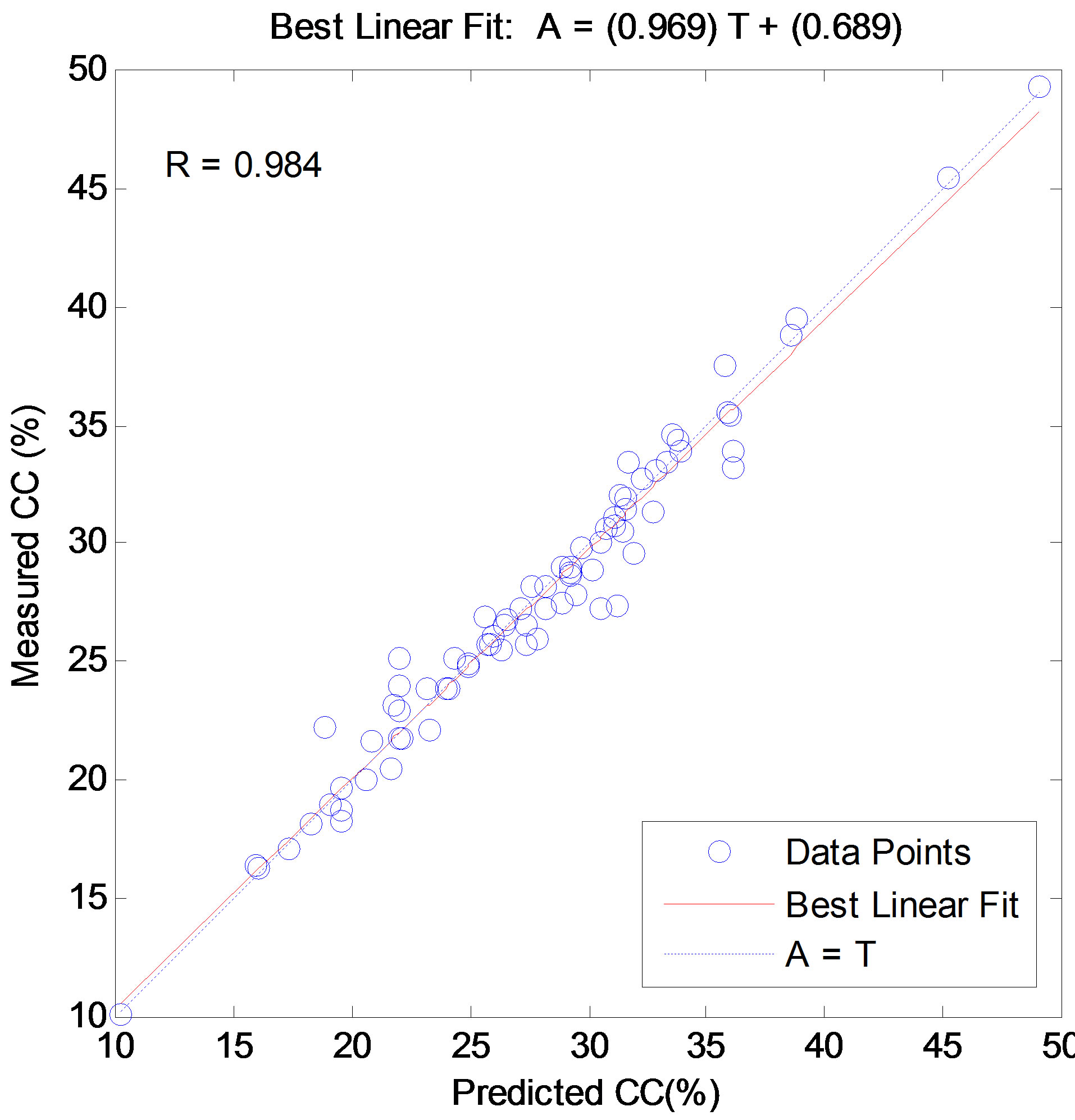
Figure 4. ANN prediction versus measured cutting concentration (%) for the all data [8,9].
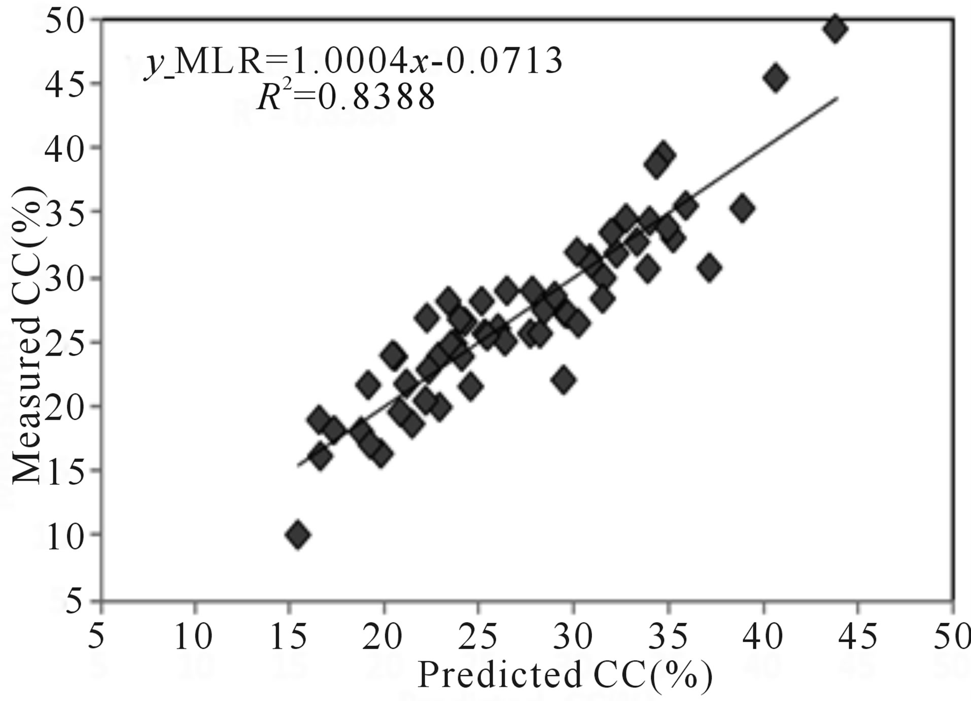
Figure 5. MLR prediction versus measured cutting concentration [8,9] for the train data.
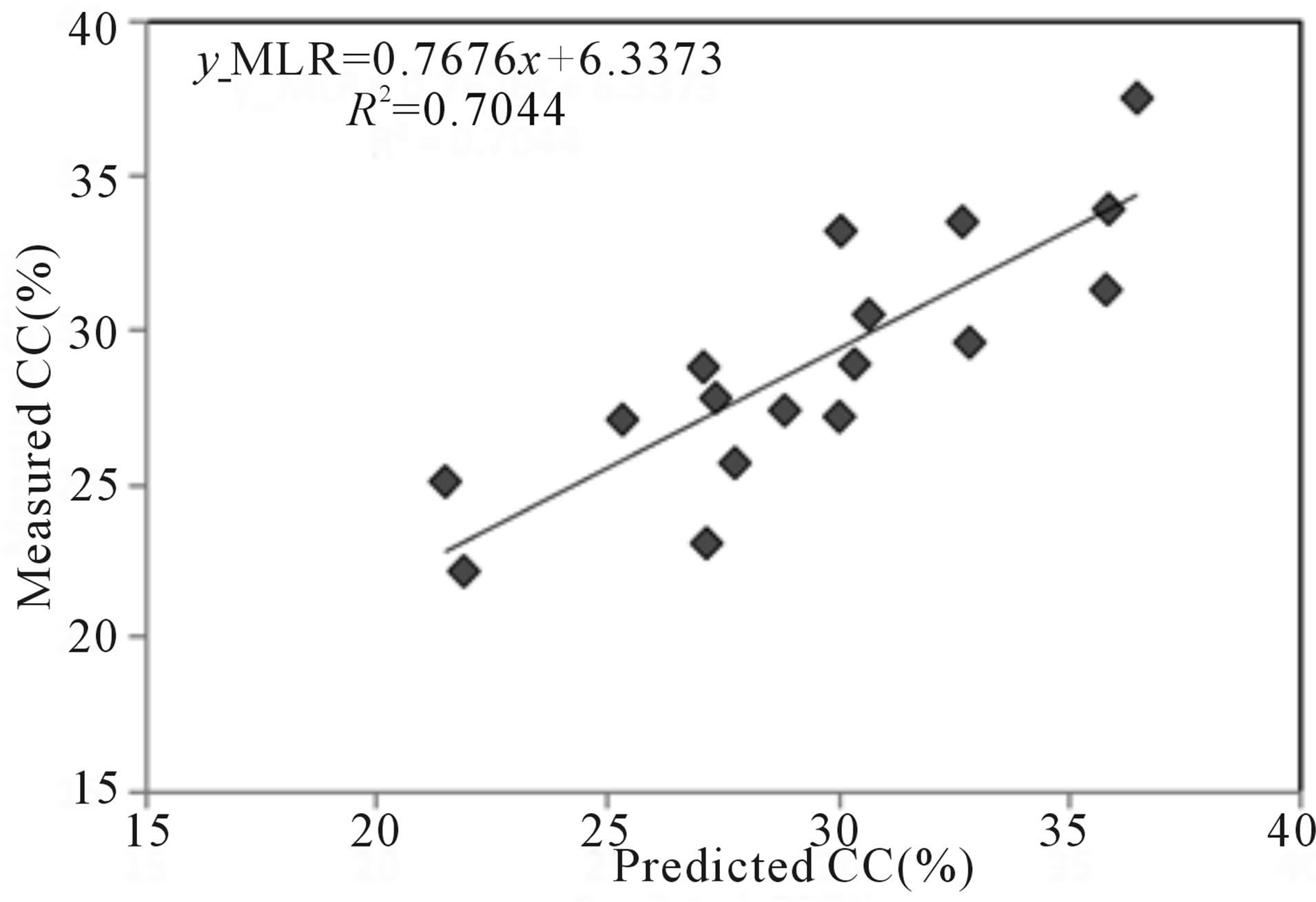
Figure 6. MLR prediction versus measured cutting concentration [8,9] for the test data.
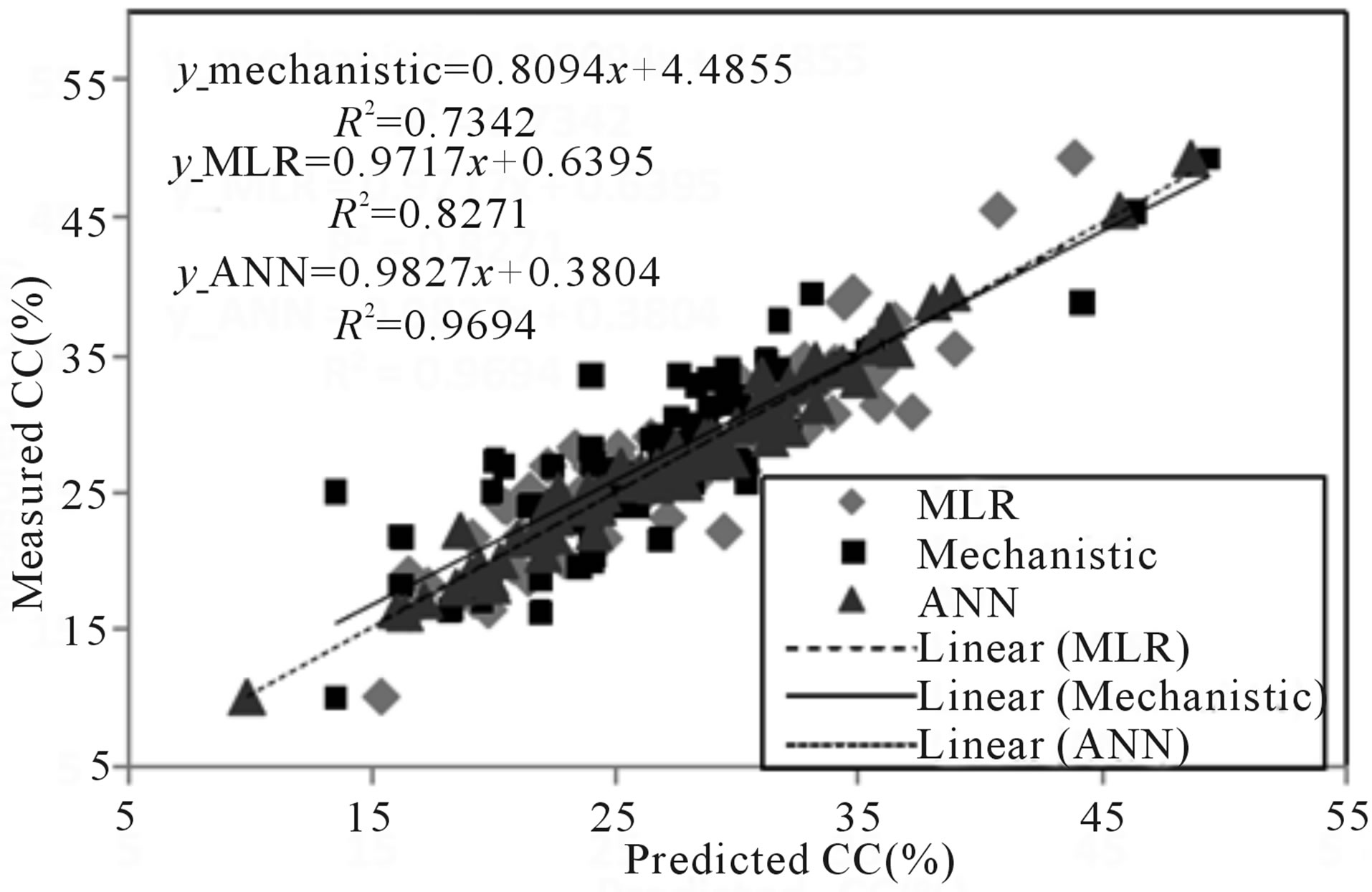
Figure 7. Comparison of measured all datasets versus ANN, MLR and mechanistic model predictions.
0.984, 0.909 and 0.8568 for ANN, MLR and mechanistic model respectively. The AAPE values are 3.2%, 8.5% and 10.3% for ANN, MLR and mechanistic model respectively.
Table 4 compares the results of ANN, MLR and mechanistic models for measured data from Duan [9] and from Chen [8]. It is well illustrated in Table 4 that the
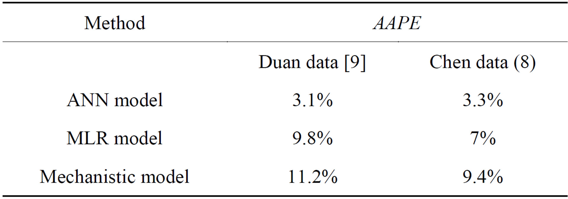
Table 4. The comparison of the results of three methods.
ANN method has high capability in prediction respect to statistical and mechanistic models.
5. Conclusion
In this study, cuttings concentration within the foam drilling in horizontal annular geometries was estimated using ANN and MLR models. The ANN presented here has three layers, namely, input layer, hidden layer and output layer. Input layer has six neurons including foam velocity, foam quality, eccentricity of annulus, subsurface condition (pressure and temperature) and pipe rotation. Hidden layer has ten neurons with a log-sigmoid activation function in all neurons. Output layer has one neuron (cutting concentration, CC%) with a purelin activation function. The correlation coefficients between measured and prediction values in training and testing data are 0.994 and 0.914 respectively. The AAPE values of training and testing data in ANN model are 2.38% and 5.93% respectively. A comparison of the ANN, MLR and mechanistic model was done. The results obtained from this study reveal that ANN could accurately predict the hole cleaning efficiency using foam drilling with respect to MLR and mechanistic models.
REFERENCES
- T. Zhu, L. Volk and H. Carroll, “Industry State-of-the-Art in Underbalanced Drilling,” Project Report, 1995.
- R. Wang, R. Cheng, H. Wang and Y. Bu, “Numerical Simulation of Transient Cuttings Transport with Foam Fluid in Horizontal Wellbore,” Journal of Hydrodynamics, Vol. 21, No. 4, 2009, pp. 437-444. http://dx.doi.org/10.1016/S1001-6058(08)60169-9
- T. Nazari, G. Hareland and J. J. Azar, “Reviw of Cuttings Transport in Directional Well Drilling, Systematic Approach,” SPE 132372, California, 2010.
- T. I. Larsen, A. A. Pilehvari and J. J. Azar, “Development of a New Cutting Transport Model for High Angle Wellbores Including Horizontal Wells,” SPE Drilling and Completion, Vol. 12, No. 2, 1997, pp. 129-136. http://dx.doi.org/10.2118/25872-PA
- M. Yu, N. E. Takach, D. R. Nakamura and M. M. Shariff, “An Experimental Study of hole Cleaning under Simulated Downhole Conditions,” Saudi Aramco of Technology, 2007, pp. 2-16.
- B. V. Loureiro, R. S. de Paula and M. B. Serafim, “Experimental Evaluation of the Effect of Drillstring Rotation in the Suspension of a Cuttings Bed,” SPE Latin American and Caribbean Petroleum Engineering Conference, Lima, 1-3 December 2010, 14 p. http://dx.doi.org/10.2118/122071-MS
- M. E. Ozbayoglu, S. Z. Miska, T. Reed and N. Takach, “Using foam in Horizontal Well Drilling, a Cuttings Transport Modeling Approach,” Journal of Petroleum Science and Engineering, Vol. 46, No. 4, 2005, pp. 267- 282. http://dx.doi.org/10.1016/j.petrol.2005.01.006
- Z. Chen, “Cuttings Transport with Foam in Horizontal Concentric Annulus under Elevated Pressure and Temperature Conditions,” Ph.D. Thesis, Tulsa University, Tulsa, 2005.
- M. Duan, “Study of Cuttings Transport Using Foam with Drill Pipe Rotation under Simulated Downhole Conditions,” Ph.D. Thesis, Tulsa University, Tulsa, 2007.
- S. Saintpere, Y. Marcillat, F. Bruni and A. Toure, “Hole Cleaning Capabilities of Drilling Foams Compared to Conventional Fluids,” SPE Annual Technical Conference and Exhibition, Texas, 2000.
- A. L. Martins, A. M. F. Luorenco and C. H. M. de Sa, “Foam Properties Requirements for Proper Hole Cleaning While Drilling Horizontal Wells in Underbalanced Conditions,” SPE Drilling and Completion, Vol. 16, No. 4, 2001, pp.195-200. http://dx.doi.org/10.2118/74333-PA
- Y. Li and E. Kuru, “Numerical Modeling of Cuttings Transport with Foam in Horizontal Wells,” Journal of Canadian Petroleum Technology, Vol. 42, No. 10, 2003, pp. 54-61. http://dx.doi.org/10.2118/03-10-06
- Y. Li and E. Kuru, “Numerical Modeling of Cuttings Transport with Foam in Vertical Wells,” Journal of Canadian Petroleum Technology, Vol. 44, No. 3, 2005, pp. 31-39.
- J. Capo, M. Yu, S. Z. Miska, N. E. Takach and R. Ahmed, “Cuttings Transport with Aqueous foam at Intermediate Inclined Wells,” SPE Drilling and Completion, Vol. 21, No. 2, 2006, pp. 99-107. http://dx.doi.org/10.2118/89534-PA
- Z. Chen, R. M. Ahmed, S. Z. Miska, N. E. Takach, M. Yu, M. B. Pickell and J. Hallman, “Experimental study on cuttings transport with foam under simulated horizontal downhole conditions,” SPE Drilling and Completion, Vol. 22, No. 4, 2007, pp. 304-312. http://dx.doi.org/10.2118/99201-PA
- M. Duan, S. Miska, M. Yu, N. Takach, R. Ahmed and J. Hallma, “Experimental Study and Modeling of Cuttings Transport Using Foam with Drillpipe Rotation,” SPE Drilling and Completion, Vol. 25, No. 3, 2010, pp. 352- 362. http://dx.doi.org/10.2118/116300-PA
- H. Demuth and M. Beale, “Neural Network Toolbox for Use with MATLAB,” Handbook, 2002.
- S. Haykin, “Neural Networks: A Comprehensive Foundation,” 2nd Edition, Prentice Hall, Upper Saddle River, 1999.
- M. T. Hagan, H. B. Demuth and M. H. Beale, “Neural network design,” PWS Publishing, Boston, 1996.
- J. Ternyik, H. I. Bilgesu and S. Mohaghegh, “Virtual Measurements in Pipes: Part 2, Liquid Holdup and Flow Pattern Correlations,” SPE Eastern Regional Conference & Exhibition, Morgantown, 18-20 September 1995, 5 p.
- M. E. Ozbayoglu, S. Z. Miska, T. Reed and N. Takach, “Analysis of Bed Height in Horizontal and Highly-Inclined Wellbores by Using Artificial Neural Networks,” International Horizontal Well Technology Conference, Calgary, 4-7 November 2002, 7 p.
- E. S. A. Osman, “Artificial Neural Network Models for Identifying Flow Regimes and Predicting Liquid Holdup in Horizontal Multiphase Flow,” SPE Production & Facilities, Vol. 19, No. 1, 2004, pp. 33-40. http://dx.doi.org/10.2118/86910-PA
- M. E. Shippen and S. L. Scott, “A Neural Network Model for Prediction of Liquid Holdup in Two-Phase Horizontal Flow,” SPE Production & Facilities, Vol. 19, No. 2, 2004, pp. 67-76. http://dx.doi.org/10.2118/87682-PA
- E. M. Ozbayoglu and M. A. Ozbayogl, “Estimating Flow Patterns and Frictional Pressure Losses of Two-Phase Fluids in Horizontal Wellbores Using Artificial Neural Networks,” Petroleum Science and Technology, Vol. 27, No. 2, 2009, pp. 135-149. http://dx.doi.org/10.1080/10916460701700203
- R. Ashena and J. Moghadasi, “Bottom Hole Pressure Estimation Using Evolved Neural Networks by Real Coded Ant Colony Optimization and Genetic Algorithm,” Journal of Petroleum Science and Engineering, Vol. 77, No. 3-4, 2011, pp. 375-385. http://dx.doi.org/10.1016/j.petrol.2011.04.015
- A. E. F. Monfared, M. Ranjbar, H. Nezamabadi Pour, M. Schaffie and R. Ashena, “Substantial Improvement of the Bottom Hole Circulating Pressure Prediction by the Combination of GA and ANFIS,” Energy Source Part A, Vol. 33, No. 24, pp. 2272-2280.
- R. Rooki, F. Doulati Ardejani, A. Moradzadeh, V. C. Kelessidis and M. Nourozi, “Prediction of Terminal Velocity of Solid Spheres Falling through Newtonian and Non-Newtonian Power Law Pseudoplastic Fluid Using Artificial Neural Network,” International Journal of Mineral Processing, Vol. 110-111, 2012, pp. 53-61. http://dx.doi.org/10.1016/j.minpro.2012.03.012
- G. Cybenko, “Approximation by Superposition of a Sigmoidal Function,” Mathematics of Control, Signals and Systems, Vol. 2, No. 4, 1989, pp. 303-314. http://dx.doi.org/10.1007/BF02551274
- K. Hornik, M. Stinchcombe and H. White, “Multilayer Feed Forward Networks Are Universal Approximates,” Neural Networks, Vol. 2, No. 5, 1989, pp. 359-366. http://dx.doi.org/10.1016/0893-6080(89)90020-8
- D. Fletcher and E. Goss, “Forecasting with Neural Networks: An Application Using Bankruptcy Data,” Inform Manage, Vol. 24, No. 3, 1993, pp. 159-167.
- SPSS Inc., “PASW® Statistics 18 Core System User’s Guide,” 233 South Wacker Drive, 11th Floor Chicago, IL60606-6412, 1993.
Nomenclature
AAN: Artificial neural network AAPE: Average absolute percent relative error (%)
BPNN: Back Propagation neural network E: Offset distance between the centers of the inner tube and outer tube e: Eccentricity of annulus (-)
MLR: Multiple linear regression P: Pressure (psi)
R: Correlation coefficient (-)
Ri: tube radius (in)
ROP: Rate of penetration (ft/hr)
RPM: Pipe rotation (rpm)
T: Temperature ( )
)
V: Foam velocity (ft/s)
Greek Letters
 : Foam quality (%)
SI Metric Conversion Factors
ft × 0.3048 E + 00 = m in × 25.4 E − 03 = m psi 6.8948 E − 03 = MPa