American Journal of Computational Mathematics
Vol.4 No.2(2014), Article ID:44144,11 pages DOI:10.4236/ajcm.2014.42009
Derivative of a Determinant with Respect to an Eigenvalue in the Modified Cholesky Decomposition of a Symmetric Matrix, with Applications to Nonlinear Analysis
Mitsuhiro Kashiwagi
School of Industrial Engineering, Tokai University, Kumamoto, Japan
Email: mkashi@tokai-u.jp
Copyright © 2014 by author and Scientific Research Publishing Inc.
This work is licensed under the Creative Commons Attribution International License (CC BY).
http://creativecommons.org/licenses/by/4.0/


Received 8 November 2013; revised 8 December 2013; accepted 15 December 2013
ABSTRACT
In this paper, we obtain a formula for the derivative of a determinant with respect to an eigenvalue in the modified Cholesky decomposition of a symmetric matrix, a characteristic example of a direct solution method in computational linear algebra. We apply our proposed formula to a technique used in nonlinear finite-element methods and discuss methods for determining singular points, such as bifurcation points and limit points. In our proposed method, the increment in arc length (or other relevant quantities) may be determined automatically, allowing a reduction in the number of basic parameters. The method is particularly effective for banded matrices, which allow a significant reduction in memory requirements as compared to dense matrices. We discuss the theoretical foundations of our proposed method, present algorithms and programs that implement it, and conduct numerical experiments to investigate its effectiveness.
Keywords:Derivative of a Determinant with Respect to an Eigenvalue; Modified Cholesky Decomposition; Symmetric Matrix; Nonlinear Finite-Element Methods; Singular Points

1. Introduction
The increasing complexity of computational mechanics has created a need to go beyond linear analysis into the realm of nonlinear problems. Nonlinear finite-element methods commonly employ incremental techniques involving local linearization, with examples including load-increment methods, displacement-increment methods, and arc-length methods. Arc-length methods, which seek to eliminate the drawbacks of load-increment methods by choosing an optimal arc-length, are effective at identifying equilibrium paths including singular points.
In previous work [1] , we proposed a formula for the derivative of a determinant with respect to an eigenvalue, based on the trace theorem and the expression for the inverse of the coefficient matrix arising in the conjugate-gradient method. In subsequent work [2] -[4] , we demonstrated that this formula is particularly effective when applied to methods of eigenvalue analysis. However, the formula as proposed in these works was intended for use with iterative linear-algebra methods, such as the conjugate-gradient method, and could not be applied to direct methods such as the modified Cholesky decomposition. This limitation was addressed in Reference [5] , in which, by considering the equations that arise in the conjugate-gradient method, we applied our technique to the LDU decomposition of a nonsymmetric matrix (a characteristic example of a direct solution method) and presented algorithms for differentiating determinants of both dense and banded matrices with respect to eigenvalues.
In the present paper, we propose a formula for the derivative of a determinant with respect to an eigenvalue in the modified Cholesky decomposition of a symmetric matrix. In addition, we apply our formula to the arc-length method (a characteristic example of a solution method for nonlinear finite-element methods) and discuss methods for determining singular points, such as bifurcation points and limit points. When the sign of the derivative of the determinant changes, we may use techniques such as the bisection method to narrow the interval within which the sign changes and thus pinpoint singular values. In addition, solutions obtained via the Newton-Raphson method vary with the derivative of the determinant, and this allows our proposed formula to be used to set the increment. The fact that the increment in the arc length (or other quantities) may thus be determined automatically allows us to reduce the number of basic parameters exerting a significant impact on a nonlinear finite-element method. Our proposed method is applicable to the  decomposition of dense matrices, as well as to the
  decomposition of banded matrices, which afford a significant reduction in memory requirements compared to dense matrices. In what follows, we first discuss the theoretical foundations of our proposed method and present algorithms and programs that implement it. Then, we assess the effectiveness of our proposed method by applying it to a series of numerical experiments on a three-dimensional truss structure.
2. Derivative of a Determinant with Respect to an Eigenvalue in the Modified Cholesky Decomposition
The derivation presented in this section proceeds in analogy to that discussed in Reference 5. The eigenvalue problem may be expressed as follows. If ![]() is a real-valued symmetric
is a real-valued symmetric  matrix (specifically, the tangent stiffness matrix of a finite-element analysis), then the standard eigenvalue problem takes the form
 , (1)
, (1)
where  and
and  denote the eigenvalue and eigenvector, respectively. In order for equation (1) to have trivial solutions, the matrix
  must be singular, i.e.,
 . (2)
. (2)
We will use the notation  for the left-hand side of this equation:
 . (3)
. (3)
Applying the trace theorem, we find
 , (4)
, (4)
where
 . (5)
. (5)
In the case of  decomposition, we have
 (6)
(6)
with factors L and D of the form
 , (7)
, (7)
 . (8)
. (8)
The matrix  has the form
 . (9)
. (9)
Expanding the relation  (where
 ![]() is the identity matrix) and collecting terms, we find
is the identity matrix) and collecting terms, we find
![]() . (10)
. (10)
Equation (10) indicates that  must be computed for all matrix elements; however, for matrix elements outside the bandwidth, we have
 , and thus the computation requires only elements
  within the bandwidth. This implies that a narrower bandwidth gives a greater reduction in computation time.
From equation (4), we see that evaluating the derivative of a determinant requires only the diagonal elements of the inverse matrix (6). Upon expanding the product  using equations (7-9) and summing the diagonal elements, equation (4) takes the form
 . (11)
This equation demonstrates that the derivative of the determinant may be computed from the elements of the inverses of the matrices D and L obtained from the modified Cholesky decomposition. As noted above, only matrix elements within the a certain bandwidth of the diagonal are needed for this computation, and thus computations even for dense matrices may be carried out as if the matrices were banded. Because of this, we expect dense matrices not to require significantly more computation time than banded matrices.
By augmenting an  decomposition program with an additional routine (which simply adds one additional vector), we easily obtain a program for evaluating the quantity
 . The value of this quantity may be put to effective use in Newton-Raphson approaches to the numerical analysis of bifurcation points and limit points in problems such as large-deflection elastoplastic finite-element analysis. Our proposed method is easily implemented as a minor additional step in the process of solving simultaneous linear equations.
3. Algorithms Implementing the Proposed Method
3.1. Algorithm for Dense Matrices
We first present an algorithm for dense matrices. The arrays and variables appearing in this algorithm are as follows.
1) Computation of the modified Cholesky decomposition of a matrix together with its derivative with respect to an eigenvalue
(1) Input data A : given symmetric coefficient matrix,2-dimension array as A(n,n)
b : work vector, 1-dimension array as b(n)
n : given order of matrix A and vector b eps : parameter to check singularity of the matrix output
(2) Output data A : L matrix and D matrix, 2-dimension array as A(n,n)
fd : differentiation of determinant
ichg : numbers of minus element of diagonal matrix D (numbers of eigenvalue)
ierr : error code
=0, for normal execution
=1, for singularity
(3) LDLT decomposition
ichg=0
do i=1,n
do k=1,i-1
A(i,i)=A(i,i)-A(k,k)*A(i,k)2
end do
if (A(i,i)<0) ichg=ichg+1
if (abs(A(i,i)) ierr=1 return end if do j=i+1,n do k=1,i-1 A(j,i)=A(j,i)-A(j,k)*A(k,k)*A(i,k) end do A(j,i)=A(j,i)/A(i,i) end do end do ierr=0 (4) Derivative of a determinant with respect to an eigenvalue (fd) fd=0 do i=1,n <(i,i). fd=fd-1/A(i,i) <(i,j)> do j=i+1,n b(j)=-A(j,i) do k=1,j-i-1 b(j)=b(j)-A(j,i+k)*b(i+k) end do fd=fd-b(j)2/A(j,j) end do end do 2) Calculation of the solution (1) Input data A : L matrix and D matrix, 2-dimension array as A(n,n) b : given right hand side vector, 1-dimension array as b(n) n : given order of matrix A and vector b (2) Output data b : work and solution vector, 1-dimension array (3) Forward substitution do i=1,n do j=i+1,n b(j)=b(j)-A(j,i)*b(i) end do end do (4) Backward substitution do i=1,n b(i)=b(i)/A(i,i) end do do i=1,n ii=n-i+1 do j=1,ii-1 b(j)=b(j)-A(ii,j)*b(ii) end do end do 3.2. Algorithm for Banded Matrices We next present an algorithm for banded matrices. The banded matrices considered here are depicted schematically in Figure 1. In what follows, 1) Computation of the modified Cholesky decomposition of a matrix together with its derivative with respect to an eigenvalue (1) Input data A : given coefficient band matrix, 2-dimension array as A(n,nq) b : work vector, 1-dimension array as b(n) n : given order of matrix A nq : given half band width of matrix A eps : parameter to check singularity of the matrix (2) Output data A : L matrix and D matrix, 2-dimension array fd : differential of determinant ichg : numbers of minus element of diagonal matrix D (numbers of eigenvalue) ierr : error code =0, for normal execution =1, for singularity (3) LDLT decomposition ichg=0 do i=1,n do j=max(1,i-nq+1),i-1 A(i,nq)=A(i,nq) -A(j,nq)*A(i,nq+j-i)2 end do if (A(i,nq)<0) ichg=ichg+1 if (abs(A(i,nq)) ierr=1 return end if do j=i+1,min(i+nq-1,n) aa=A(j,nq+i-j) do k=max(1,j-nq+1),i-1 aa=aaA(i,nq+k-i)*A(k,nq)*A(j,nq+k-j) end do A(j,nq+i-j)=aa/A(i,nq) end do end do ierr=0 (4) Derivative of a determinant with respect to an eigenvalue (fd) fd=0 do i=1,n <(i,i)> fd=fd-1/A(i,nq) <(i,j)> do j=i+1,min(i+nq-1,n) b(j)=-A(j,nq-(j-i)) do k=1,j-i-1 b(j)=b(j)-A(j,nq-(j-i)+k)*b(i+k) end do fd=fd-b(j)2/A(j,nq) end do do j=i+nq,n b(j)=0 do k=1,nq-1 b(j)=b(j)-A(j,k)*b(j-nq+k) end do fd=fd-b(j)2/A(j,nq) end do end do 2) Calculation of the solution (1) Input data A : given decomposed coefficient band matrix,2-dimension array as A(n,nq) b : given right hand side vector, 1-dimension array as b(n) n : given order of matrix A and vector b nq : given half band width of matrix A (2) Output data b : solution vector, 1-dimension array (3) Forward substitution do i=1,n do j=max(1,i-nq+1),i-1 b(i)=b(i)-A(i,nq+j-i)*b(j) end do end do (4) Backward substitution do i=1,n ii=n-i+1 b(ii)=b(ii)/A(ii,nq) do j=ii+1,min(n,ii+nq-1) b(ii)=b(ii)-A(j,nq+ii-j)*b(j) end do end do 4. Numerical Experiments To demonstrate the effectiveness of the derivative of a determinant in the context of Figure 1. Banded matrix. denotes the bandwidth including the diagonal elements.
 decompositions in
the arc-length method of nonlinear analysis, we conducted numerical experiments on a three-dimensional truss (Figure 1). We first describe the nonlinear FEM algorithms used in these numerical experiments.
In nonlinear FEM methods [6] [7] , the matrix determinant vanishes at singular points, indicating the presence of a zero eigenvalue. The existence of a formula for the derivative of the determinant with respect to an eigenvalue makes it easy to identify singular points, using the fact that the sign of the derivative changes in the vicinity of a singular point. Within the context of the arc-length method, we apply a search technique (such as the bisection method) to narrow the interval within which the sign of  changes and thus to pinpoint the location of the singular point. Of course, this calculation could also be performed by counting the number of negative elements of the diagonal matrix D arising from the
  decomposition. Moreover, the solution obtained via Newton-Raphson varies as
 , and hence we may use the quantity
  as an increment. The fact that the increment in the arc length (or other quantities) may thus be determined automatically allows us to reduce the number of basic parameters exerting a significant impact on the nonlinear finite-element method. However, in the numerical experiments that we have conducted so far, we have found that accurate determination of singular points, such as bifurcation points or limit points, requires, in addition to values of the quantity
 , the imposition of constraints on the maximum values of the strain and/or the relative strain. For example, if we are using steel, we impose a strain constraint. Choosing the smaller of
  and this constraint value then allows the singular point to be determined accurately. Aggregating all the considerations discussed above, we arrive at the following arc-length algorithm for identifying singular points along the main pathway.
{1} step=0
(1) Configure or input data parameters (incremental convergence tolerance, maximum number of steps, maximum number of iterations at a single step, choice of elasticity or elastoplasticity analysis, number of subdivisions for the strain value constraint, threshold value for identifying singularity in the  decomposition, elasticity coefficients and plasticity parameters, node coordinates, characteristics of all elements, boundary conditions, etc.)
(2) Compute bandwidth
(3) Initialize arrays and other variables
(4) Configure or input external force vectors
{2} step=1,2,3,···
1) iteration=0
(5) Recall data from previous step (node coordinates, cross-sectional performance, displacement, strain, stress,  , etc.).
(6) Compute tangent stiffness matrix.
2) iteration=1,2,3,···
(7) Compute the  decomposition (including the computation of
  and the number of negative elements of the diagonal matrix
![]() ) and the solution to the simultaneous linear equations.
) and the solution to the simultaneous linear equations.
(8) Choose the new arc length to be the smaller of the absolute value of the following two quantities: (a) the value obtained from the arc-length method and (b) . Within the iterative process, adjust as necessary to ensure that the maximum value of the strain satisfies the strain constraint. Compute the incremental strain and the total strain.
(9) Use the constitutive equation to compute the material stiffness and the stress at arbitrary points.
(10) Compute the tangent stiffness matrix.
(11) Compute the residual (the extent to which the system is unbalanced) and assess convergence.
(12) If not converged, return to step 2). If converged and the sign of  has changed, use the bisection method to search for the singular point. Once the singular point has been identified with sufficient accuracy, confirm it by counting the number of negative entries of the diagonal matrix D obtained from the
  decomposition; then proceed to step (2) unless the maximum number of steps has been taken, in which case stop the calculation.
Numerical Experiments
As shown in Figure 2, the three-dimensional truss we considered consists of 24 segments and 13 nodes and is symmetric in the xy plane. To ensure that the load results in a symmetric displacement, the load is applied in the downward vertical direction to nodes 1 - 7, with the load at node 1 being half the load at the other nodes. All numerical experiments were carried out in double-precision arithmetic using the algorithm described above. Computations were performed on an Intel(R) Core™ i7 3.2 GHz machine with 12 GB of RAM, running Windows 7 and gcc-4.7-20110723-64 Fortran. We analyzed three computational procedures: equations (4) and (11) for dense matrices, and equation (11) for banded matrices. All three procedures yielded identical results. We verified that our proposed formula allows accurate calculation of the quantity . In what follows, we will discuss results obtained for the banded-matrix case.
The following parameter values were used. The incremental convergence tolerance was . The maximum number of steps was
 . The maximum number of iterations at a single step was
 . We used elastoplasticity analysis
 . The threshold value for identifying singularity inthe modified Cholesky decomposition was
 . The elasticity coefficients and plasticity parameters were configured as follows: elasticity coefficient
 , initial cross-sectional area

Figure 2. A three-dimensional truss structure model.
 , number of subdivisions for strain value constraint
 , Poisson ratio
  (in the elastic regime) or
  (in the plastic regime), and yield stress
 . To allow the stress to be computed directly from the strain, we adopted the Richard-Abbott model as the constitutive equation. The relationship between the stress
 ![]() and the strain
and the strain  is given by
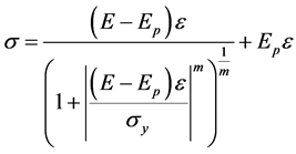 , (12)
 , (13)
where  is the effective strain hardness, which is set to
  in our numerical experiments;
 ![]() is a parameter that controls the degree of smoothness, which is set at
is a parameter that controls the degree of smoothness, which is set at , close to bilinear point; and
  is the tangential stiffness at an arbitrary point [8] .
The tangent stiffness matrix for the three-dimensional truss takes the form
 , (14)
where
 , (15)
 , (16)
 . (17)
Here  is the axial force,
  and
and  are the indices of the nodes at the segment endpoints,
  and
and  are the
 ![]() coordinates of nodes
coordinates of nodes , and
, and ![]() is the segment length.
is the segment length.
Figure 3 plots the load-displacement curve obtained using the proposed method. Figures 3 and 4 indicate the correct count of eigenvalues. A total of six eigenvalues appear before the limit point, with the sixth eigenvalue corresponding to the limit point itself. ![]() through
through  are bifurcation buckling points, and
  is the limit point. The pair
  is a pair of multiple roots, as is the pair
 . If the number
 ![]() of subdivisions for the strain value constraint is too small, discrepancies in the number of zero eigenvalues detected by the proposed method can arise, causing some singular points to be overlooked. For this reason, we have here chosen
of subdivisions for the strain value constraint is too small, discrepancies in the number of zero eigenvalues detected by the proposed method can arise, causing some singular points to be overlooked. For this reason, we have here chosen , but high-precision nonlinear analyses require large numbers of steps. The method that we have proposed is a simple addition to the process of solving simultaneous linear equations and may be put to effective use in nonlinear analysis.
5. Conclusions
We have presented a formula for computing the derivative of a determinant with respect to an eigenvalue. Our computation proceeds simultaneously with the modified Cholesky  decomposition of the matrix, a characteristic example of a direct solution method. We applied our proposed formula to the determination of singular points, such as branch points and breaking points, in the arc-length method in a nonlinear finite-element
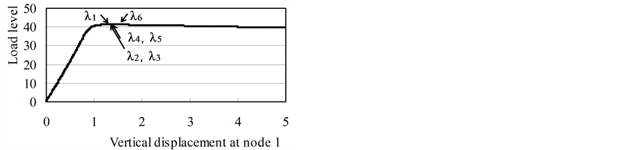
Figure 3. Vertical displacement and load level.
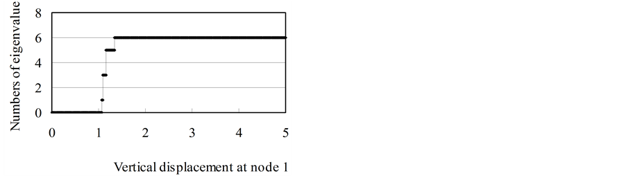
Figure 4. Vertical displacement and numbers of eigenvalue.
method. In this application, we detect changes in the sign of the derivative of the determinant and then use the bisection method to narrow the interval containing the singular point.
Moreover, because the solution obtained via the Newton-Raphson method varies with the derivative of the determinant, it is possible to use this quantity as the arc length. This then allows the arc-length increment to be determined automatically, which in turn allows a reduction in the number of basic parameters impacting the nonlinear analysis. However, as our numerical experiments demonstrated, when using the proposed method, it is necessary to impose a constraint on the absolute value of the maximum values of the strain or the relative strain, and to use the strain constraint to control the increment. The proposed method is designed to work with the  decomposition and exhibits a significant reduction in memory requirements when applied to the
  decomposition of banded matrices instead of dense matrices.
Numerical experiments on a three-dimensional truss structure demonstrated that the proposed method is able to identify singular points (bifurcation points and limit points) accurately using the derivative with respect to an eigenvalue of the characteristic equation of the stiffness matrix. This method does not require the time-consuming step of solving the eigenvalue problem and makes use of the solution to the simultaneous linear equations arising in incremental analysis, thus making it an extremely effective technique.
References
- Kashiwagi, M. (1999) An Eigensolution Method for Solving the Largest or Smallest Eigenpair by the Conjugate Gradient Method. Transactions of JSCES, 1, 1-5.
- Kashiwagi, M. (2009) A Method for Determining Intermediate Eigensolution of Sparse and Symmetric Matrices by the Double Shifted Inverse Power Method. Transactions of JSIAM, 19, 23-38.
- Kashiwagi, M. (2008) A Method for Determining Eigensolutions of Large, Sparse, Symmetric Matrices by the Preconditioned Conjugate Gradient Method in the Generalized Eigenvalue Problem. Journal of Structural Engineering, 73, 1209-1217.
- Kashiwagi, M. (2011) A Method for Determining Intermediate Eigenpairs of Sparse Symmetric Matrices by Lanczos and Shifted Inverse Power Method in Generalized Eigenvalue Problems. Journal of Structural and Construction Engineering: Transactions of AIJ, 76, 1181-1188. http://dx.doi.org/10.3130/aijs.76.1181
- Kashiwagi, M. (2013) Derivative of a Determinant with Respect to an Eigenvalue in the LDU Decomposition of a Non-Symmetric Matrix. Applied Mathematics, 4, 464-468. http://dx.doi.org/10.4236/am.2013.43069
- Bathe, K.J. (1982) Finite Element Procedures in Engineering Anaysis, Prentice-Hall, Englewood Cliffs, Nj.
- Fujii, F. and Choong, K.K. (1992) Branch Switching in Bifurcation of Structures. Journal of Engineering Mechanics. 118, 1578-1596. http://dx.doi.org/10.1061/(ASCE)0733-9399(1992)118:8(1578)
- Richrd, R.M. and Abotto, B.J. (1975) Versatile Elastic-Plastic Stress-Strain Formula. Journal of Engineering Mechanics. 101, 511-515.