American Journal of Operations Research
Vol. 2 No. 2 (2012) , Article ID: 19934 , 10 pages DOI:10.4236/ajor.2012.22021
A Production Inventory Model with Shortages, Fuzzy Preparation Time and Variable Production and Demand*
1Department of Mathematics, Panskura Banamali College, Panskura, India
2Department of Mathematics, Bengal Institute of Technology & Management, Santiniketan, India
3Department of Applied Mathematics, Vidyasagar University, Midnapore, India
Email: {nirmal_hridoy, bera_uttam, mmaiti2005}@yahoo.co.in
Received February 8, 2012; revised March 10, 2012; accepted March 26, 2012
Keywords: Fuzzy Preparation Time; Interval Number; Multi-Objective; Global Criteria Method
ABSTRACT
A production inventory model is formulated for a single item. Here, demand varies with the on-hand inventory level and production price. Shortages are allowed and fully backlogged. The time gap between the decision and actual commencement of production is termed as “preparation time” and is assumed to be crisp/imprecise in nature. The set-up cost depends on preparation time. The fuzzy preparation time is reduced to a crisp interval preparation time using nearest interval approximation and following the interval arithmetic, the reduced problem is converted to a multi-objective optimization problem. Mathematical analysis has been made for single objective crisp model (Model-I). Numerical illustration have been made for both crisp (Model-I) and fuzzy (Model-II) models. Model-I is solved by generalized reduced gradient technique and multi-objective model (Model-II) by Global Criteria Method. Sensitivity analyses have been made for some parameters of Model-I.
1. Introduction
After the development of EOQ model by Harris [1] in 1915, a lot of researchers have extended the above model with different types of demands and replenishment. A detailed literature is available in the text book such as Hadley and Whitin [2], Tersine [3], Silver and Peterson [4], etc. In classical inventory models, demand is normally assumed to be constant. But, now-a-days, with the invasion of the multi-nationals under the WTO agreement in the developing countries like India, Bangladesh, etc., there is a strong competition amongst the sellers to capture the market i.e. to allure the customers through different tactics. Common practices in this regard is to have attractive decorative gorgeous display of the items in the show room to create psychological pressure or to motivate the customers to buy more. Furthermore, demand of an item depends on unit production cost, i.e. it varies inversely with the unit production cost. This marketing policy is very useful for fashionable goods/fruits etc. There is some literature on the inventory models with stock-dependent demand. Several authors like Mandal and Phaujdar [5], Urban [6], Bhunia and Maiti [7], and others studied the above-mentioned type of inventory models.
Existence of Lead-time (the time gap between placement of order and the actual receipt of it) is a natural phenomenon in the field of business. So far, most of the researchers have dealt with either constant or stochastic lead-time. Elementary discussion on lead-time analysis are now-a-days available in the textbooks like Naddor [8], Magson [9], Foote, Kebriaci and Kumin [10] and others. In practice, it is difficult to predict the lead-time definitely/pricelessly and sometimes, the past records are also not available to form a probability distribution for the lead-time. Hence, the only alternative available to DM is to define the lead-time parameter imprecisely by a fuzzy number. Generally, lead time is associated with EOQ model i.e. instantaneous procurement or purchase of the lot. But, in a production system,the scenario is different. Here the time gap between the decision production and the actual commencement of production matters known as preparation time for the analysis of inventory control models. This preparation time means the time to collect the raw-materials, to arrange skilled/unskilled labors, to get machine ready for production, etc., and hence influences the set-up cost of the system. For the first time, Mahapatra and Maiti [11,12] formulated and solved production inventory models for a deteriorating/breakable item with imprecise preparation time.
Though multiobjective decision making (MODM) problems have been formulated and solved in many other areas like air pollution, structural analysis (cf. Rao [13]), transportation (cf. Li and Lai [14]), etc., till now few papers on MODM have been published in the field of inventory control. Padmanabhan and Vrat [15] formulated an inventory problem of deteriorating items with two objectives—minimization of total average cost and wastage cost in crisp environment (It is an environment where all input data are assumed to be deterministic, precisely defined and given.) and solved by non-linear goal programming method. Roy and Maiti [16] formulated an inventory problem of deteriorating items with two objectives, namely, maximizing total average profit and minimizing total waste cost in fuzzy environment. Mahapatra, Roy and Maiti [17], Mahapatra, Das, Bhunia and Maiti [18] formulated multi-objective multi-item inventory problems under some constraints.
In this paper, a production inventory control system for a single item is considered. Here demand is dependent on unit production cost and current stock level. Shortages are allowed and backlogged fully. Preparation time in production of the new consignment is allowed and crisp/fuzzy in nature. The setup cost is dependent on preparation time. The crisp problem for minimizing average cost is solved by generalized reduced gradient method. The problem minimizing average total cost with fuzzy preparation time is converted to a multi-objective minimization problem with the help of interval arithmetic and then it is solved by global criteria method to get pareto-optimal solution. Mathematical derivation and analysis also have been made for both single and multiobjective models. Further, the sensitivity analysis is included and two numerical illustration are provided.
2. Interval Arithmetic
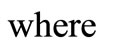
Throughout this section lower and upper case letters denote real numbers and closed intervals respectively. The set of all positive real numbers is denoted by . An order pair of brackets defines an interval
  where
where  and
and  are respectively left and right limits of
 .
.
Definition 2.1: Let  be a binary operation on the set of positive real numbers. If
  and
and  are closed intervals then
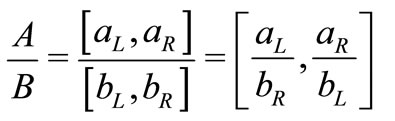
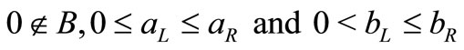
  defines a binary operation on the set of closed intervals. In the case of division, it is assumed that
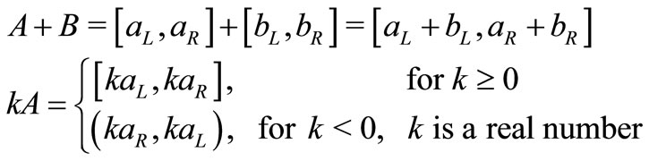
 . The operations on intervals used in this paper may be explicitly calculated from the above definition as
2.1. Order Relations between Intervals
Here, the order relations which represent the decisionmaker’s preference between interval costs are defined for minimization problems. Let the uncertain costs for two alternatives be represented by intervals A and B respectively. It is assumed that the cost of each alternative is known only to lie to the corresponding interval. The order relation by the left and right limits of interval is defined in Definition-2.2.
Definition 2.2: The order relation  between
 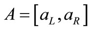 and
and 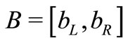 is defined as
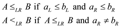
The order relation  represents the DM’s performance for the alternative with the lower minimum cost, that is, if
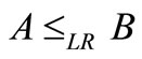 , then
  is preferred to
 .
.
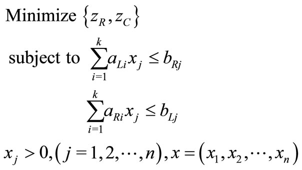
2.2. Formulation of the Multi-Objective Problem
A general non-linear objective function with some interval valued parameters is as follows:
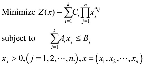 (1)
(1)
where 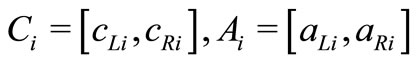 and
and 
Now, we exhibit the formulation of the original problem (1) as a multi-objective non-linear problem. Since the objective function  and the constraints contain some parameters represented by intervals, it is natural that the solution set of (1) should be defined by preference relations between intervals.
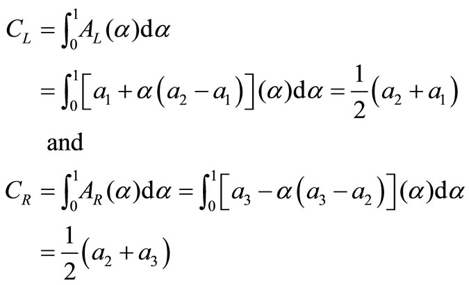
Now from Equation (1) the right and left limits  and centre
  of the interval objective function
  respectively may be elicited as
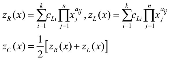
Thus the problem (1) is transformed into
2.3. Basic Fuzzy Sets and Fuzzy Numbers
Fuzzy set: A Fuzzy set  in a universe of discourse
  is defined as the following set of pairs
 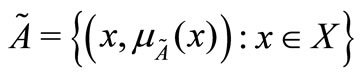 , where
 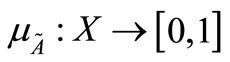 is a mapping called the membership function of the fuzzy set
  and
and  is called the membership value or degree of membership of
  in the fuzzy set
 . The larger
  is the stronger grade of membership form in
 .
.
Fuzzy number: A fuzzy number is a fuzzy set in the universe of discourse  that is both convex and normal. Figure 1 shows a fuzzy number
  of the universe of discourse
  that is both convex and normal.
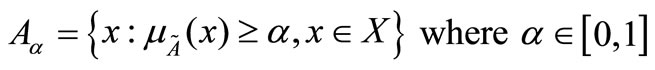
 -cut of a fuzzy number: The
  -cut of a fuzzy number
  is defined as crisp set
 is a non-empty bounded closed interval contained in
  and it can be denoted by
 .
.  and
and  are the lower and upper bounds of the closed interval respectively.
Figure 1 shows a fuzzy number  with
with  -cuts
-cuts . It is seen that if
  then
then  and
and  .
.
Fuzzy numbers are represented by two type of membership functions: 1) Linear membership functions e.g. Triangular fuzzy number (TFN), Trapezoidal fuzzy number, Piecewise Linear fuzzy number etc. 2) Non-linear membership functions e.g. Parabolic fuzzy number (PFN), Parabolic flat fuzzy number, Exponential fuzzy number and other non-linear fuzzy number.
2.4. Triangular Fuzzy Number (TFN)
TFN is the fuzzy number with the membership function , a continuous mapping :
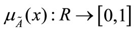
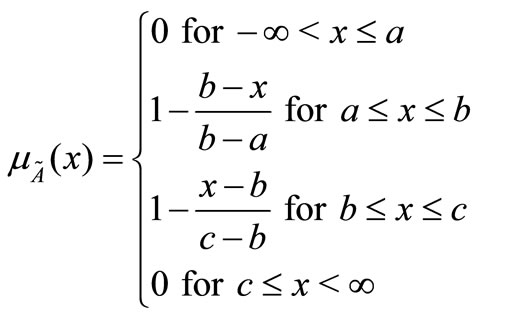
Figure 2 shows a Triangularm fuzzy number  of the universe of discourse
  that is both convex and normal.
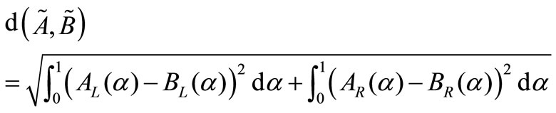
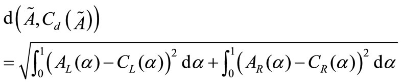
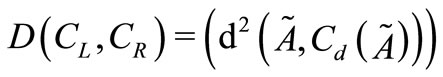
2.5. The Nearest Interval Approximation
Here we want to approximate a fuzzy number by crisp one. Suppose  and
and  are two fuzzy numbers with
  -cuts are
  and
and  respectively. Then the distance between
  and
and  is
is
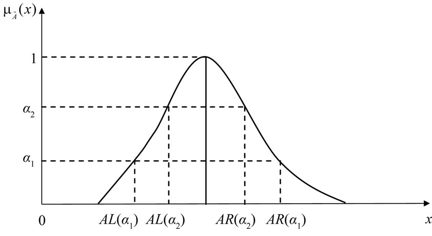
Figure 1. Fuzzy number  with α-cuts.
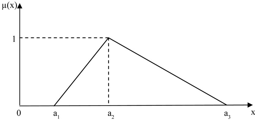
Figure 2. Triangular fuzzy number.
Given  is a fuzzy number. We have to find a closed interval
  which is nearest to
  with respect to metric
 . We can do it since each interval is also a fuzzy number with constant
  -cut for all
 . Hence
 . Now we have to minimize
with respect to  and
and . In order to minimize
 , it is sufficient to minimize the function
 . The first partial derivatives are
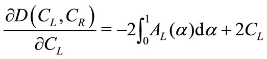
and 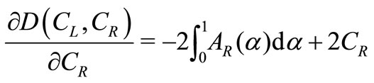
Solving 
we get  and
and .
.
Again since
So  i.e.
i.e.  is global minimum. Therefore the interval
is nearest interval approximation of fuzzy number  with respect to metric
 . Let
. Let  be a fuzzy number. The α-level interval of
  is defined as
 .
.
When  is a TFN then
 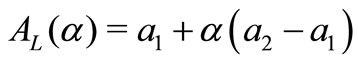 and
and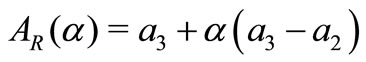 .
.
By nearest interval approximation method lower and upper limits of the interval are respectively
Therefore, interval number considering  as a TFN is
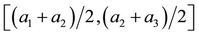 .
.
3. Assumptions and Notations for the Proposed Model
The following notations and assumptions are used in developing the model.
1) Production system involves only one non-deteriorating item.
2) Shortages are allowed and fully backlogged.
3) Time horizon is infinite.
4)  = inventory level at any time
 .
.
5)  = the maximum inventory (shortages) level in an cycle.
6)  = preparation time for the next production,which is a fuzzy number.
7)  = Set-up cost which is of the form
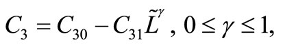
 and
and  are two constants so chosen to best fit the set-up cost.
8)  = production cost per unit item.
9)  = Rate of demand which depends on production price and stock i.e.,
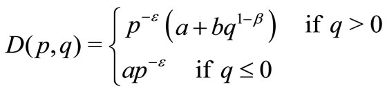
where  are positive real constants.
10)  = cycle length of a cycle.
11)  = holding cost per unit per unit time.
12)  = shortage cost per unit per unit time.
13)  = re-production time, i.e., time when production for next cycle is decided.
14)  = production rate which is of the form
  and
and .
.
4. Mathematical Formulation
Production inventory system involves only one item. A cycle starts with shortages at time  and at time
  maximum shortages level is
  and at that time production process starts to backlog the shortage quantities fully and after time
  the shortages reached to zero, inventory accumulates up to time
  of amount
 . At that time production process stopped, accumulated inventory declines due to demand and reaches to zero at time
 . The above production inventory system is shown in Figure 3. The differential equations governing the stock status for this model are given by
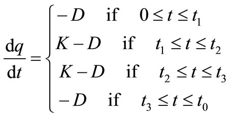 (2)
(2)
with the boundary conditions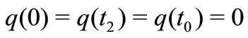 . These equations can be rewritten in the following form.
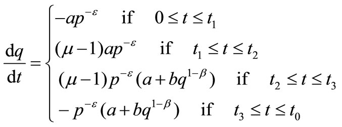 (3)
(3)
For simplicity we take . Solving first and second equations of differential Equation (3) in the intervals
  and
and  respectively with the help of boundary conditions
 , we get
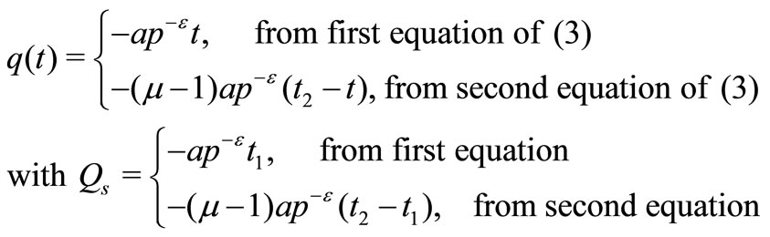
So at time ,
,
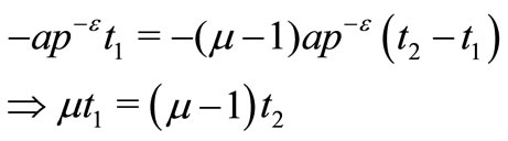
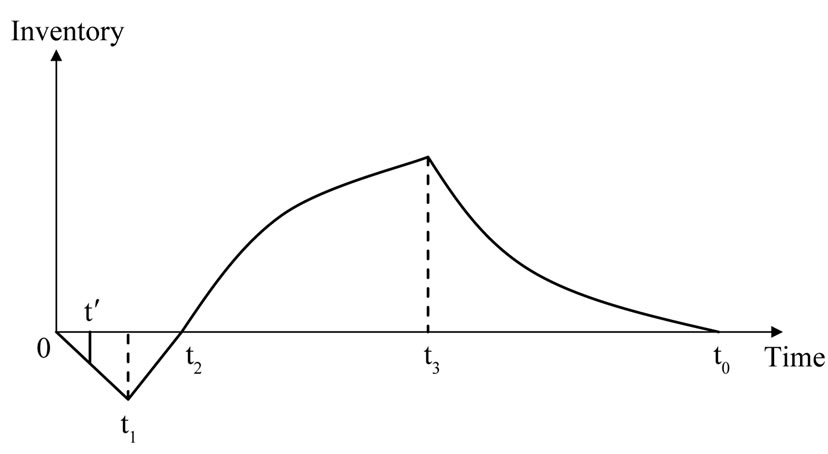
Figure 3. Inventory begins with backlogged shortages and end with no inventory.
Similarly, solving third and fourth differential Equations of (8) in the interval  and
and  respectively with the help of the boundary conditions
 , we get
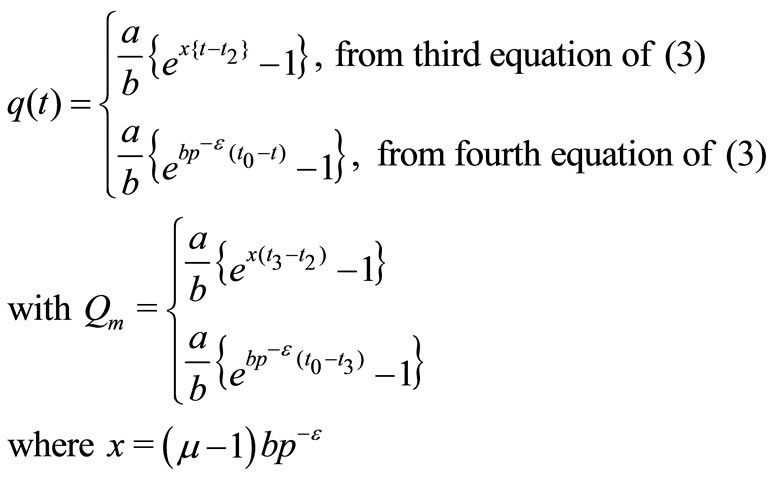 (5)
(5)
At time ,
,
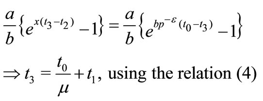 (6)
(6)
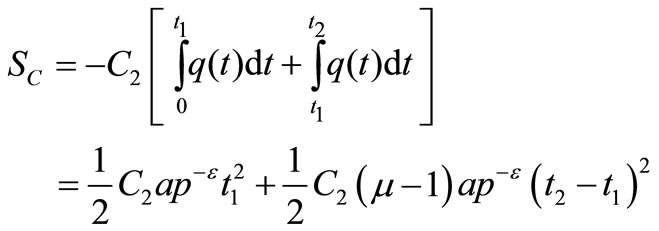
Total shortages cost  is given by
Now the total holding cost ( ) during the interval
 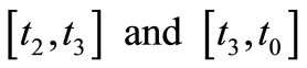 is given by
Total production cost 
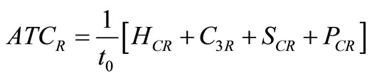
Now the average total cost 
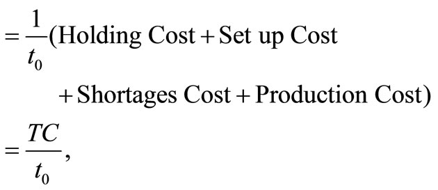
where
4.1. Crisp Model (Model-I)
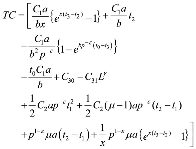
Hence, the proposed model can be stated as
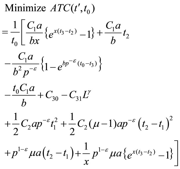 (7)
(7)
4.2. Fuzzy Model (Model-II)
As in this case, preparation time is a fuzzy number  which is replaced by an appropriate interval number
  and so, in this case
  is replaced by
  (for details see Appendix I) and the crisp problem (7) becomes a fuzzy optimization problem which, using interval arithmetic, becomes a multi-objective nonlinear programming problem as follows:
 (8)
(8)

 .
.
5. Mathematical Analysis
5.1. Model-I (Crisp Model)
The objective function ATC of Model-I is a function of  and
and  as
as  and
and  are dependent variable (depend on
  and
and ). To achieve optimal
  and
and , the partial derivatives of the average total cost ATC with respect to
  and
and  are set to zero. The resulting equation can be solved simultaneously to obtain the optimal
  and
and .
.
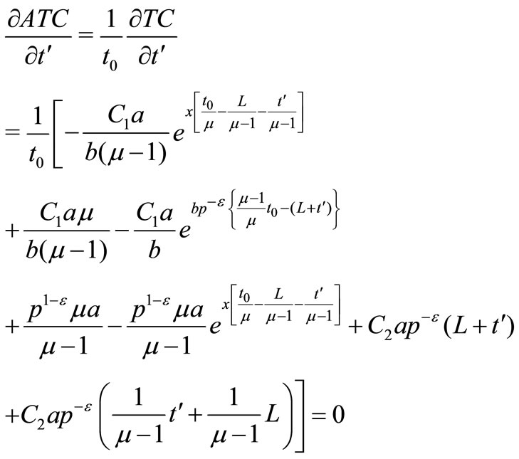 (9)
(9)

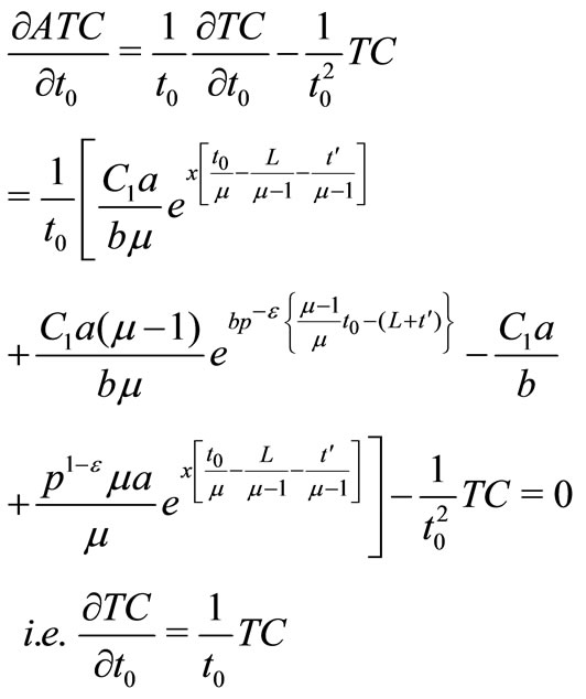 (10)
(10)
ATC can be proved as strictly convex since all the principal minors of its Hessian matrix are strictly positive.
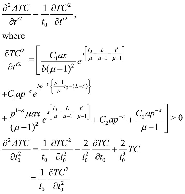 (11)
(11)
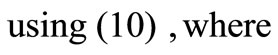
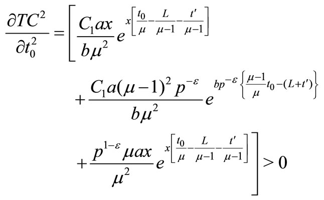 (12)
(12)
and

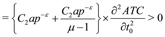
Hence, the solution of Model-I is global minimum of .
.
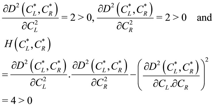
5.2. Model-II (Fuzzy Model)
In Model-II, the objective functions  and
and  (and hence
 ) are functions of
  and
and  as
as  and
and  are dependent variable (depend on
  and
and ). As of Model-I, it can be seen that
  and
and  (and hence
 ) are strictly convex.
Definition 5.1: A multi-objective optimization problem is convex if all the objective functions and the feasible region are convex.
Definition 5.2:  is said to be a Pareto optimal solution to the MONLP iff there does not exist another
  in the feasible region such that
  for all
  and
and  for at least one index
An objective vector  is Pareto-optimal if there does not exist another objective vector
  such that
  for all
  and
and  for at least one index
 . Therefore,
  is Pareto-optimal if the decision vector corresponding to it is Pareto optimal.
Theorem 5.1: Let the multi-objective optimization problem be convex. Then every locally Pareto-optimal solution is also globally Pareto-optimum (cf. Miettinen [19])).
Therefore the problem given by (7) is a strictly convex multi-objective minimization problem and hence possesses global Pareto-optimal solutions. Hence, the problem (7) is solved by Global Criteria Method.
5.3. Global Criteria Method
The Multi-Objective Non-linear Programming (MONLP) problems are solved by Global Criteria Method converting it to a single objective optimization problem. The solution procedure is as follows.
• Step-1. Solve the multi-objective programming problem (16) as a single objective problem using only one objective at a time ignoring.
• Step-2. From the above result, formulate a pay-off matrix as follows:
• Step-3. From the pay-off matrix of Step-2, determine the ideal objective vector, say  and the corresponding value of
 .
.
Here, the ideal objective vector is used as a reference point. The problem is then to solve the following auxiliary problem:
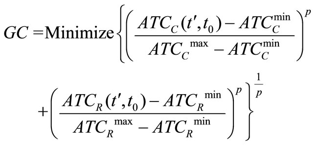 (13)
(13)
where  and GC is known as global criteria. An usual value of p is 2.
6. Numerical Illustrations
6.1. Crisp Model (Model-I)
The Equation (7) is non-linear in  and
and  and difficult to obtain the optimal values of
  and
and  by Calculus method. Hence, we minimize (7) by a gradient based non-linear optimization method. Using the optimal values of
  and
and , the corresponding values of
  and minimum average total cost (ATC) are be obtained. To illustrate the proposed inventory model (Model-I), following input data are considered.
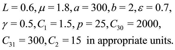
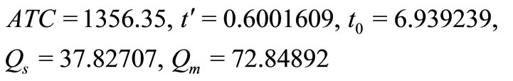
Solving the Model-I, following optimal values are obtained:
6.2. Fuzzy Model (Model-II)
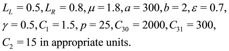
To illustrate the proposed inventory Model-II, following input data are considered.
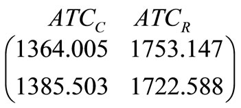
For the above input data, formulate a pay-off matrix as follows:
Solving the Model-II using Global Criteria Method, following optimal values are obtained:
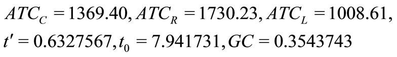 .
.
7. Discussion
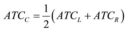
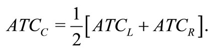
The Model-I is a single objective optimization problem and is solved using generalized reduced gradient method. The Model-II is a multiobjective problem and is solved by Global Criteria Method. In Model-II, the average cost minimization problem with interval objective function was converted into the multi-objective problem whose objectives are to minimize the centre ( ) and right limit (
 ) of the interval objective function. These two objective functions can be considered as the minimization of the average case and the worst case. The solution sets of production inventory problems with interval objective functions are defined as the Pareto optimal solutions of the corresponding multi objective problem. Therefore, the solution set defined in this paper includes the optimal solutions against both the worst and the average cases.
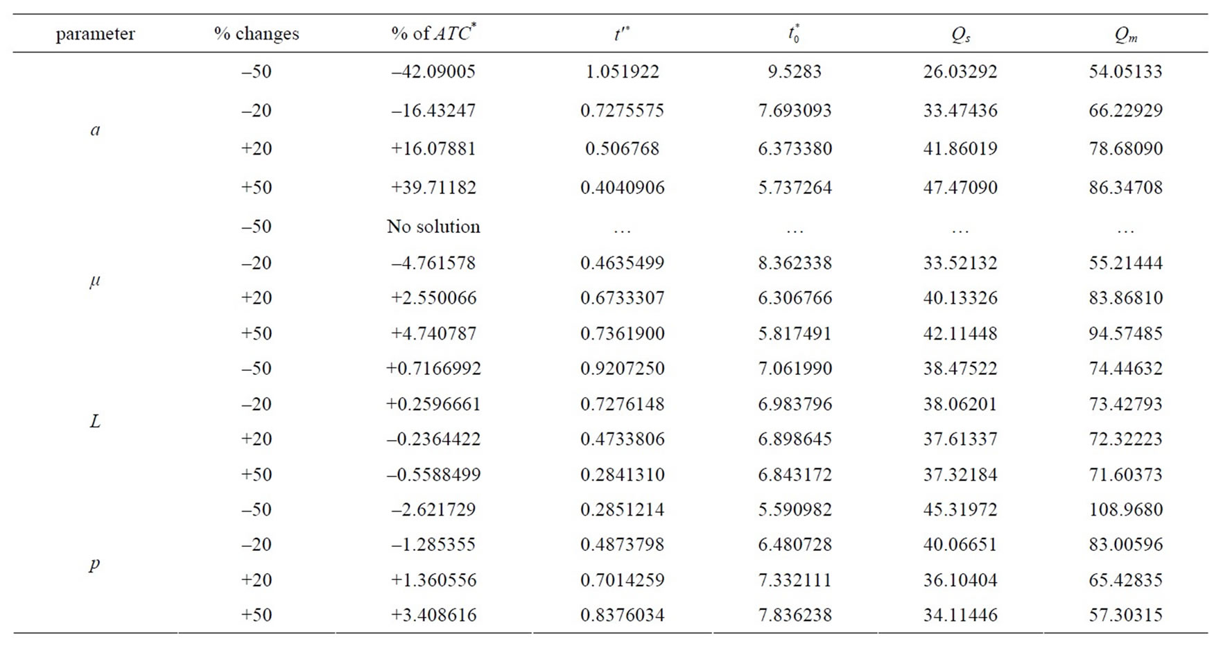
Table 1. Sensitivity analysis of Model-I.
8. Sensitivity Analysis
A sensitivity analysis of the decision variables  and
and  for Model-I have been made when each of the parameters
  being changed from
  to
to . The relative change of
  are also taken into account and presented in Table 1. From Table 1, it is seen that
  changes rapidly with the rapid change of the parameter a, but these change are too slow in case of parameter
  and p. Again,
  increases and decreases with decrease and increase in preparation time
  respectively, but this change is slow which agrees with the real phenomenon.
Figure 4 shows the  versus b graph. From this graph it is revealed that initially
  decreases rapidly with the increase in b and after some time it begins to increase slowly. Here, it is interesting to note the effect of shape parameter b of the demand function on
 .
.
9. Practical Implications
In this preparation time has been considered for an inventory model with finite production rate. In real life, once production is discontinued, i.e., once the labour force is dismantled, supply of raw materials is disrupted, machineries is kept in disorder, etc., it is obvious that to start the next production, some time is required to bring the above mentioned things in order. The cost related to above factors depends on the time gap between the decision to start the preparation and actual commence of production. If the gap is small, then everything will have to be arranged hurriedly and it costs more. Hence, setup
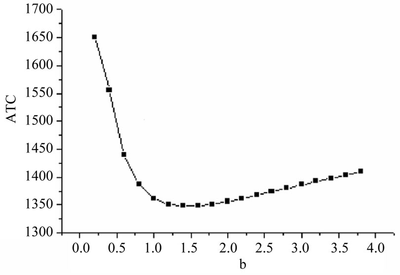
Figure 4. Graph of ATC versus b.
cost decreases with the increase of preparation time. The preparation time for the next production run is very important. This decision influences several costs like setup cost, production cost, etc. Such real life models are considered here taking different environments into consideration.
The fuzzy numbers are described by linear/non-linear type membership functions. Fuzzy number describing preparation time is then approximated to an interval number. Following this, the fuzzy problem is converted into multi-objective inventory problem where the objective functions are represented by right limit and centre of interval function which are to be minimized. The proposed model has a broad area of applicability. Two inventory models are presented with different type of preparation time. If a decision maker (DM) knows definitely the time required to restart the next production run, he/ she may adopt Model-I. Similarly, for fuzzy preparation time, DM may accept the Model-II. DM may select any of these models according to the prevailing environment in his/her production centre.
10. Conclusions
The present paper proposes a solution procedure for production inventory model with production cost and on hand inventory dependent demand rate and preparation time. Here, shortages are allowed and backlogged fully. Like lead time, time when the decision is taken for the preparation of next production run i.e. preparation time has been considered for a production inventory model. In real life, setup cost decreases with the increase of preparation time. This consideration is taken into account in Model-I. In Model-II, preparation time is taken as imprecise via a fuzzy number. The fuzzy number is described by linear/non-linear type membership function.
Fuzzy number describing preparation time is then approximated to an interval number. Following this, the problem is converted into multi-objective inventory problem where the objective functions are represented by centre and right limit of interval function which are to be minimized. To obtain the solution of the multi-objective inventory problem, Global Criteria Method has been used. The proposed demand has a broad area of applicability. Demand of a commodity decreases with the increase in production cost but increases with the increase of stock of the displayed commodity and vice versa. Here, though the formulation of the model and the solution procedure are quite general, the model is a simple production model with demand dependent production rate. The unit production cost which is assumed here to be constant, in reality, varies with the preparation time and produced quantity. Moreover, time dependent production rate, partially lost sales, inflation, etc., can be incorporated to the model to make it more realistic. Here, demand is stockdependent. The present analysis can be repeated for the dynamic demand also. Though the problem has been presented in crisp and fuzzy environment, it can also be formulated and solved in fuzzy-stochastic environment representing production cost and inventory costs through probability distribution.
REFERENCES
- F. Harris, “Operations and Cost (Factory Management Series),” A.W. Shaw Co., Chicago, 1915, pp. 48-52.
- G. Hadley and T. M. Whitin, “Analysis of Inventory Systems,” Prentice Hall, Englewood Cliffs, 1963.
- R. J. Tersine, “Principles of Inventory and Materials Management,” Elsevier North Holland Inc., New York, 1982.
- E. A. Silver and R. Peterson, “Decision System for Inventory Management and Research,” John Wiley, New York, 1985.
- B. N. Mandal and S. Phaujdar, “A Note on Inventory Model with Stock-Dependent Consumption Rate,” OPSEARCH, Vol. 26, 1989, pp. 43-46.
- T. L. Urban, “Deterministic Inventory Models Incorporating Marketing Decisions,” Computer and Industrial Engineering, Vol. 22, No. 1, 1992, pp. 85-93. doi:10.1016/0360-8352(92)90035-I
- A. K. Bhunia and M. Maiti, “An Inventory Model for Decaying Items with Selling Price, Frequency of Advertisement and Linearly Time Dependent Demand with Shortages,” IAPQR Transactions, Vol. 22, 1997, pp. 41- 49.
- E. Naddor, “Inventory System,” John Wiley, New York, 1966.
- D. Magson, “Stock Control When Lead-Time Can Not Be Considered Constant,” Journal of the Operational Research Society, Vol. 30, 1979, pp. 317-322.
- B. Foote, N. Kebriaci and H. Kumin, “Heuristic Policies for Inventory Ordering Problems with Long and Random Varying Lead Times,” Journal of Operations Management, Vol. 7, No. 3-4, 1988, pp. 115-124. doi:10.1016/0272-6963(81)90008-5
- N. K. Mahapatra and M. Maiti, “Inventory Model for Breakable Item with Uncertain Preparation Time,” Tamsui Oxford Journal of Management Sciences, Vol. 20, No. 2, 2004, pp. 83-102.
- N. K. Mahapatra and M. Maiti, “Production-Inventory Model for a Deteriorating Item with Imprecise Preparation Time for Production in Finite Time Horizon,” Asia Pacific Journal of Operations Research, Vol. 23, No. 2, 2006, pp. 171-192.
- S. S. Rao, “Multi Objective Optimization in Structural Design with Uncertain Parameters and Stochastic Process,” AIAA Journal, Vol. 22, 1984.
- L. Li and K. K. Lai, “A Fuzzy Approach to the Multiobjective Transportation Problem,” Computers & Operations Research, Vol. 27, No. 1, 2000, pp. 43-57. doi:10.1016/S0305-0548(99)00007-6
- G. Padmanabhan and P. Vrat, “EOQ Models for Perishable Items under Stock-Dependent Selling Rate,” European Journal of Operations Research, Vol. 86, No. 2, 1995, pp. 281-292. doi:10.1016/0377-2217(94)00103-J
- T. K. Roy and M. Maiti, “Multi-Objective Inventory Models of Deteriorating Items with Some Constraints in a Fuzzy Environment,” Computers and Operations Research, Vol. 25, No. 12, 1998, pp. 1085-1095. doi:10.1016/S0305-0548(98)00029-X
- N. K. Mahapatra, T. K. Roy and M. Maiti, “Multi-Objective Multi-Item Inventory Problem,” Proceedings of the Seminar on Recent Trends and Developments in Applied Mathematics, Howrah, 3 March 2001, pp. 44-68.
- N. K. Mahapatra, K. Das, A. K. Bhunia and M. Maiti, “Multiobjective Inventory Model of Deteriorating Items With Ramp Type Demand Dependent Production, Setup and Unit Costs,” Proceedings of the National Symposium on Recent Advances of Mathematics and Its Applications in Science and Society, University of Kalyani, Kalyani, 21-22 November 2002, pp. 89-110.
- K. M. Miettinen, “Non-Linear Multi-Objective Optimization,” Kluwer’s International Series, Boston, 1999.
Appendix I
Since preparation time is a fuzzy number which is replaced by an appropriate interval number , therefore from Equations (4) and (6), replacing
  by
by , we have
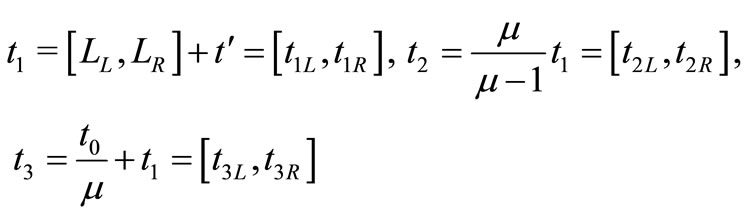
where
Total shortages cost  is given by
where
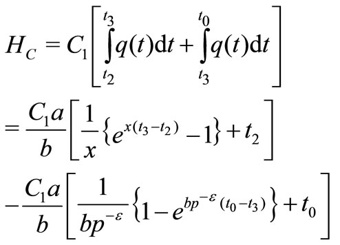
Now the Set-up cost  is given by
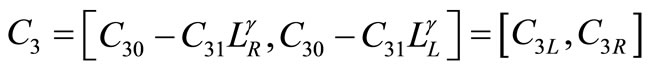 .
.
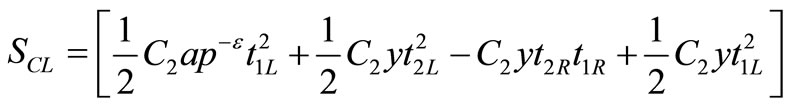
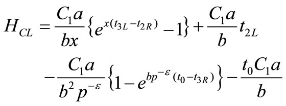
Now the total holding cost ( ) during the interval
  is given by
where
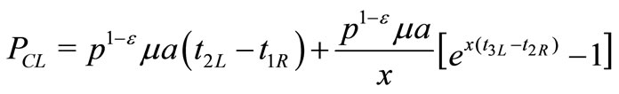
Total Production cost is given by
where
Now the expressions of  and
and  may be obtained from the expressions of
  and
and  on replacing the suffices
  by
by  and
and  by
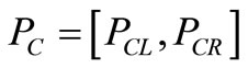
by  respectively. Therefore, the total cost becomes
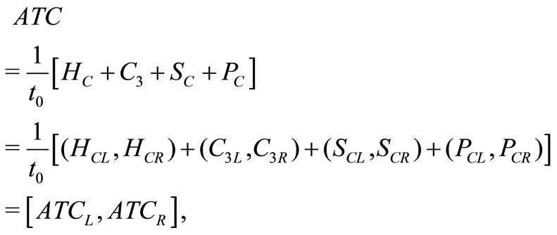
where
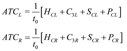
and
NOTES
*This work is supported by University Grants Commission, Govt. of India under the research grand No. F.PSW-096/05-06 (ERO).