Journal of Analytical Sciences, Methods and Instrumentation
Vol.2 No.3(2012), Article ID:23283,4 pages DOI:10.4236/jasmi.2012.23024
Guided Waves Mode Discrimination in Pipes NDT Based on the Matching Pursuit Method
![]()
College of Architecture and Power, Naval University of Engineering, Wuhan, China.
Email: *wangde99@hotmail.com
Received July 4th, 2012; revised August 6th, 2012; accepted August 15th, 2012
Keywords: Guided Waves Modes; Discrimination; Matching Pursuit; Pipes Nondestructive Testing
ABSTRACT
Ultrasonic guided wave have the multi-modes and dispersive characteristics, and its modes are easy to be converted at boundary or when running into defects in pipes, which makes the discrimination of different guided waves modes of the reflection signals in pipes NDT very hard. In this work, firstly, the experiments are carried out to test two kinds of stainless steel pipes by applying guided waves NDT, one is integrated pipe and another is non-integrated pipe with a small hole defect, and the detected guided waves echo signals are respectively obtained. Secondly, the measured signals are processed by matching pursuit method and the Chirplet matching atom parameters are calculated. By calculating the time-frequency distributions spectrum of detected guided waves echo signals, torsional, flexural and longitudinal guided waves modes are identified from the intact pipe, and the two wave-packets with torsional and flexural guided waves modes are also identified from the pipe with hole defect. The results showed that the matching pursuit method has a tremendous advantage to identify different guided waves modes in pipes nondestructive testing.
1. Introduction
It is very important to identify different guided waves modes for ultrasonic guided waves NDT to diagnose the structure integrity. Traditional guided waves signal processing methods include the wave-form analysis such as wavelet analysis [1] in the time domain, the two dimensional Fourier Transform [2] in the frequency domain and the short Time Fourier Transform [3] in the timefrequency domain. Recently, correlation analysis [4] and Duffing chaotic oscillator [5] have been applied to identify the small flaw and improved the accuracy of fault detection by guided wave inspection. A Fourier basis provided a poor representation of functions well localized in time, and wavelet basis are not well suitable to represent functions whose fourier transforms have a narrow high frequency support. In both cases, it is difficult to detect and identify the guided wave patterns from their expansion coefficients, because the information is diluted across the whole basis. The wavelet analysis, correlation analysis and duffing chaotic oscillator can be used as different kinds of denoise approaches and they can not identify the different guided wave modes. The Fourier Transform can only get the frequency information. The short Time Fourier Transform can get the guided wave modes but it can only identify the modes in a narrow frequency domain [3].
The Matching Pursuit method (MP) [6] has an advantage of decomposing any signal into a linear expansion of waveforms that are selected from a redundant dictionary of functions, and these waveforms are chosen in order to best match the signal structures. The signal processed by MP makes sure that the signal’s frequency and time domain information can be reserved. MP is a kind of iteractive algorithm to adaptive compute signal representations. With a dictionary of Gabor functions, MP defines an adaptive time-frequency transform, and isolates the signal structures that are coherent with respect to a given dictionary. MP have been used in signal processing such as ultrasonic [7], radar [8] and guided wave [9], and fuzzy clustering and classification of signals [10,11]. The modified MP have been used in the field of ultrasonic signal processing such as flaw echo detecting [12] and feature extraction [13], and electroencephalogram (EEG) recognition [14]. Peng Xu proposed a kind of two dictionaries matching pursuit (TDMP) to decompose and reconstruct signals which can reduce the computation load [15]. Jin-Chul Hong proposed a chirp dictionarybased matching pursuit approach to estimate the location and size of a crack from longitudinal wave signals measured in cracked rod, which shows that this approach is very useful [16]. In addition, MP can be applied to guided waves modes extraction and identification. Ajay Raghavana [17] applied Chirplet matching pursuits to process guided waves signals and distinguish overlapping multi-mode signals of lamb waves in plate structures. Fucai Li distinguished the mode of each lamb wave package and pinpoint these packages for estimating the actual group velocities of dispersion curves and localizing damage by using ridge in the time-scale domain [18].
In this work, MP is applied to process and identify different guided waves modes signals (Longitudinal, Torsional and Flexual modes) for pipe structures nondestructive testing by choosing Chirplet function as matching atoms, analyzing and comparing the Wigner-Ville distribution of the extracted wave packages to the guided wave dispersion curves.
2. Matching Pursuit Method and the Selection of Matching Atoms
2.1. Matching Pursuit Method
To decompose the signal  by the matching pursuit method, firstly , an over-complete dictionary of waveforms D (
 ) is determined, and a best match waveform or“atom”
  is selected from the dictionary, which makes the absolute value of the inner product
  maximum in some extent [6]. We can get
  by subtracting the contribution of atom
  from the signal
 . The signal
  can be decomposed as
 (1)
(1)
The process is repeated on the residual . After the nth iteration we can get
 .
.
 (2)
(2)
Subsequently, the signal  will be decomposed into the sum as:
 (3)
(3)
It has been proved that the norm of residual  decay to zero exponentially when n inclines to infinite. In application to signal decomposition, the decomposition process will stop when
  reaches a predefined threshold. Then the signal
  can be expressed as:
 (4)
(4)
2.2. Selection of Matching Atoms
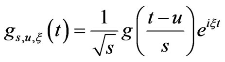
According to the matching pursuit method, an overcomplete dictionary of atoms should be determined to match the characters of guided waves pulse echo signals, so that the signal decomposition can be highly sparse and compacted. Generally, Gabor functions are chosen as matching atoms. The Gabor function has the following form :
 (5)
(5)
in which .
.
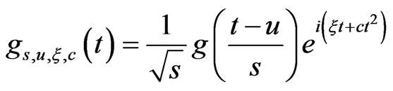
Equation (5) shows that the frequency of a Gabor atom keeps unchangeable as time changes, and it is not suitable for guided waves signal processing because guided wave’s propagation speed is changeable with different frequency. In this work, Chirplet functions [16] is selected as the matching atoms, and which can be expressed as
 (6)
(6)
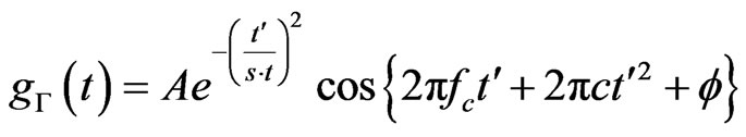
Since the detected signal is real valued, the real form of a Chirplet atom can be used as:
 (7)
(7)
The atom is specified by a set of parameters  associated with the signal characteristics. In which,
  ,
,  is the time,
  is the time delay determined by the distance of the reflection pulse echo signal from the exciting sensor and the defect or pipe end,
  is the central frequency of the exciting sensor,
  is the time spread with
  a non-dimensional parameter and
 ,
,  is the chirp-rate which reveals the signal frequency-varying behavior,
  is phase shift, and A is an arbitrary constant to satisfy
 .
.
Compared with Gabor atom, this model has an additional parameter, the chirp-rate c. Actually, Gabor atom is a special case of Chirplet atom with . The characteristics of the waveforms and Wigner distributions of Chirplet atoms with different chirp-rates are shown in Figures 1-3. In which, the time-frequency localization is excellent and different chirp-rates result in different slopes of the time-frequency distributions. Once the guided wave signal is decomposed into Chirplet atoms, the chirp-rate parameter will reflect the time-frequency character, so that the guided wave mode information is manifested [16].
3. Experiment Set-Up and Pipe Testing
3.1. Experiment Set-Up
A schematic diagram of the experimental set-up is shown
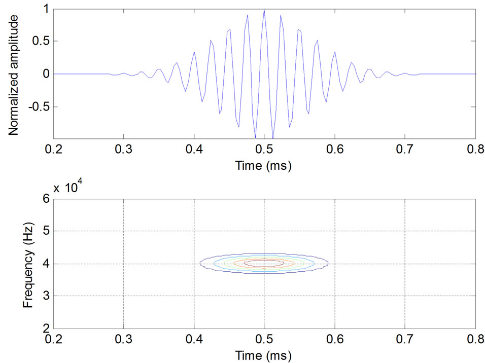
Figure 1. Waveforms and Wigner distributions of Chirplet atoms with c = 0.
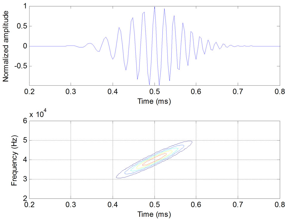
Figure 2. Waveforms and Wigner distributions of Chirplet atoms with c = 0.
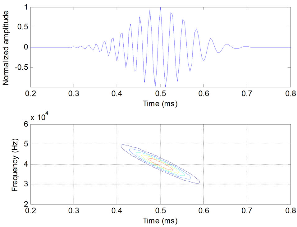
Figure 3. Waveforms and Wigner distributions of Chirplet atoms with c = 0.
in Figure 4. The set-up generates and detects elastic guided wave in steel pipe. A short-duration pulse of electric current generated from the signal generator and the signal is amplified by the power amplifier to load on the transmitting transducer. The magnet coil provides a DC bias magnetic field to the steel pipe. The elastic wave will be excited by the magnetostrictive effect. The elastic wave will propagate along the pipe axial direction and it will reflect to the receiving transducer when it arrive at the pipe end or defect. The receiving transducer detects changes in the magnetic induction of the pipe caused by the elastic wave via the inverse magnetostrictive effect. The received signal is amplified and processed by the filter and A/D convert circuit. The digital signal is transmitted to the collection circuit and displayed on the display. The defect can be found by analysis the detected guided wave signal.
3.2. Pipe Testing
Experiments are carried out to test the stainless steel pipe, and the laboratorial setup is described in Ref [19]. Two stainless steel pipes with length of 6.4 m, outer diameter of 56 mm and wall thickness of 3 mm are used in the experiment. One pipe has no defect and another pipe has a hole with diameter of 10 mm and depth of 2 mm, as shown in Figure 5.
The dispersion curves of the guided waves in the pipe are illustrated in Figures 6 and 7. There are three different modes at any frequency, and the character of each mode is unique. “L” represents the longitudinal modes, “T” represents the torsional modes and “F” represents the flexural modes.
It is easy to found that the T(0, 1) guided wave is non dispersion, therefore the no defect steel pipe is tested by 62 kHz T(0, 1) guided wave and the defect pipe is tested by 26 kHz T(0, 1) guided wave, respectively.
4. Guided Waves Mode Discrimination Based on MP
In this section, the detected signals are processed and the guided wave modes will be identified by MP.
4.1. Guided Waves Mode Discrimination on Integrated Pipe NDT Signal Based on MP
The detected signal for the no defect steel pipe by 62 kHz T(0, 1) guided wave is shown in Figure 8. Except that T(0, 1) mode represents reflections from the pipe end, there are also reflections of two unknown modes, tagged as mode 1 and mode 2, respectively. Concentrated on signals within the dashed line domain in Figure 8, the processed result by matching pursuit method is shown in Figure 9.
Three reflections of different modes are extracted and
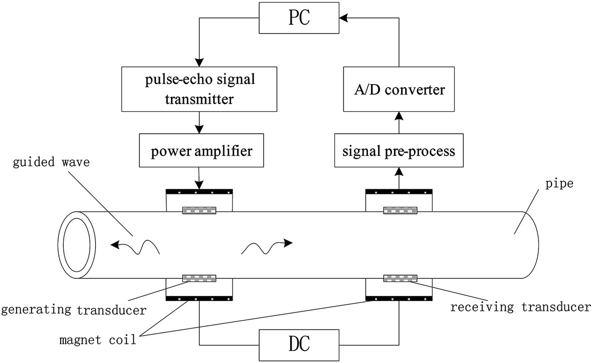
Figure 4. The experimental set-up schematic diagram.
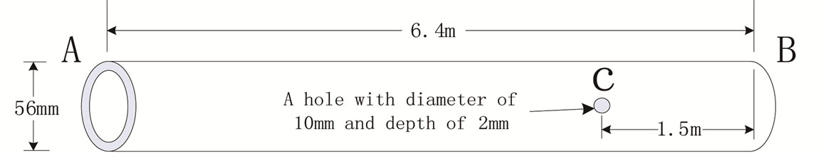
Figure 5. The stainless steel sample pipe.
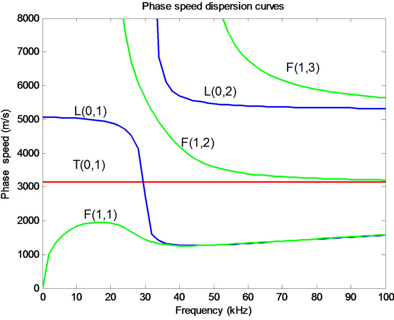
Figure 6. Phase velocity dispersion curves of stainless steel pipe with outer diameter of 56 mm.
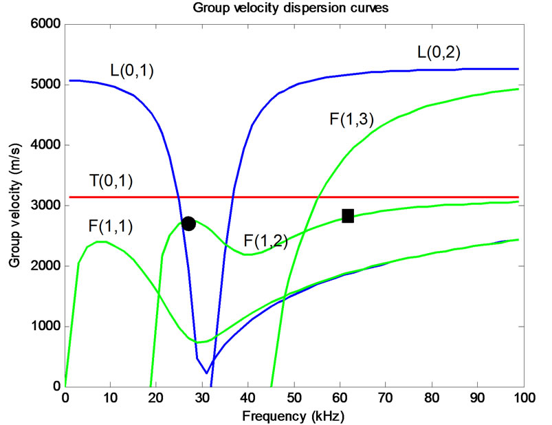
Figure 7. Group velocity dispersion curves of stainless steel pipe with outer diameter of 56 mm.
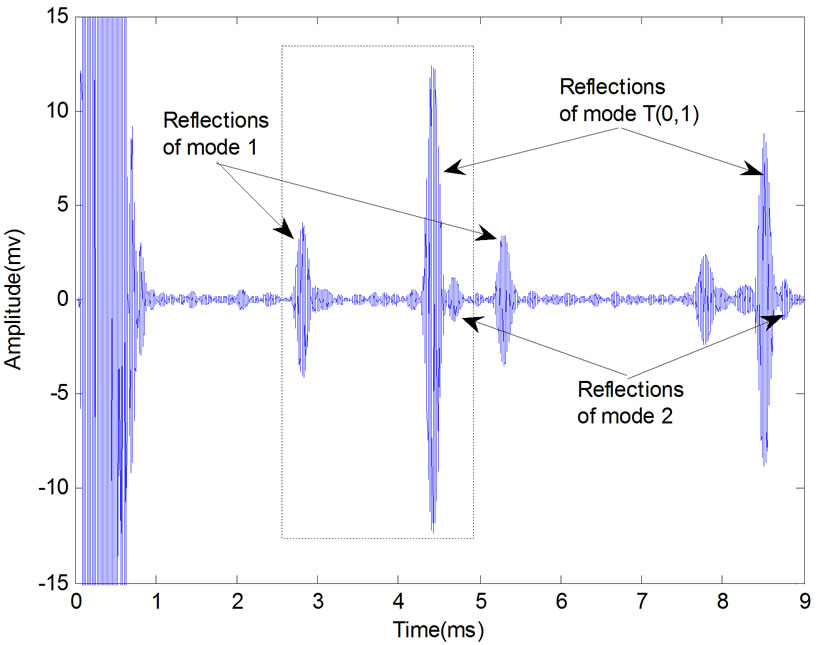
Figure 8. Detected signal of no defect stainless steel pipe.
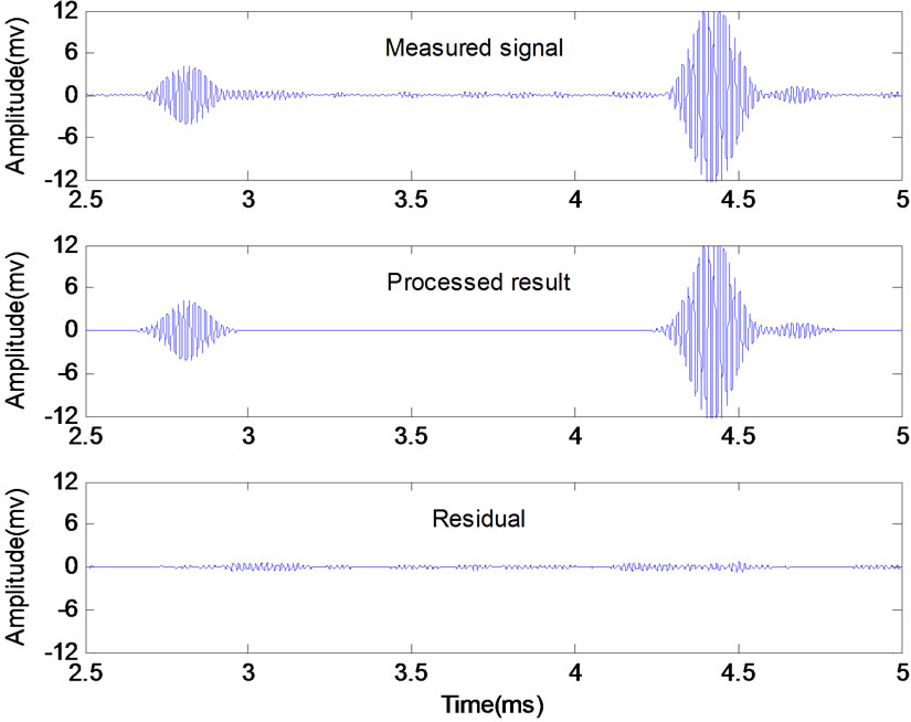
Figure 9. The intercepted signal processed by matching pursuit.
their Chirplet atoms’ parameters are shown in Table 1. Results in this table reveal information of each reflection, such as the center frequency, arrival time, time spread, chirp-rate and amplitude.
According to Table 1, the value of parameter chirprate c is a small negative value for the reflection of T(0, 1) mode, and which agrees with the non-dispersion character of T(0, 1) mode. But the values of parameter c are bigger negative value for the two unknown modes, and the value of  and amplitude of the two unknown modes is smaller than that of T(0, 1) mode, which indicates the two unknown modes can be divided from T(0, 1) mode.
Superimposing the Wigner distributions of the atoms decomposed in the time-frequency plane, we can get the time-frequency representations without interference terms as shown in Figure 10. Contour plot of the attained TFRs with the group velocity dispersion curves is shown in Figure 11.
In Figures 10 and 11, the TFRs of each echo reveal their time-frequency character and matches excellently with the dispersion curves. By comparison, it is easy to identify mode 1 is the L(0, 2) longitudinal mode. But the mode 2 doesn’t overlap with any group velocity curves, which means that it is not excited by the emitting sensor. From Figure 11, the mode 2 is located between the curves of T(0, 1) and F(1, 2), therefore it can be concluded that the mode 2 is the converted mode by T(0, 1) at the the right end of pipe, and the mode is converted into F(1, 2).
To verify the above conclusions, further numerical calculation is performed. For the sample steel pipe, the group velocity of mode T(0, 1) is 3138 m/s, but the group velocity of the mode 2 is 2787 m/s. This velocity agrees with the group velocity of mode F(1, 2) at 62 kHz, which is highlighted by a square mark in Figure 7, so that the mode 2 is confirmed as the mode F(1, 2).
4.2. Guided Waves Mode Discrimination on Defect Pipe NDT Signal Based on MP
The detected signal for the defect steel pipe by 26 kHz T(0, 1) guided wave is shown in Figure 12. The signal include defect echo is processed by MP and the result is shown in Figure 13.
Figure 12 shows the defect echo consists of two wave-packets which is illustrated in Figure 13, tagged wave-packet 1 and wave-packet 2, respectively. The Chirplet atoms’ parameters of the two wave-packets decomposed are shown in Table 2. Interference free TFRs of constituent Chirplet atoms for the wave-packets is shown in Figure 14, and the contour plot with the group velocity dispersion curves of the TFRs is shown in Figure 15.
By comparing and analyzing the chirp-rate values, we can obtain that the two wave-packets belong to different modes. Figure 14 shows that wave-packet 1 is the defect echo of mode T(0, 1) and the wave-packet 2 is generated by mode conversion at the defect.
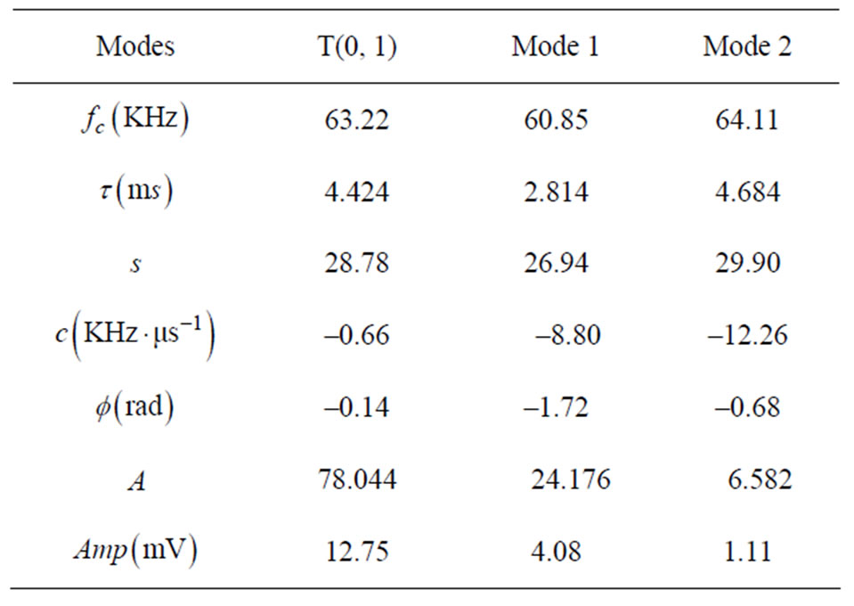
Table 1. Chirplet atom parameters of the processed signal.
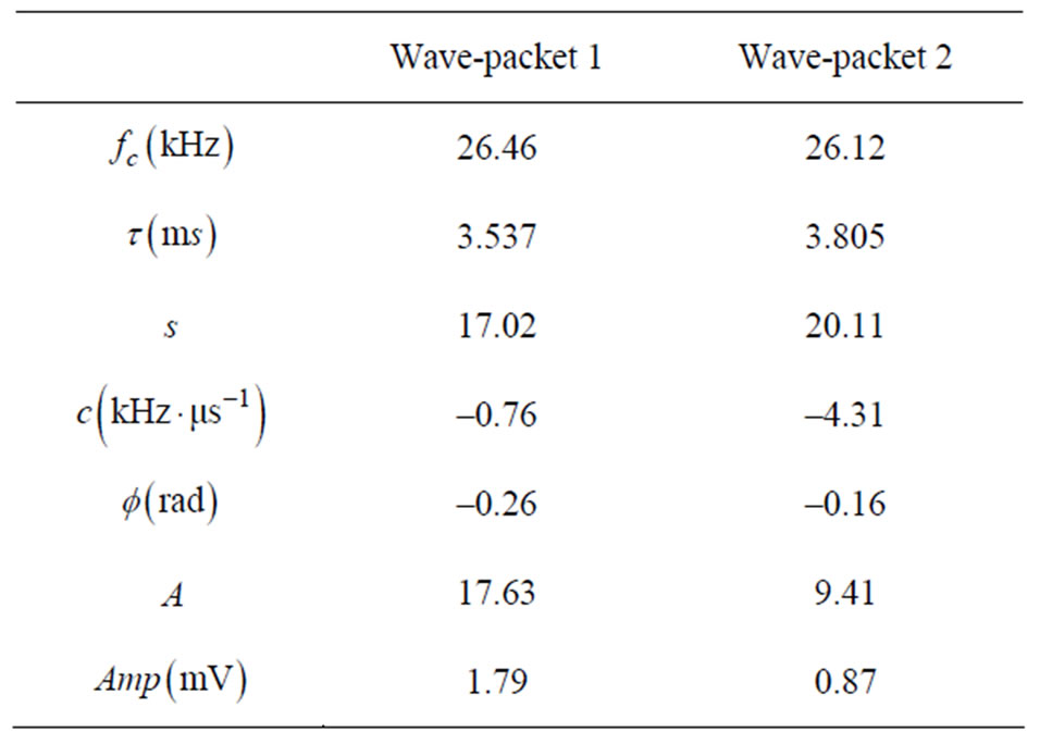
Table 2. Chirplet atom parameters for the two wavepackets.
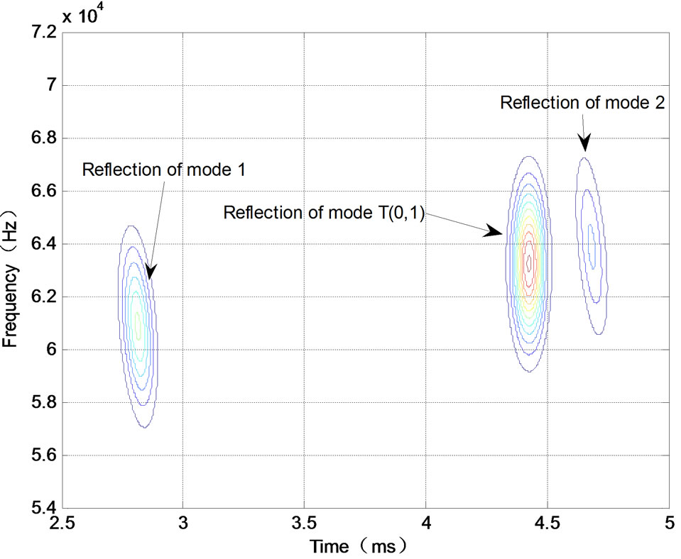
Figure 10. The achieved interference free TFRs.
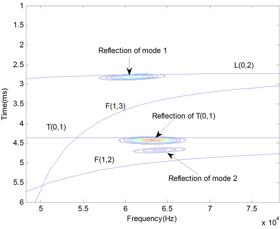
Figure 11. Comparison between the TFRs and dispersion curves.
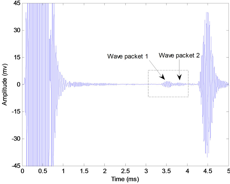
Figure 12. Detected signal of the defect stainless steel pipe.
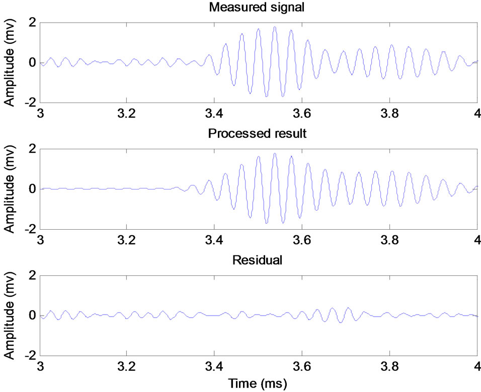
Figure 13. The intercepted signal processed by matching pursuit.
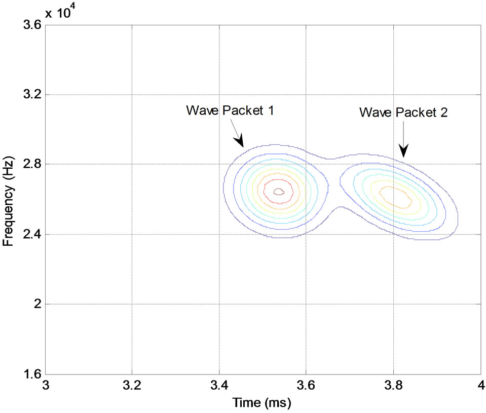
Figure 14. TFRs of the two waveforms.
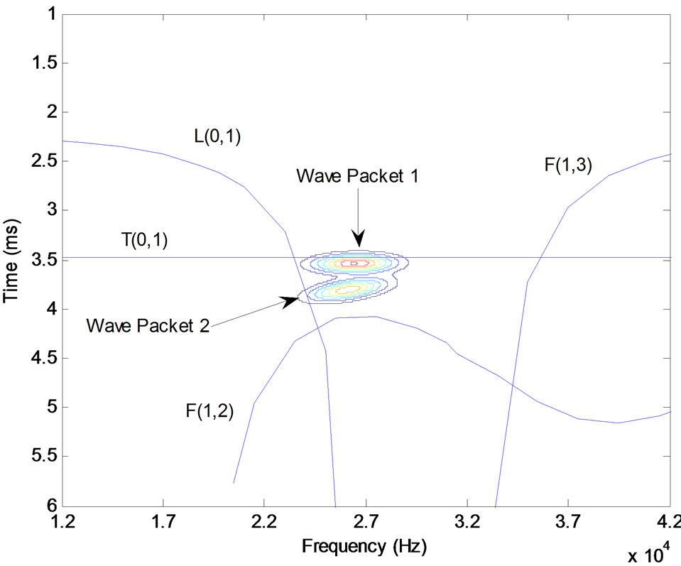
Figure 15. Comparison between the TFRs and dispersion curves.
Similarly, the velocity of wave-packet 2 with parameters ,
, (arrival time of the two wave-packets) and
  (velocity of T(0, 1) mode) is
 . This value is close to the velocity of mode L(0, 1) and mode F(1, 2) at 26 kHz as highlighted by a circular mark in Figure 7. It is undistinguishable that the wave-packet 2 belongs to which mode from amount of velocity merely. Because the value of chirprate c of the wave-packet 2 is bigger negative value, and the group velocity of the wave-packet 2 ascends with the increase in frequency, which agrees only with the character of mode F(1, 2), the conclusion that the wave-packet 2 belongs to mode F(1, 2) can be deduced. This conclusion holds true in the general phenomenon, viz. the axisymmetric modes are converted to the non-axisymmetric modes, when guided waves encounter the defect in pipes.
5. Conclusion
The Chirplet matching pursuit can extract the guided waves echo signal, and the results shows some information of guided waves such as the signals center frequency, arrival time, time spread and frequency-varying characteristics, which are affected by ultrasonic guided waves echo mode. In the experiment, ultrasonic guided waves technology is used to detect two kinds of stainless steel pipes, one pipe has no defect and another pipe has a hole defect. For the pipe with no defect detection, the detected guided waves mode with T(0, 1), F(1, 2) and L(0, 2) are respectively identified. For the pipe with defect detection, the defect reflection signals consisted of two wavepackets with T(0, 1) and F(1, 2) mode are also identified. It is shown that the matching pursuit method has a tremendous advantage to identify different guided waves modes signals in pipes non-destructive testing.
REFERENCES
- F. C. He, Y. F. Gao, Z. G. Zhou, et al., “An Overview of Testing Application of Wavelet in Guided Waves,” 12th Asia-Pacific Conference on Non-Destructive Testing, Auckland, 2006.
- D. Alleyne and P. Cawley, “A Two-Dimensional Fourier Transform Method for the Measurement of Propagating Multimode Signals,” Journal of the Acoustical Society of America, Vol. 89, No. 3, 1991, pp. 1159-1168. doi:10.1121/1.400530
- Y. X. Sun, B. Wu and C. F. He, “Application of TimeFrequency Analysis in Propagation Characteristic of Guided Waves in Rod,” Chinese Journal of Scientific Instrument, Vol. 27, No. 6, 2006, pp. 1315-1317.
- W. W. Zhang, Z. H. Wang and H. W. Ma, “Correlation Analysis of Ultrasonic Guided Wave in Damaged Pipe,” Journal of Jinan University, Natural Science, Vol. 30, No. 3, 2009, pp. 269-272.
- J. Zou, X. J. WU, J. Xu, et al., “Identification of Magnetostrictive Guided Wave Signal Based on Duffing Chaotic Oscillators,” Nondestructive Testing, Vol. 30, No. 9, 2008, pp. 600-603.
- S. G. Mallat and Z. F. Zhang, “Matching Pursuit with Time-Frequency Dictionaries,” IEEE Transaction on Signal Processing, Vol. 41, No. 2, 1993, pp. 3397-3414. doi:10.1109/78.258082
- N. Ruiz-Reyes, P. Vera-Candeas and J. Curpian-Aloma, “Matching Pursuit-Based Approach for Ultrasonic Flaw Detection,” Signal Processing, Vol. 86, No. 5, 2006, pp. 962-970. doi:10.1016/j.sigpro.2005.07.019
- D. W. Wang, X. Y. Ma, X. P. Guan, et al., “Matching Pursuits Based Feature Extraction with Reduced Aspect Sensitivity for Ultra Wide-Band Radar Target Identification,” CIE International Conference on Radar, Beijing, 2006, pp. 1-4.
- S. B. Kim, A. Chattopadhyaya and A. D. Nguyen, “The Use of Matching Pursuit Decomposition for Damage Detection and Localization in Complex Structures,” Proceeding of SPIE, Vol. 7981, No. 29, 2011, pp. 1-9.
- A. Papandreou-Suppappola and S. B. Suppappola, “Analysis and Classification of Time-Varying Signals with Multiple-Frequency Structures,” IEEE Signal Processing Letters, Vol. 9, No. 3, 2002, pp. 92-95. doi:10.1109/97.995826
- R. Mazhar, P. D. Gader and J. N. Wilson, “A Matching Pursuits Based Similarity Measure for Fuzzy Clustering and Classification of Signals,” IEEE International Conference on Fuzzy Systems, Hong Kong, 1-6 June 2008, pp. 1-4.
- N. Ruiz-Reyes, P. Vera-Candeas and J. Curpian-Aloma, “High Resolution Pursuit for Detecting Flaw Echoed Close to the Material Surface in Ultrasonic NDT,” NDT&E International, Vol. 9, No. 39, 2006, pp. 487-492. doi:10.1016/j.ndteint.2006.02.002
- S. Jaggi, W. C. Karl and S. Mallat, “High Resolution Pursuit for Feature Extraction,” Applied and Computational Harmonic Analysis, Vol. 5, No. 4, 1998, pp. 428- 449. doi:10.1006/acha.1997.0239
- C. G. Benar, T. Papadoulo, B. Torresani, et al., “Consensus Matching Pursuit for Multi-Trial EEG Signals,” Journal of Neuroscience Methods, Vol. 180, No. 1, 2009, pp. 161-170. doi:10.1016/j.jneumeth.2009.03.005
- P. Xu and D. Z. Yao, “Two Dictionaries Matching Pursuit for Sparse Decomposition of Signals,” Signal Processing, Vol. 86, No. 11, 2006, pp. 3472-3480. doi:10.1016/j.sigpro.2006.05.006
- J. C. Hong, K. H. Sun and Y. Y. Kim, “The Matching Pursuit Approach Based on the Modulated Gaussian Pulse for Efficient Guided-Wave Damage Inspection,” Smart Structures and Materials, Vol. 14, No. 4, 2005, pp. 548-565. doi:10.1088/0964-1726/14/4/013
- A. Raghavan and C. E. S. Cesnik, “Guided-Wave Signal Processing Using Chirplet Matching Pursuit and Mode Correlation for Structural Health Monitoring,” Smart Materials and Structures, Vol. 16, No. 2, 2007, pp. 355-366. doi:10.1088/0964-1726/16/2/014
- F. C. Li, G. Meng, L. Ye, et al., “Dispersion Analysis of Lamb Waves and Damage Detection for Aluminum Structures Using Ridge in the Time-Scale Domain,” Measurement Science and Technology, Vol. 20, No. 9, 2009, pp. 1-10. doi:10.1088/0957-0233/20/9/095704
- Y. M. Wang, Y. H. Kang and X. J. Wu, “Application of STFT and HOS to Analyse Magnetostrictively Generated Pulse-Echo Signals of a Steel Pipe Defect,” NDT&E International, Vol. 39, No. 4, 2006, pp. 289-292. doi:10.1016/j.ndteint.2005.08.007
NOTES
*Corresponding author.