Int'l J. of Communications, Network and System Sciences
Vol.2 No.1(2009), Article ID:180,14 pages DOI:10.4236/ijcns.2009.21004
A Priority Queuing Model for HCF Controlled Channel Access (HCCA) in Wireless LANs
1Keylab of Information Coding and Transmission, Institute of Mobile Communications,
Southwest Jiaotong University, Chengdu, China
2Department of Computer Science, Georgia State University, Atlanta, GA, USA
Emails: r_ghazizadeh@yahoo.com, p.fan@ieee.org, pan@cs.gsu.edu
Received June 15, 2008; revised December 22, 2008; accepted December 31, 2008
Keywords: QoS, HCCA, Priority Queues, Matrix-Geometric Method, MAP/PH/1
Abstract
Recently, there has been a rapid growing interest in new applications requiring quality of service (QoS) guarantees through wireless local area networks (WLAN). These demands have led to the introduction of new 802.11 standard series to enhance access medium supporting QoS for multimedia applications. However, some applications such as variable bit rate (VBR) traffic address some challenges in the hybrid coordination function (HCF) nominated to provide QoS. This paper presents a novel priority queuing model to analyze a medium access in the HCF controlled channel access (HCCA) mode. This model makes use of a MAP (Markovian Arrival Process)/PH (Phase Type)/1 queue with two types of jobs which are suitable to support VBR traffic. Using a MAP for traffic arrival process and PH distribution for service process, the inclusion of vacation period makes our analysis very general and comprehensive to support various types of practical traffic streams. The proposed priority queuing model is very useful to evaluate and enhance the performance of the scheduler and the admission controller in the HCCA mechanism.
1. Introduction
Increasing demands to access to network in hotspots areas at airports, hotels, coffee shops have led wireless local area network (WLAN) to be a key technology for high-speed local access in public and private areas. Furthermore, in the near future, WLAN will play a key role within the hybrid wireless systems and also it is the best candidate to connect home devices to wireless networks. Therefore, it should be able to allow users to ubiquitously access a large variety of services. On the other hand, demands for new applications such as real time traffic, multimedia video and voice over IP are increasing rapidly. These applications have created need for QoS support.
However, IEEE802.11 is unsuitable for multimedia applications to support QoS in the MAC layer. Therefore, IEEE802.11 working group has been developing a new protocol, IEEE802.11e, which will be able to provide QoS features. IEEE802.11e introduces the hybrid co-ordination function comprised of two medium access mechanisms: contention-based channel access referred to as enhanced distributed channel access (EDCA) and controlled channel access referred to as HCF controlled channel access (HCCA) [1].
Although contention-based channel access is very simple and robust for best effort traffic, it can not provide QoS guarantees easily. These can be achieved with the polling-based medium access through the HCCA. The HCCA provides a hybrid coordinator (HC) with ability to assign a contention free time interval during contention period and contention free period to packet transmission. Therefore, transmission opportunity (TXOP) and service interval (SI) are very important parameters to provide QoS guarantees. A reference scheduler calculates these parameters with the reservation information achieved through the negotiation with the end users. Using average values, such as average packet length and average data rate, to compute transmission parameters cause some challenges to QoS support in VBR traffic. Therefore, modification of the scheduler to provide such traffic is very crucial. In this way, analytical system analysis is very useful to improve and develop the system.
This paper presents a priority queuing model to analyze a medium access in the HCCA. According to the HCCA characteristics, the model is based on a MAP/ PH/1 queue with vacation and time-limited service in the presence of two priority levels. Some important per-formance measures are presented after solving the queuing model through the matrix-analytic method [2,3]. To our best knowledge, although there are some papers which have investigated the HCCA and the EDCA through simulation [4-9], and the EDCA analytically [10-12], there is only one published analytical work for the HCCA [13], where a queuing model without priority levels has been developed. However, priority is a key point to separate various traffic streams with different QoS requirements, especially for real-time and non-real-time traffic. In addition, to manage resources, use bandwidth efficiently and provide QoS for various traffic streams, it is necessary that different traffic streams appear in the different statistic or dynamic priority levels in the system. Therefore, IEEE802.11e introduces four priority levels for eight groups of traffic streams. Consequently, to modify and investigate the performance of the scheduler and the admission controller, priority analytical model in the presence of prioritized traffic is very helpful. In [14], a priority model in a medium without a vacation period and time-limited service was introduced. That model can not be applied to the HCCA medium access which is based on a vacation period and time-limited service. This paper will present a priority queuing model to analyze medium access in the HCCA by making use of an MAP/PH/1 queue with two types of jobs which are suitable to support vast practical traffic streams.
The rest of the paper is organized as follows: in Section 2, we briefly describe the HCCA mechanism, phase type (PH) distribution and discrete Markovian arrival process (DMAP); our proposed model is presented in Section 3; the related performance measures are analyzed in Section 4; numerical and simulation results are given in Section 5; and finally conclusions are drawn in Section 6.
2. HCCA and System Parameters
2.1. HCCA
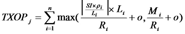
IEEE802.11e/HCCA is a polling-based medium and centralized scheduling which is controlled by the HC. Each station that requires a strict QoS support is allowed to send QoS requirement packets to the HC and the HC assign a corresponding transmission opportunity to the station. The HC can start a polling period at any time during a contention period after the medium remains idle for at least point coordination function (PCF) inter-frame space interval. Each station can transmit a sequences of data packets separated by a short inter-frame space during own TXOP allocated by the HC in a contention free period. Therefore, as it has shown in Figure 1, a sequence of transmission opportunities will be assigned to the stations during each SI. Consequently, each station is polled once per SI and allowed to transmit its packets until its TXOP duration elapses. Uplink and downlink TXOPs are initiated by the scheduler in the HC and end when there is no packet in the queues for transmission or TXOP duration expires. To provide QoS, each station manages QoS control field added to the legacy frames. Consequently, the scheduler receives separated reservation information of different traffic streams to calculate an aggregated service schedule. Some of this information is the mean data rate, delay bound, maximum burst size, minimum physical rate, user priority and peak data rate. The scheduler, first of all calculates the maximum service interval according to the delay bound for each traffic stream. Then, it selects the smallest service interval among all the maximum service intervals corresponding with the traffic streams as a service interval for all stations. The scheduler after that determines TXOP for each traffic stream according to the negotiated reservation information. Allocated TXOP for each station is sum of all TXOPs of station’s traffic streams. TXOP of jth station that has made n traffic streams is computed as follows.
 (1)
(1)
where R denotes the minimum physical data rate, L and M represents the nominal and the maximum size of packet respectively,  denotes the mean data rate and O represents the overhead due to the physical and MAC headers, acknowledgment and polling frames. According to the service interval duration, the number of active stations and the TXOP duration in each station, an admission controller manages the number of active stations to provide QoS.
2.2. Discrete Markovian Arrival Process (DMAP)
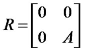
Consider a discrete time Markov chain with a transition matrix D and two sub-stochastic matrix , where
 . Suppose at the time t, the Markov chain is in the state
 . Then, at the time epoch t+1 with probability
  arrival process enters state
  and starts a batch of k arrivals. Therefore,
  corresponds to a transition matrix with no arrival and
  corresponds to a transition matrix with only one arrival per time slot.
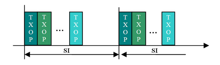
Figure 1. TXOP allocation in contention free period.
2.3. Phase Type (PH) Distribution
Phase type distributions can approximate many of general distributions encountered in queuing systems. Therefore, it is appropriate in service time modeling [2]. Consider an m+1 states Markov chain with one absorbing state, and initial probability vector  with m+1 elements where
  is a row vector with m element while
  (
( is column vector of one). Let the transition probability matrix of the Markov chain be P:
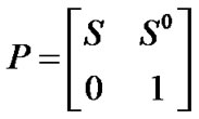 .
.
where S is a sub-stochastic transition matrix, I-S is nonsingular (I is identity matrix) and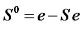 . The absorbing Markov chain can initialize from any states according to the initial vector and gets absorbed to the absorbing state. Therefore, the time to absorption in such a Markov chain is said to have phase type distribution which is represented with the pair
 .
.
3. Proposed Priority Queuing Model
To clarify the model, suppose that there is one station communicating with the HC in the system. The HC can be considered as a single server which serves queues (high and low priority) of the station no more than T slots (maximum TXOP duration is divided to T slots) during each SI. In the view of the station, as soon as T time slots is used up or queues become empty, the server goes on a vacation (i.e. the server serves other stations or becomes idle until the next visit). Hence, as it is illustrated in Figure 2, the minimum vacation duration is subtraction of the SI and the maximum TXOP duration. It is assumed that the HC is a server which serves priority queues in non-preemptive priority case during a TXOP period. In a non-preemptive case, no service interruption is applied upon arrival of a high priority packet when a low priority packet is being served. To analyze the discrete time Markov chain (DTMC) describing the queuing model, arrival process, service process and vacation model are defined. The arrival process is modeled by a discrete Markovian arrival process (DMAP) to allow correlation among the inter-arrival times within packets (within each priority and between two priorities packets) and support various types of traffic streams, especially VBR traffic which generate packets in random arrival intervals. On the other
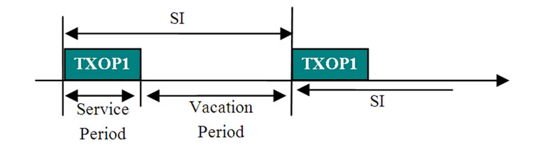
Figure 2. Service and vacation periods for one station in HCCA.
hand, it is obvious that the packet transmission time is corresponding to the service time which depends on the packet length while the channel data rate is fixed. Therefore, to support various packet length distributions and make the model of service process more general and comprehensive, a phase type (PH) distribution is proposed for a service process model. Consequently, the introduced priority queuing model is based on a MAP/ PH/1 queue with vacation and time-limited service. The proposed model is based on the work of [14] which makes use of matrix-geometric solution for analysis priority queues without vacation and time limitation in service.
Some of the notations and symbols which will be used throughout the paper are introduced as follows:  is a column vector of one (with appropriate order equals to the number of columns of the matrix or to the vector length that it is multiplied with),
  represents a column vector of zeroes with T length except at the vth position that is one,
 ![]() is the transpose of
is the transpose of  vector,
  denotes an identity matrix of dimension
  and
and  represents
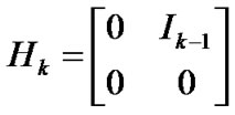 .
.
3.1. Arrival Process
The arrival process is modeled by a discrete Markovian arrival process (DMAP). The DMAP, an extension of the Markov modulated Bernoulli process, can support many types of traffic flows such as VBR traffic generating variable packets length in variable inter-arrival periods. Suppose there are two independent types of traffic corresponding to two priorities where each traffic source is able to generate only one packet per time slot. Hence, each traffic flow will have two sub-stochastic matrices(Section 2.2) and consequently there are four sub-stochastic matrixes (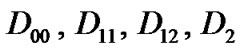 ) corresponding to join packet arrival (high priority and low priority packet arrival) where
  denotes a transition matrix with no packet arrival,
  is a transition matrix when one high priority packet arrives,
  represents a transition matrix when one low priority packet arrives,
  is a transition matrix when two high and low priority packet arrive(one of each priority packet) and also
 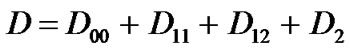 where
where represents stochastic matrix. The arrival rate is
 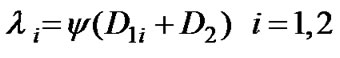 where
where  and
and  (e is a column vector of one).
As mentioned above, four sub-stochastic matrices can be expressed by the sub-stochastic matrices of both traffic streams. Suppose  and
and  are the transition matrices in the high priority traffic when no packet and one packet arrives at a time slot, respectively. Furthermore assume,
  and
and  are the transition matrices in the low priority traffic when no packet and one packet arrives at the time slot respectively. In this case,
 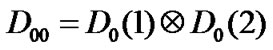 ,
, 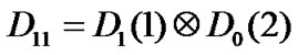 ,
, 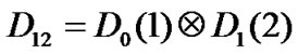 and
and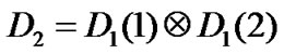 , where
  is the Kronecker product.
3.2. Service Process
The service process is corresponding to the transmission time. The total transmission time of a frame is sum of transmission time of data packet, its necessary headers added by the MAC and physical layer, ACK, and short inter-frame space (SIFS). We assume that the channel data rate, ACK, SIFS durations and header size are fixed. Hence, the service time of a packet can be considered as a random variable which varies only with the length of the packet. Consequently, to generalize the model and support different packet length distributions, we consider phase type distribution for both high priority and low priority service processes. Let  and
and  denote PH distribution for high priority and low priority services, respectively where
  are transition matrices of dimensions
 , respectively and
  represent initial vectors.
 ,
, 
 are transition to absorption vectors for the high priority and low priority services, respectively.
3.3. Vacation Model
In the service period, whenever there is no packet in the queues or the TXOP duration expires, the server enters a vacation period. Therefore, the vacation duration depends on the service duration. A vacation with the maximum duration begins whenever the server visits the station at the first slot of TXOP and the station has no packet to transmit. Consequently, a vacation model can be represented by a  phase type distribution while the Markov chain can initialize from any states depending on the vacation duration. Therefore, the initial vector, the transition matrix and the transition to absorption vector will be
 ,
,  and
and 
 , respectively.
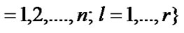
3.4. State Space and Transition Matrix of the DTMC
In this subsection, we introduce state space and the transition matrix of the discrete time Markov chain (DTMC). The state space can be divided into two main groups that are vacation and service state spaces. Each of these states are described by the number of the packets in the high priority and low priority queues (i1,i2), the phase of the arrival process (j), the phase of the high priority or low priority service processes (k1,k2), the phase of the vacation  and the phase of the TXOP
 . Therefore, the states can be expressed as follows.
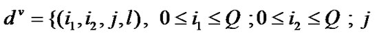

 (2)
(2)

where Q is the buffer size in the number of packets (high priority and low priority),  denotes the vacation states while the number of high priority and low priority packets in the queues are i1 and i2 respectively and the packet arrival is in j th phase as well as vacation is in
  th phase,
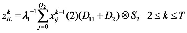
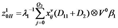
  represents service state space when there are only low priority packets in the system. Therefore, a low priority packet is being served while the service is in the phase K2 at
  th time slot and the packet arrival is in j th phase as well. In the same way,
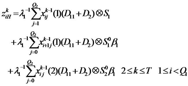
  is service state space when there is at least one high priority packet in the system and a low priority packet is being served, and
  represents service state space when there is at least one high priority packet in the system and a high priority packet is being served.
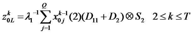
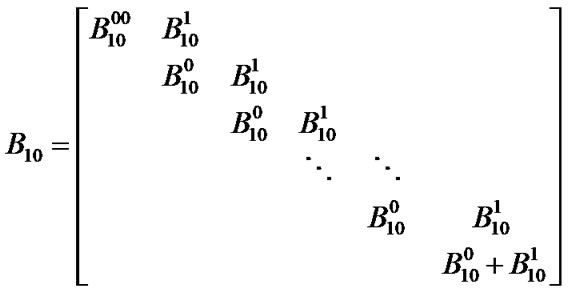
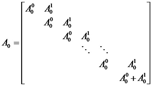
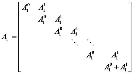
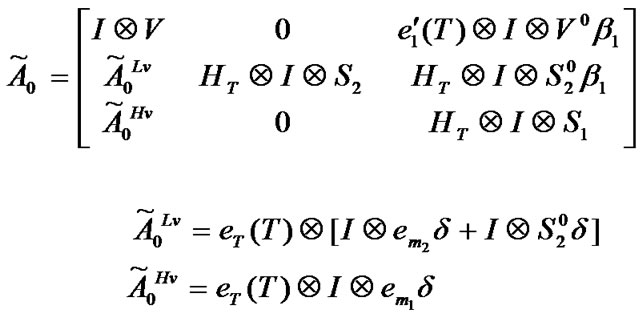
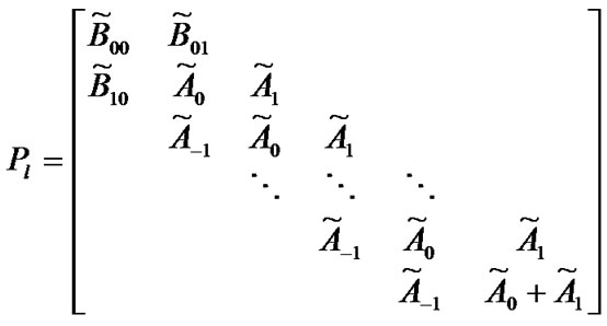
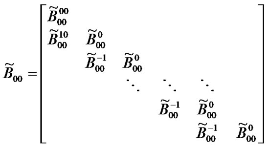
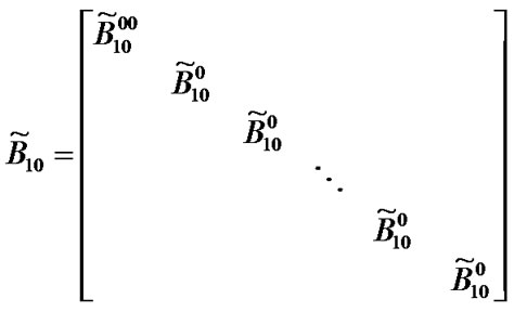
The transition matrix of the discrete time Markov chain can be expressed as follows.
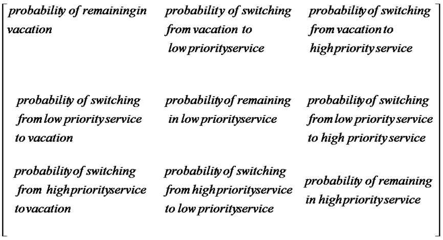
Figure 3. General form of the transition probability sub matrix.
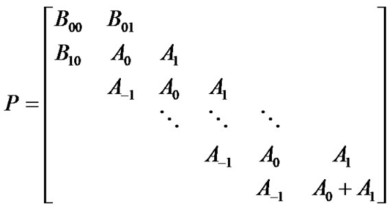 (3)
(3)
where the rows of P matrix correspond to the number of packets in the high priority queue. Therefore, matrix will have  rows. As it is assumed that each type of traffic can generate only one packet and only one packet can be served per time slot (less than or equal to one), the structure of P matrix is quasi-birth-death. Consequently, the elements of matrix P represent block transition matrices in which the number of packets in the high priority queue increases (
 ) or decreases (
 ) by one, or remains invariant (
 ) after transition at the current time slot. On the other hand, each element of P matrix also represents one matrix describing low priority queue size. Therefore, each row of
 block matrices, described as follows, represents the number of low priority packets in the queue.
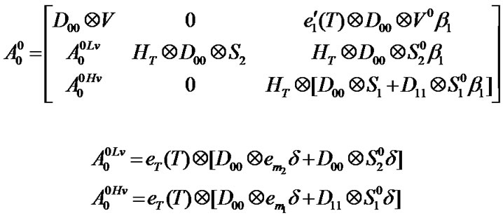
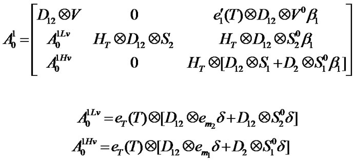
To describe each sub matrix (with general form  or
or ), a general sub matrix form is defined in Figure 3. The general sub matrix can be understood as the transitions probability matrix governing switch among a vacation, a high priority and a low priority service. Note that the maximum service duration is T slots and transition can happen at any time slots. Therefore, service period in the general matrix is divided to T slot (in high priority and low priority). It is obvious that some of the state transitions in the general matrix may not happen. Therefore, those states will be zero. To reduction of the matrix dimensions, those rows and columns of the general matrix which are zero will be removed if the general matrix can match with the other matrices in the P matrix. Now, in the rest of this sub section, we express the sub matrices by considering the possible state transitions in the general matrix form.
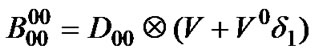
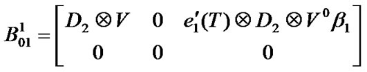
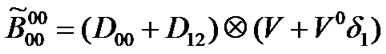
 (4)
(4)
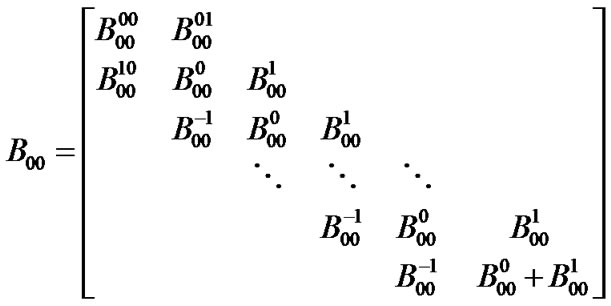
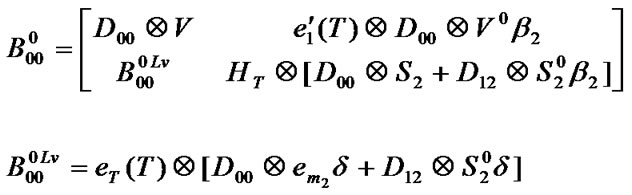
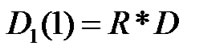
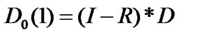
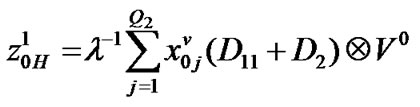
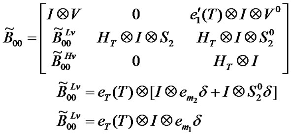
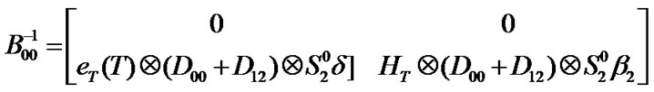
Block matrix  represents state transitions when high priority and low priority queues are empty and remain empty after transition. Transitions occur whenever no packet arrives (D00) and the server is on vacation (V), or completes vacation (V 0) and starts it again. As there is no packet to be served, the maximum vacation duration will be initialized (
 ).
).
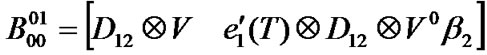
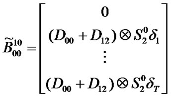
 (5)
(5)
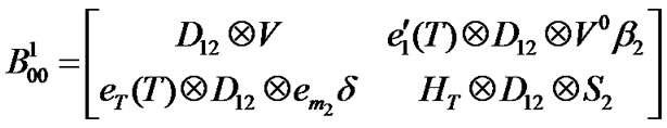
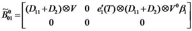
 matrix denotes transitions in which the number of packets in the low priority queue increases by one while the both queues are empty. Transitions occur whenever only a low priority packet arrives (D12) and the server stays on vacation (V) or completes vacation (V0) and starts the low priority service (
 ) at the first slot of the TXOP.
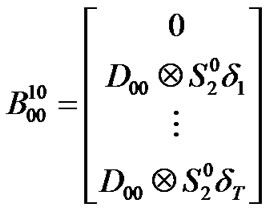
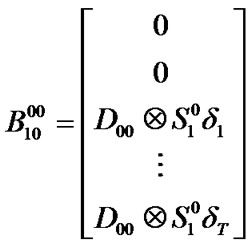
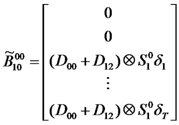
 (6)
(6)
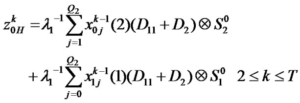
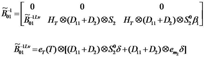
It is assumed that whenever the both queues become empty the server goes on vacation. The vacation can begin from different states of its Markov chain which is dependent on the instant that the queues become empty in the service period.  supports state transitions that no packet arrives (
 ), the process of the last low priority packet is completed. Consequently, queue become empty and the vacation period begins (transitions can happen at any time slots in the TXOP period) (
 ).
).
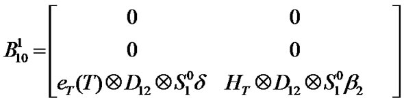
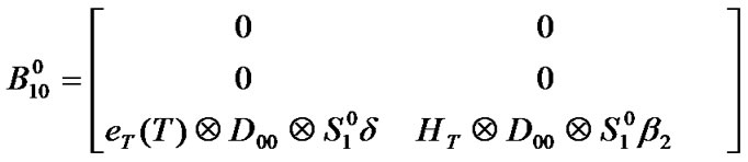
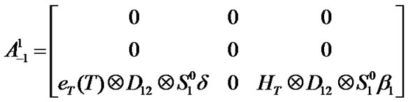
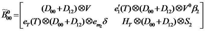
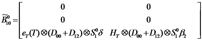
 (7)
(7)
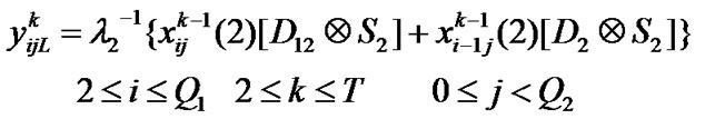
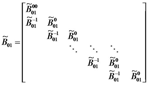
 block matrices represent transitions in which the number of packets in the low priority queue remains invariant, increases, decreases by one respectively while the high priority queue remains empty after transition, and there is at least one packet in the low priority queue before transition. These conditions can happen on the vacation, or in the service (low priority queue is served).
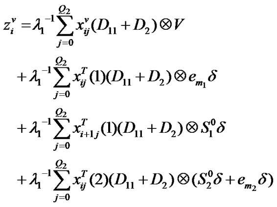
Now, we explain possible state transitions in the block matrix . We divide transitions into two cases. 1) no packet arrives (
 ), and a) the server remains on vacation (
 ), b) the server ends vacation and goes on the low priority service (
 ) at the first slot of TXOP (i.e.
 ). c) the server remains on the processing of low priority packet (
 ), d) the server leaves the service processing due to the TXOP expiration (
 ) and enters vacation(
 ). 2) a low priority packet arrives (
 ), and a) the processing of a low priority packet is completed and a new low priority processing begins (
 ), b) the processing of a low priority packet is completed while the TXOP duration expires as well and the server goes on vacation(
 )
)
 (8)
(8)
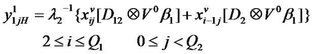
 contains the state transitions increasing the number of packets in the low priority queue by one and remaining the high priority queue empty while there is at least one packet in the low priority queue before transition. One can easily compute the possible transitions such above discussions
 (9)
(9)
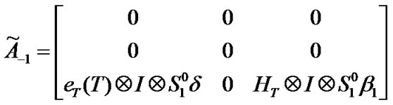
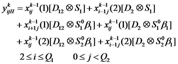
 represents state transitions in which the number of packets in the low priority queue decreases by one and at least one packet is in the low priority queue before transition as well as high priority queue remains empty. These transitions happen when no packet arrives and the processing of a low priority packet is completed, and a) the processing of another one begins, b) the TXOP duration expires and a vacation period begins.
 (10)
(10)
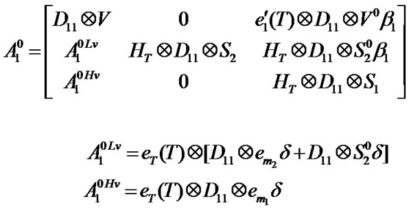
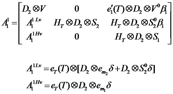
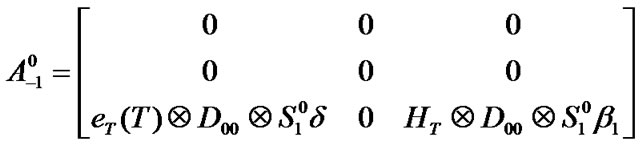
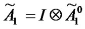
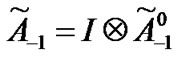
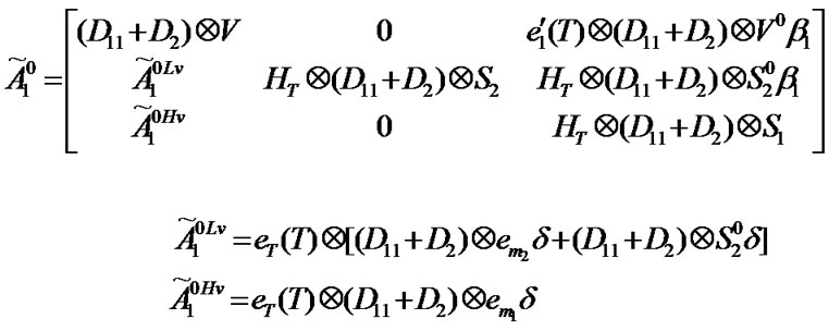
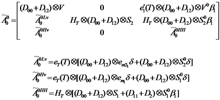
 and their elements can be computed in the same manner. The block matrices are given in Appendix A.
4. Performance Measures
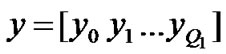
According to the structure of P matrix, its steady state distribution vector can be obtained by applying the matrix-geometric method. Let probability steady state distribution vector be x =[x0 x1 x2 … xQ] where xi =[x i0 x i1 x i2 … x iQ]xij=[ xij (1) xij(2)] and xij(k)=[
 …
… ]0≤i≤Q, 0≤j≤Q, k =1,2 where
  is the probability that the number of packets in the high priority and in the low priority queues are
  and
and  respectively while type
  packet (
 : high priority,
 : low priority) is being served at the
 ![]() th time slot of the TXOP period.
th time slot of the TXOP period.
Using balanced equations ( ( and the matrix-geometric method, the steady state vector
  can be calculated. For more details of how to find out steady state vector, readers can refer to [2].
4.1. Queue Length Distribution
Let  (
( ) be the probability that there are
  high priority packets (low priority packets) in the queue. The length of the high priority queue will be
  if there are
  high priority packets in the system and the server is not on the processing of the high priority packet (i.e. is on vacation or in the processing of the low priority packet) or,
  high priority packet are in the system while one high priority packet is being served.
 (11)
(11)
 (12)
(12)
Probability of the queue length at the end of the TXOP duration can be calculated in the similar manner.
4.2. Packet Loss Rate
Packet loss occurs whenever a new packet arrives and the target buffer is full. These conditions can happen during service processing (at any time slots of the TXOP duration) or vacation.
The high priority packet will be lost when the number of packets in the high priority queue is  (regardless of the number of packets in the low priority queue) and a new high priority packet arrives (by itself or together with a low priority packet) (
 ). Therefore, the packet loss probability will be sum of all possible probabilities among vacation and service period satisfying above conditions. As an example,
  shows sum of the probabilities in which the server stays on the high priority processing while a new high priority packet arrives and the other mentioned conditions has been satisfied. Consequently the high priority Packet loss rate which is normalized with the high priority arrival rate (
 ) is expressed as follow.
 (13)
(13)
At the same way, Packet loss in the low priority queue occurs when the low priority queue is full and a new low priority packet arrives ( ). Therefore all possible states satisfying those conditions could be expressed as follows.
 (14)
(14)
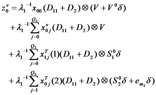
4.3. Access Delay Distribution
In this subsection, we introduce access delay distribution for the high priority and the low priority packets. Access delay is the required time in which an arriving packet at the target queue reaches the head of queue. Access delay can be studied as an absorbing Markov chain. The chain initializes when the packet arrives the queue, and gets absorbed when the packet reaches the head of the queue. Therefore, the access delay is the required time to absorption in the Markov chain.
In the high priority queue, experienced delay is the period of the time in which an arriving packet has to wait until all high priority packets ahead of it are served, and the process of a low priority packet, which is being processed at the arrival time, is completed Therefore, the access delay in the high priority queue depends on the number of the high priority packets ahead of an arriving packet. Suppose ![]() defines the initial probability vector in the high priority access delay.
defines the initial probability vector in the high priority access delay.
 (15)
(15)
where  and
and  denote the pro-bability of the arriving high priority packet finding i high priority packet ahead of it with the server: in vacation, in the low priority processing at the
 ![]() th slot of the TXOP and, in the high priority processing at the
th slot of the TXOP and, in the high priority processing at the ![]() th slot of the TXOP, respectively.
th slot of the TXOP, respectively.
Probability vector  represents the probability of arriving high priority packet (
 ) (regardless of low priority packet arrival), finding no high priority packet ahead of it with server: on vacation. The possible scenarios are a) there is no packet in the high priority queue and the server stays on vacation (
 ), b) the server completes the processing of the last high priority packet in the Tth slot (the last slot of TXOP) and goes on vacation, c) the server leaves the low priority processing due to the TXOP expiration and goes on vacation, d) the server completes the low priority processing at the Tth slot and goes on vacation. Consequently,
  which is normalized by
  can be expressed as follows.
 (16)
(16)
 represents the probability vector in which arriving high priority packet finding no high priority packet ahead of it while server is serving a low priority packet at the kth slot of the TXOP. It can occur when the server stays on the processing of a low priority packet at the kth slot of the TXOP while high priority packet arrives.
 (17)
(17)
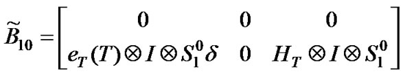
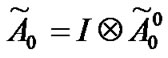
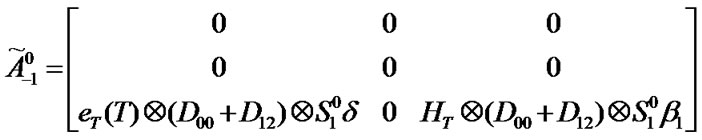
The other elements which are given in Appendix B can be calculated using similar above discussions Now, to find the time till absorption in a Markov chain, the transition matrix for high priority packet access delay ( ) is required. This matrix is defined as follows.
 (18)
(18)
It is obvious that the access delay for an arriving high priority packet only depends on the number of high priority packets ahead of the arriving packet. The number of packets which arrives after desired packet has no effect on the access delay. Therefore, the arrival transition matrix will be I. Now, each element of  matrix can be computed with the similar discussions in the Section 3.4. For example,
  represent state transitions when the number of packets ahead of arriving packet changes from 1 to 0 at the end of transition. It is obvious that transitions occur when the high priority processing is completed.
 (19)
(19)
The other elements are given in Appendix B. Finally, the probability vector after elapsing n+1 time slot will be
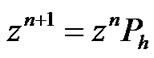 (20)
(20)
where . To reduction of computation, the set of following equation can be used.
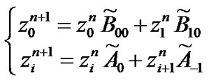 (21)
(21)
Finally, let  be the probability that the waiting time of high priority packet is less than or equal to T, then
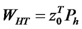 (22)
(22)
where  is the probability vector that the arrived high priority packet finding no packet a head of it after T slot.
The low priority access delay is calculated in Appendix C.
5. Numerical and Simulation Results
In this section, first we provide a simple example of wireless multimedia communications to demonstrate how can apply the computational algorithm.
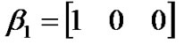
It is assumed that the wireless network can transmit a fixed size data block during one time slot, and each packet is segmented into a number of data blocks. Suppose a station can transmit voice and video traffic. Furthermore, the priority of voice traffic is higher than the video traffic. Voice traffic is modeled by an ON/OFF source as depicted in Figure 4a. Therefore,  and
and  can be calculated as follows [15].
 ,
, 
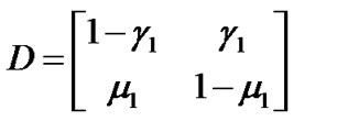
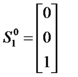
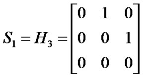
where  is the probability of the packet arrival per time slot. Now assume that the voice packet length is fixed and is three times more than data block size. Therefore,
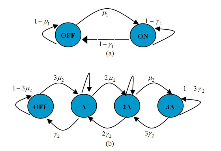
Figure 4. ON/OFF traffic model for Voice and VBR traffic.
The VBR traffic is modeled by three independent ON/OFF sources as showed in Figure 4b. ,
,  and
and  can be easily calculated like voice traffic matrices. Readers to find more details can refer to [15]. If we assume that the maximum video packets size is 8 times more than data block size, and video packets size follow log-normal distribution with a probability mass function (
 ) in terms of the number of data blocks such a following example [3]


The  and
and  will be


Let SI and TXOP durations be 100 and 10 slots, respectively. Then,
 T=10 Using the above information, one can easily find out system performance through the introduced model.
Now, according to the 802.11e and characteristics of the applied traffic streams which are described as follow, the numerical results obtained from the analytical model are compared with simulation results. We analyze the queue length and the access delay distribution as well as the packet loss rate for the high priority and the low priority packets. Similar to above example, one can easily match the proposed model with the introduced traffic and system parameters.
It is assumed that the voice traffic is handled with a higher priority than video traffic. The voice traffic is modeled by an ON/OFF source which generates 160 octet message periodically with a bit rate 64 kb/s during active period. The CBR video traffic has only a ON state and always stays in that. The VBR traffic is modeled by three independent ON/OFF sources with the mean bit rate 200 Kb/s. however, the PhFit program [16] can be used to find out the phase type distribution of service times of real traffic. Table 1 summarizes the different traffic used for the analytical analysis and simulations. It is assumed that the queue buffer size is seven and the channel data rate is 12Mbps.
Simulations are performed using program which is written in C++ medium. There are two queues in each station, and the server processes packets in each of the queues in the FIFO fashion. There are ten stations which are communicating with the access point. All stations enjoy ON/OFF voice traffic as high priority traffic. Five stations generate the CBR video traffic and the others send the VBR video traffic as low priority traffic. Arrivals to the queues are independent of whether the server is in service or on vacation. The TXOPs duration are calculated through Eqn (1), according to the traffic information in each station. Each station can transmit its data during its TXOP period.
Figure 5 shows cumulative distribution function (CDF) of the high priority and the low priority queue length for VBR, CBR video and voice traffic streams. Although the CBR packet arrival rate is much larger than that of the VBR traffic stream, the queue length in the CBR traffic is less than that one in the VBR traffic considerably. As it is obvious from the mentioned figure, the probability that the length of the queue get less than or equal to six is about 98 percent for the CBR traffic while that is about 74 percent for the VBR traffic. It means that most of the time the VBR packets remain in the queue and unable to be transmitted. Therefore, the packet loss goes up and lots of packets drop. Simulation and numerical results show that the packet loss rate is about 28 percent for the VBR traffic while it is about 0.6 percent for the CBR video traffic. Consequently, although there is enough bandwidth to support QoS guarantee in the VBR video traffic but the scheduler is unable to use it.
The CDF of the queue length at the end of the TXOP for all traffic, plotted in Figure 6, confirms created challenges through the VBR traffic. Therefore, the modification of the scheduling algorithm and introduction of a dynamic scheduler to adapt with the bursty arrivals are unavoidable. Dynamic conditions in the scheduler can be obtained through adjusting the TXOP and the SI durations based on the packet queue length statistics. Scheduler can get the information from the stations and find the optimal TXOP and SI through the employing the model to maintain an empty queue at the end of TXOP duration.
Figure 7 shows CDF of the access delay and packet blocking in the high priority and the low priority traffic through analysis and simulations. It is observed that all packets in the CBR video traffic experience access delay less than about 35 ms, while only 23 percent of the VBR video packets experience such a cumulative access delay. Although there is enough bandwidth to serving the VBR traffic, the scheduler does not have essential flexibility to support of bursty arrival rate. Consequently, the queue will be full and 28 percent of arrived packets are blocked and dropped.
Finally, from Figures 5-7, it can be readily seen that the validation of analytical model is confirmed by the numerical results obtained from analytical model and the simulation results under the same conditions.
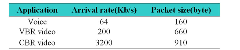
Table 1. Description of different traffic streams.
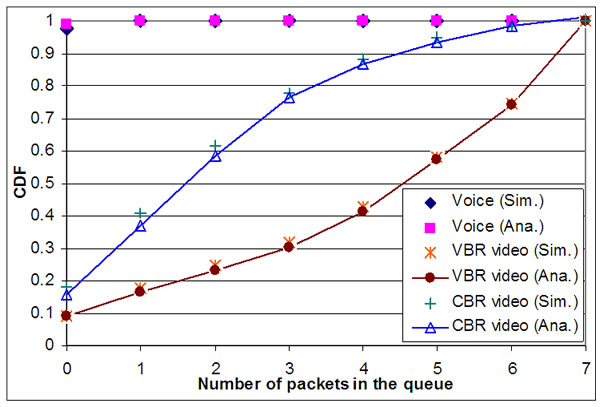
Figure 5. CDF of packet queue length for different traffic streams (Simulation (Sim.) & Analytical (Ana.)).
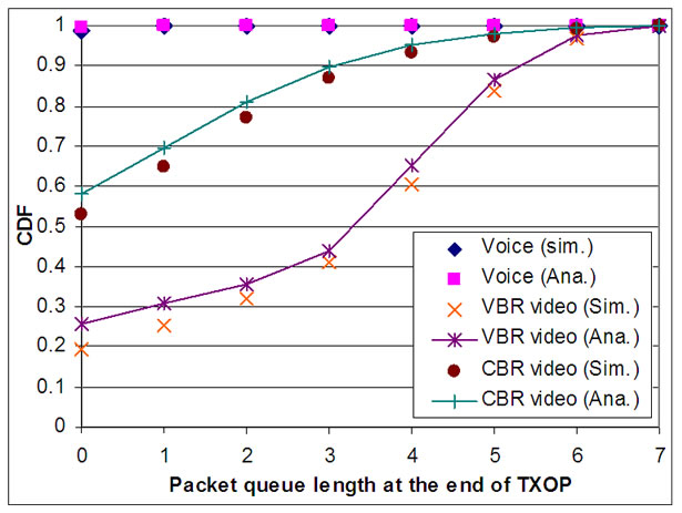
Figure 6. CDF of packet queue length for different traffic streams at the end of TXOP (Simulation (Sim.) & Analytical (Ana.)).
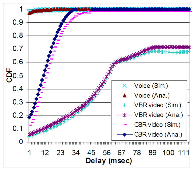
Figure 7. CDF of access delay for different traffic streams (Simulation (Sim.) & Analytical (Ana.)).
6. Conclusions
The scheduling algorithm which is introduced by HCCA /IEEE802.11e to support QoS in multimedia applications enjoys separated queues with specified priority levels and transmission opportunity according to the traffic streams characteristics. The transmission opportunity is found out based on the mean values. Therefore, some multimedia traffic streams such as VBR traffic address some challenges in this medium. Consequently, adapting algorithms to new conditions in order to provide desired QoS is on the focus of researchers. To investigate and improve the scheduler, analytical model is very useful. This paper introduced a priority queuing model for the HCCA. Using of the MAP/PH/1 queue makes the model more comprehensive and provides it to support different practical traffic streams. The important performance measures in the high priority and the low priority queues are calculated which enable us to investigate the effect of the SI and the TXOP durations on QoS guarantees and find out the optimal TXOP values according to the queue length and the access delay statistics to provide QoS. It is shown by the numerical and the simulation results that the analytical model is quite accurate, and thus useful in the practical system design and performance evaluation.
7. Acknowledgments
This work was supported in part by the National Science Foundation of China (NSFC) under the Grant No. 90604035, the 111 Project under the grant No.111-2-14, the National 863 High-Tech R&D Program under the grant No.2007AA01Z228.
8. References
[1] IEEE 802.11e/D13.0, Part 11, Wireless LAN medium access control (MAC) and physical layer (PHY) specifications: Medium access control (MAC) enhance-ments for quality of service (QoS), draft supplement to IEEE 802.11 Std, January 2005.
[2] M. F. Neuts, “Matrix geometric solutions in stochastic models-an algorithmic approach,” John Hopkins University Press Baltimore, MD, 1981.
[3] J. A. Zhao, B. Li, X. Cao, and I. Ahmad, “Matrix-analytic solution for DMAP/PH/1 priority queue,” Queuing Systems Journal, Springer Netherlands, Vol. 53, No. 3, pp. 127-145. July 2006.
[4] S. Mangold, S. Choi, G. R. Hiertz, O. Klein, and B. Walke, “Analysis of IEEE 802.11e for QoS support in wireless LANs,” IEEE Wireless Communications, pp. 40-50, December 2003.
[5] P. Ansel, Q. Ni, and T. Turletti, “FHCF: A Simple and an efficient scheduling scheme for IEEE 802.11e wireless LAN,” Mobile Networks and Applications, No. 11, pp.
391-403, April 2006.
[6] A. Grilo, M. Macedo and M. Nunes, “A Scheduling Algorithm for QoS Support in IEEE802.11e Networks,” IEEE Wireless Communications, pp. 36-43, June 2003.
[7] A. lera, A. Molinaro, G. Ruggeri, and D. Tripodi, “Improving QoS and throughput in single and multihop WLANs through dynamic traffic prioritization,” IEEE Network, pp. 35-44, June 2005.
[8] N. Vaidya, A. Dugar, S. Gupta, and P. Bahl, “Distributed fair scheduling in a wireless LAN,” IEEE Transactions on Mobile Computing, Vol. 4, No. 6, pp. 616-629, Nov-ember 2005.
[9] H. Zhai, X. Chen and Y. Fang, “How well can the IEEE 802.11 wireless LAN support quality of service?” IEEE Transactions on Wireless Communications, Vol. 4, No. 6, pp. 3084-3093, November 2005.
[10] Z. Kong, D. Tsang and B. Bensaou, “Performance analysis of IEEE802.11e contention-based channel access,” IEEE Journal on Selected Areas in Communi-cations, Vol. 22, No. 10, pp. 2095-2106, December 2004.
[11] Y. Xiao, “Performance analysis of priority schemes for IEEE 802.11 and IEEE 802.11e wireless LANs,” IEEE Transactions on Wireless Communications, Vol. 4, No. 4, pp. 1506-1515, July 2005.
[12] H. Zhu and I. Chlamtac, “Performance analysis for IEEE 802. 11e EDCF service differentiation,” IEEE Transactions on Wireless Communications, Vol. 4, No.4, pp. 1779-1788, July 2005.
[13] M. M. Rashid and E. Hossain, “Queuing analysis of 802.11e HCCA with variable bit rate traffic,” IEEE International Conference on Communications, Vol. 10, pp. 4792 -4798, 2006.
[14] A. S. Alfa, “Matrix geometric solution of discrete time MAP/PH/1 priority queue,” Naval Research Logistics, Vol. 45, pp. 23-50, July 1997.
[15] C. Blondia and O. Casals, “Performance analysis of statistical multiplication of VBR sources,” Conference of the IEEE Computer and Communications Societies, pp. 828-838, 1992.
[16] Horvath and M. Telek, “Phfit: A general phase type fitting tool,” in proceedings of 12th performance TOOLS, Lecture Notes in Computer Science, Vol. 2324, London, UK, April 2002.
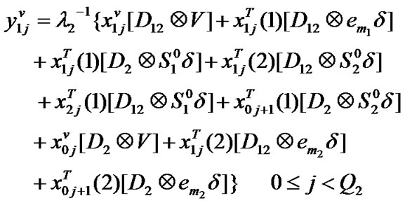
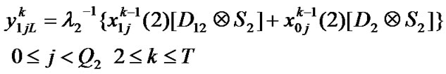
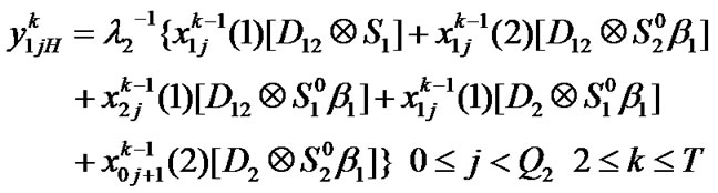
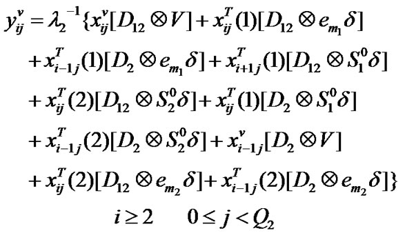
Appendix A
Block matrices of transition matrix P (Section 3.4)


Appendix B
State probability vectors in the high priority access delay (Section 4.3)
Block matrices of transition matrix 
Appendix C
Access delay Distribution for the low priority packets (Section 4.3)
The arriving low priority packet will reach the head of its queue and will be ready to transmit if all the low priority packets ahead of it are served. Since the low priority packet is unable to be transmitted while there are high priority packets in the system, the arriving low priority packet has to wait for completion of the transmission of all high priority and low priority packets which are in the system and those high priority packets which will enter during the period of the time that the arriving packet moves towards head of queue. Therefore, the number of packet ahead of arriving low priority packet at its arrival time is all high priority and low priority packets in the system (including any high priority packet which might have arrived jointly with it). Suppose  defines initial probability vector in the low priority access delay.
 where
where 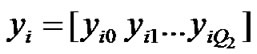
where  represents probability of an arriving low priority packet finding i high priority and j low priority packet in the system with the server on vacation and
  (
( )
) is the probability of an arriving low priority packet finding i high priority and j low priority packet in the system with the server in the low priority (high priority) processing at the kth slot of TXOP. All the probability vectors can be calculated in a similar manner which has discussed in the Section 4.3.


Transition matrix for the low priority packet access delay:

Suppose . Then,
To reduction of computation, the set of following equation can be used.

Finally, let  be the probability that the waiting time of low priority packet is less than or equal to T. Then,
 .
.