Energy and Power En gi neering, 2011, 3, 174-180
doi:10.4236/epe.2011.32022 Published Online May 2011 (http://www.SciRP.org/journal/epe)
Copyright © 2011 SciRes. EPE
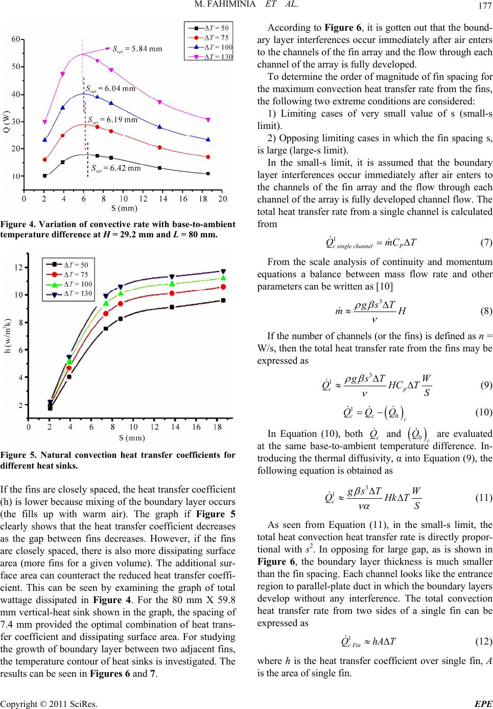
Investigation of Natural Convection Heat Transfer
Coefficient on Extended Vertical Base Plates
Mahdi Fahiminia1, Mohammad Mahdi Naserian2, Hamid Reza Goshayeshi1, Davood Majidian3
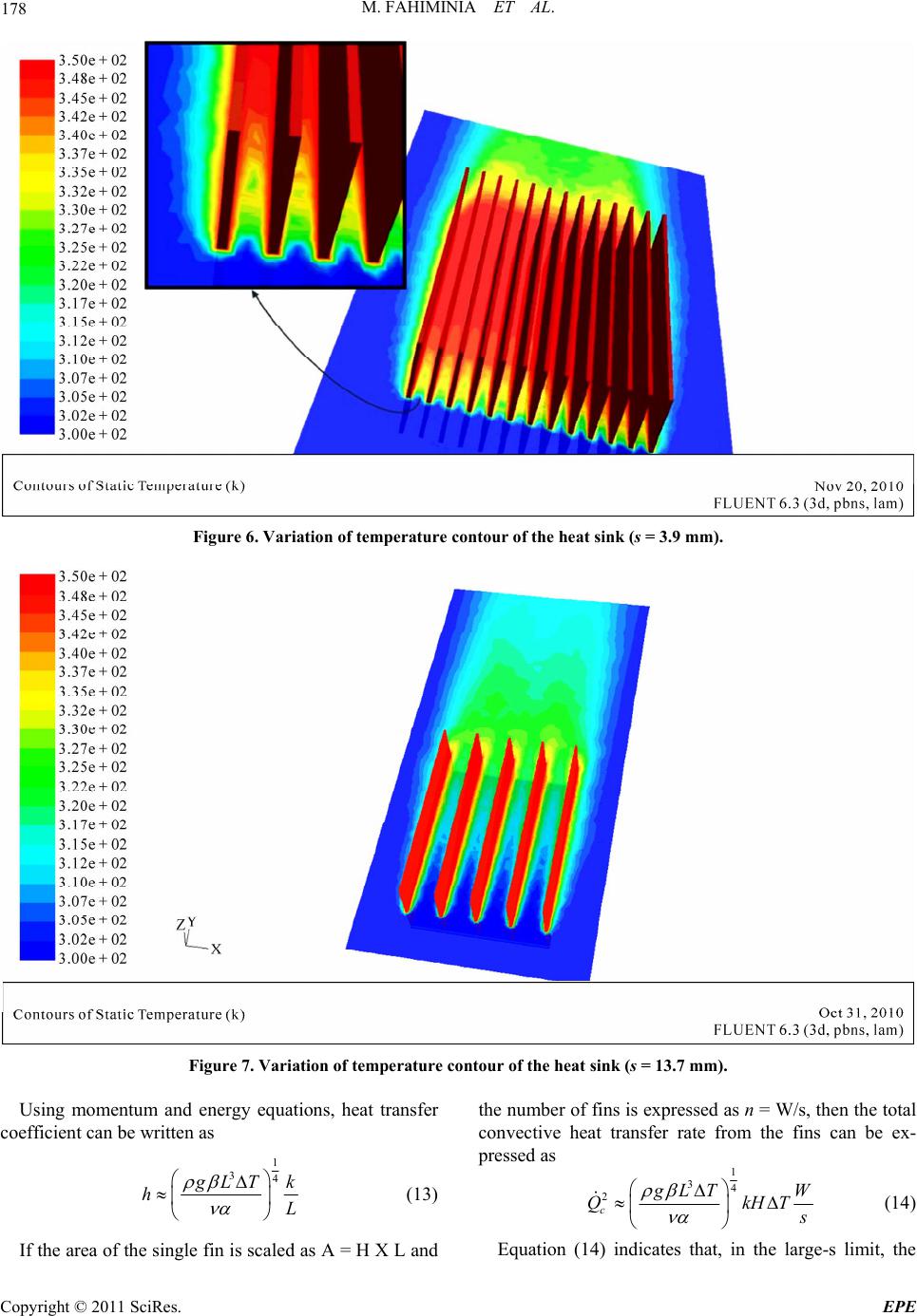
1Department of Mechanical Engineering, Mashhad Branch, Islamic Azad University, Mashhad, Iran
2Young Researchers Club, Mashhad Branch, Islamic Azad University, Mashhad, Iran
3Department of Systems Engineering, Virginia Polytechnic Institute and State University, USA
E-mail: MFahiminia@Gmx.com, Mmahnas@yahoo.com, Goshayshi@yahoo.com, DMajidian@yahoo.com
Received December 21, 2010; revised April 8, 2011; accepted April 15, 2011
Abstract
In this research, computational analysis of the laminar natural convection on vertical surfaces has been in-
vestigated. Natural convection is observed when density gradients are present in a fluid acted upon by a
gravitational field. Our example of this phenomenon is the heated vertical plate exposed to air, which, far
from the plate, is motionless. The CFD simulations are carried out using fluent software. Governing equa-
tions are solved using a finite volume approach. Coupling between the velocity and pressure is made with
SIMPLE algorithm. The resultant system of discretized linear algebraic equations is solved with an alternat-
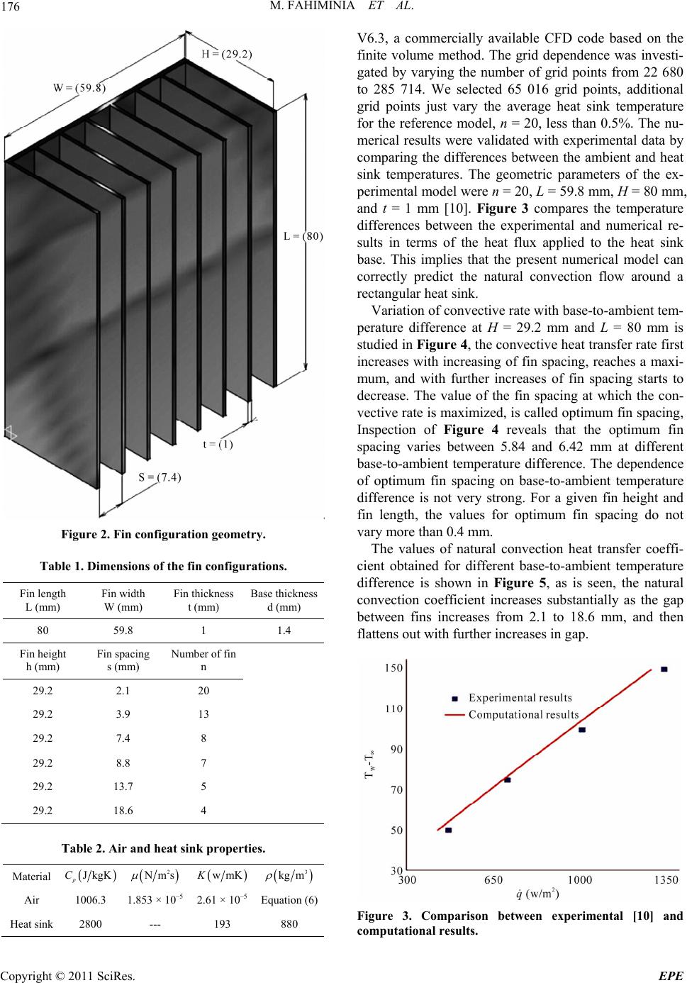
ing direction implicit scheme. Then a configuration of rectangular fins is put in different ways on the surface
and natural convection heat transfer coefficient on these no slope surfaces is studied and finally optimization
is done.
Keywords: Natural Convection, Vertical Surfaces, Simple Algorithm, Rectangular Fins
1. Introduction
In this document Natural convection is observed as a
result of fluid movement which is caused by density gra-
dient. A radiator which is used for warming the house is
an example of practical equipment for natural convection.
The movement of fluid, whether gas or liquid, in natural
convection is caused by buoyancy force due to density
reduction beside to surfaces in heating process. When an
external force such as gravity, has no effect on the fluid
there would be no buoyancy force, and mechanism
would be conduction. But gravity is not the only force
causing natural convection. When a fluid is confined in
the rotating machine, centrifugal force is exerted on it
and if one or more than one surfaces, with more or less
temperature than that of the fluid are in touch with the
fluid, natural convection flows will be experienced. The
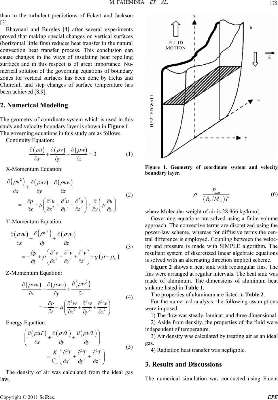
fluid which is adjacent to the vertical surface with con-
stant temperature, the fluid temperature is less than the
surface temperature, forms a velocity boundary layer.
The velocity profile in this boundary layer is completely
different with the velocity profile in forced convection.
The velocity is zero on the wall due to lack of sliding.
Then the velocity goes up and reaches its maximum and
finally gets zero on the external border of velocity
boundary layer. Since the factor that causes the natural
convection, is temperature gradient, the heating bound-
ary layer appears too. The temperature profile has also
the same value as the temperature of wall due to the lack
of particles sliding on the wall, and temperature of parti-
cles goes down as approaching to external border of
temperature boundary layer and it would reach the tem-
perature of far fluid. The initial enlargement of boundary
layer is laminar, but in the distance from the uplifting
edge, depending on fluid properties and the temperature
difference of the wall and the environment, eddies will
be formed and movement to turbulent zone will be
started.
However, relatively little information is available on
the effect of complex geometries on natural convection.
Numerous experimental [1-4] and numerical [5] studies
of rectangular fin heat sinks have been carried out [1].
Since the pioneering experimental work of Ray in 1920,
natural or free convection has developed into one of the
most studied topics in heat transfer. Jofre and Barron
obtained data for heat transfer to air from vertical ex-
tended surface [2]. At RaL = 109 they quoted an im-
provement in the average Nusselt number of about 200%
M. FAHIMINIA ET AL.
175
than to the turbulent predictions of Eckert and Jackson
[3].
Bhavnani and Burgles [4] after several experiments
proved that making special changes on vertical surfaces
(horizontal little fins) reduces heat transfer in the natural
convection heat transfer process. This conclusion can
cause changes in the ways of insulating heat repelling
surfaces and in this respect is of great importance. Nu-
merical solution of the governing equations of boundary
zones for vertical surfaces has been done by Helus and
Churchill and step changes of surface temperature has
been achieved [8,9].
2. Numerical Modeling
The geometry of coordinate system which is used in this
study and velocity boundary layer is shown in Figure 1.
The governing equations in this study are as follows.
Continuity Equation:
  
0
uvw
xyz




(1)
X-Momentum Equation:


2
222
222
uuv uw
xyz
puuu u
x
yy
xyz








 


 


(2)
Y-Momentum Equation:




2
222
222
v
vu vw
xyz
pvvv
g
yxyz







 



(3)
Z-Momentum Equation:


2
222
222
w
wu wv
xyz
p www
z
x
yz





 

(4)
Energy Equation:

222
222
p
uT vTwT
xyy
K
TTT
C
x
yz











(5)
The density of air was calculated from the ideal gas
law,
Figure 1. Geometry of coordinate system and velocity
boundary layer.

atm
cw
P
RM T
(6)
where Molecular weight of air is 28.966 kg/kmol.
Governing equations are solved using a finite volume
approach. The convective terms are discretized using the
power-law scheme, whereas for diffusive terms the cen-
tral difference is employed. Coupling between the veloc-
ity and pressure is made with SIMPLE algorithm. The
resultant system of discretized linear algebraic equations
is solved with an alternating direction implicit scheme.
Figure 2 shows a heat sink with rectangular fins. The
fins were arranged at regular intervals. The heat sink was
made of aluminum. The dimensions of aluminum heat
sink are listed in Table 1.
The properties of aluminum are listed in Table 2.
For the numerical analysis, the following assumptions
were imposed.
1) The flow was steady, laminar, and three-dimensional.
2) Aside from density, the properties of the fluid were
independent of temperature.
3) Air density was calculated by treating air as an ideal
gas.
4) Radiation heat transfer was negligible.
3. Results and Discussions
The numerical simulation was conducted using Fluent
Copyright © 2011 SciRes. EPE
176 M. FAHIMINIA ET AL.
Figure 2. Fin configuration geometry.
Table 1. Dimensions of the fin configurations.
Fin length
L (mm)
Fin width
W (mm)
Fin thickness
t (mm)
Base thickness
d (mm)
80 59.8 1 1.4
Fin height
h (mm)
Fin spacing
s (mm)
Number of fin
n
29.2 2.1 20
29.2 3.9 13
29.2 7.4 8
29.2 8.8 7
29.2 13.7 5
29.2 18.6 4
Table 2. Air and heat sink properties.
Material

JkgK
p
C

2
Nms

wmK
V6.3, a commercially available CFD code based on the
finite volume method. The grid dependence was investi-
gated by varying the number of grid points from 22 680
to 285 714. We selected 65 016 grid points, additional
grid points just vary the average heat sink temperature
for the reference model, n = 20, less than 0.5%. The nu-
merical results were validated with experimental data by
comparing the differences between the ambient and heat
sink temperatures. The geometric parameters of the ex-
perimental model were n = 20, L = 59.8 mm, H = 80 mm,
and t = 1 mm [10]. Figure 3 compares the temperature
differences between the experimental and numerical re-
sults in terms of the heat flux applied to the heat sink
base. This implies that the present numerical model can
correctly predict the natural convection flow around a
rectangular heat sink.
Variation of convective rate with base-to-ambient tem-
perature difference at H = 29.2 mm and L = 80 mm is
studied in Figure 4, the convective heat transfer rate first
increases with increasing of fin spacing, reaches a maxi-
mum, and with further increases of fin spacing starts to
decrease. The value of the fin spacing at which the con-
vective rate is maximized, is called optimum fin spacing,
Inspection of Figure 4 reveals that the optimum fin
spacing varies between 5.84 and 6.42 mm at different
base-to-ambient temperature difference. The dependence
of optimum fin spacing on base-to-ambient temperature
difference is not very strong. For a given fin height and
fin length, the values for optimum fin spacing do not
vary more than 0.4 mm.
The values of natural convection heat transfer coeffi-
cient obtained for different base-to-ambient temperature
difference is shown in Figure 5, as is seen, the natural
convection coefficient increases substantially as the gap
between fins increases from 2.1 to 18.6 mm, and then
flattens out with further increases in gap.
K
3
kg m
Air 1006.3 1.853 × 10⁻⁵ 2.61 × 10⁻⁵ Equation (6)
Heat sink 2800 --- 193 880 Figure 3. Comparison between experimental [10] and
computational results.
Copyright © 2011 SciRes. EPE
M. FAHIMINIA ET AL.
177
Figure 4. Variation of convective rate with base-to-ambient
temperature difference at H = 29.2 mm and L = 80 mm.
Figure 5. Natural convection heat transfer coefficients for
different heat sinks.
If the fins are closely spaced, the heat transfer coefficient
(h) is lower because mixing of the boundary layer occurs
(the fills up with warm air). The graph if Figure 5
clearly shows that the heat transfer coefficient decreases
as the gap between fins decreases. However, if the fins
are closely spaced, there is also more dissipating surface
area (more fins for a given volume). The additional sur-
face area can counteract the reduced heat transfer coeffi-
cient. This can be seen by examining the graph of total
wattage dissipated in Figure 4. For the 80 mm Χ 59.8
mm vertical-heat sink shown in the graph, the spacing of
7.4 mm provided the optimal combination of heat trans-
fer coefficient and dissipating surface area. For studying
the growth of boundary layer between two adjacent fins,
the temperature contour of heat sinks is investigated. The
results can be seen in Figures 6 and 7.
According to Figure 6, it is gotten out that the bound-
ary layer interferences occur immediately after air enters
to the channels of the fin array and the flow through each
channel of the array is fully developed.
To determine the order of magnitude of fin spacing for
the maximum convection heat transfer rate from the fins,
the following two extreme conditions are considered:
1) Limiting cases of very small value of s (small-s
limit).
2) Opposing limiting cases in which the fin spacing s,
is large (large-s limit).
In the small-s limit, it is assumed that the boundary
layer interferences occur immediately after air enters to
the channels of the fin array and the flow through each
channel of the array is fully developed channel flow. The
total heat transfer rate from a single channel is calculated
from
1
c single channelP
QmC
T (7)
From the scale analysis of continuity and momentum
equations a balance between mass flow rate and other
parameters can be written as [10]
3
g
sT
m

H
(8)
If the number of channels (or the fins) is defined as n =
W/s, then the total heat transfer rate from the fins may be
expressed as
3
1
cp
g
sT W
QHC
S

T
(9)

1
0cc c
QQ Q
 
(10)
In Equation (10), both c and
c are evaluated
at the same base-to-ambient temperature difference. In-
troducing the thermal diffusivity, α into Equation (9), the
following equation is obtained as
Q
0
Q
3
1
c
g
sT W
QHk
S


T
T
(11)
As seen from Equation (11), in the small-s limit, the
total heat convection heat transfer rate is directly propor-
tional with s2. In opposing for large gap, as is shown in
Figure 6, the boundary layer thickness is much smaller
than the fin spacing. Each channel looks like the entrance
region to parallel-plate duct in which the boundary layers
develop without any interference. The total convection
heat transfer rate from two sides of a single fin can be
expressed as
1
cFin
QhA
(12)
where h is the heat transfer coefficient over single fin, A
is the area of single fin.
Copyright © 2011 SciRes. EPE
M. FAHIMINIA ET AL.
Copyright © 2011 SciRes. EPE
178
Figure 6. Variation of temperature contour of the heat sink (s = 3.9 mm).
Figure 7. Variation of temperature contour of the heat sink (s = 13.7 mm).
Using momentum and energy equations, heat transfer
coefficient can be written as
1
34
g
LT k
hL




(13)
If the area of the single fin is scaled as A = H Χ L and
the number of fins is expressed as n = W/s, then the total
convective heat transfer rate from the fins can be ex-
pressed as
1
34
2
c
g
LT W
QkHT
s





(14)
Equation (14) indicates that, in the large-s limit, the
M. FAHIMINIA ET AL.
179
convective heat transfer rate from the fins is inversely
proportional with s. In Figure 7, this trend is indicated
by large-s asymptote. The relations obtained for two ex-
treme conditions are two asymptotes of convective heat
transfer, or versus fin spacing. As a result of
the analysis made for the case of small-s limit, it is esti-
mated that the total convective heat transfer rate is pro-
portional with s2. On the other hand, in the case of
large-s limit, the total heat transfer rate is inversely pro-
portional with fin spacing.
1
c
Q
2
c
Q
2
0
cc c
QQ Q
 
(15)
Solving Equation (12) for fin spacing, the order of
magnitude of optimum fin spacing, sopt for maximum
heat transfer rate can be obtained as,
1
c
QQ

2
c
(16)
For dimensionless presentation of the order of magni-
tude of optimum fin spacing, the Rayleigh number is
employed according to its definition.
1
4
opt
L
SRa
L
(17)
As in Figure 4, the investigations show that in the
same fin length and height and constant base-to-ambient
temperature difference, the optimum fin spacing is the
space which is not too large, like Figure 6, nor too small,
like Figure 7, and the value of it, is between these two
values. Figure 8 show the temperature contour of heat
sink with optimum fin spacing.
3
L
g
LT
Ra




(18)
4. Conclusions
From these figures it can also be seen that, at a given fin
height and temperature difference, the convection rates
increases with increasing fin spacing and reaches a
maximum. With further increases of fin spacing, rate
starts to decrease. The occurrence of this maximum has
significant practical applications for optimum perform-
ance of fin-arrays. It would be appropriate to manufac-
ture the fin array with aforementioned fin height and
spacing. The values of coefficient obtained for an ambi-
ent air temperature of 27˚C and plate surface tempera-
tures of 77, 102, 127 and 157˚C appear in Figure 5. As
may be seen, the natural convection coefficient increases
substantially as the gap between fins increases from 2.1
to 18.6 mm, and then flattens out with further increases
in gap. It may be noted that the values shown for a gap of
18.6 mm are within a few per cent of those obtained us-
ing a correlation for an individual vertical plate.
These figures show that, the convective heat transfer
rate from fin arrays depends on fin height, fin length, fin
spacing and base-to-ambient temperature difference. The
convective heat transfer rates from the fin arrays in-
creases with fin height, fin length and base-to-ambient
temperature difference. The heat transfer rate increases
monotonously with temperature difference between fin
Figure 8. Variation of temperature contour of the heat sink.
Copyright © 2011 SciRes. EPE
M. FAHIMINIA ET AL.
Copyright © 2011 SciRes. EPE
180
base and surroundings, Tw-Ta. If the distance between
the fins is selected properly, there will be no interference
between boundary layers of two adjacent fins and the
surfaces. For stating the magnitude of fin spacing for
having the best convection rates of fins, we choose the-
distance between the fins big enough so that the thick-
ness of boundary layer is smaller than the distance be-
tween the fins and increases without any interfering.
5. References
[1] O. G. Martynenko and P. Khramtsov, “Free-Convection
Heat Transfer,” Springer, New York, 2005.
[2] R. J. Jofre and R. F. Baron, “Free Convection to a Roug-
hplate,” American Society of Mechanical Engineers Pa-
per, Vol. 33, No. 67, 1986, pp. 965-981.
[3] E. R. G. Eckert and T. W. Jackson, “Analysis of Turbu-
lent Free Convection Boundary Layer on Flat Plate,”
NCA Report 1015, Vol. 1, No. 2, 1951, pp. 257-261.
[4] A. E. Bergles and G. H. Junkhan, “Energy Conservation
via Management Quarterly,” Progress Report, No. COO-
4649-59, 31 March 1979, pp. 346-348.
[5] S. H. Bhavnani and A. E. Bergles, “Effect of Surface
Geometry and Orientation on Laminar Natural Convec-
tion from a Vertical Flat Plate with Transverse Rough-
ness Elements,” International Journal of Heat Mass
Transfer, Vol. 33, No. 5, 1990, pp. 965-981.
doi:10.1016/0017-9310(90)90078-9
[6] P. E. Rubbert, “The Emergence of Advanced Computa-
tional Methods in the Aerodynamic Design of Commer-
cial Transport Aircraft,” Proceedings of International
Symposium on Computational Fluid Dynamics, Vol. 1,
No. 4, 1984, pp. 42-48.
[7] S. W. Churchill and R. Usagi, “A General Expression for
the Correlation of Rates of Transfer and other Phenom-
ena,” AIChe Journal, Vol. 18, No. 6, 1972, pp. 1121-
1128. doi:10.1002/aic.690180606
[8] H. P. Kavehpour, M. Faghri and Y. Asako, “Effects of
Compressibility and Rarefaction on Gaseous Flows in
Microchannels,” An International Journal of Computa-
tion and Methodology, Vol. 32, No. 7, 1997, pp. 41-47.
doi: 10.1080/10407789708913912
[9] D. D. Gray and A. Giorgini, “The Validity of the Boussi-
nesq Approximation for Liquids and Gases,” Interna-
tional Journal of Heat and Mass Transfer, Vol. 19, No. 5,
pp. 545-551, 1976. doi:10.1016/0017-9310(76)90168-X
[10] B. Yazicioğlu and H. Yüncü, “Optimum Fin Spacing of
Rectangular Fins on a Vertical Base in Free Convection
Heat Transfer,” Journal of Heat Mass Transfer, Vol. 44,
No. 1, pp. 11-21. doi: 10.1007/s00231-006-0207-6
Nomenclature (List of Symbols)
Symbol Quantity Unit
A area m2
h convection heat transfer coefficient w/m2k
T temperature k
Cp specific heat at constant pressure kJ/kgk
g gravitational acceleration m/s2
H fin height m
k thermal conductivity w/mk
L fin length m
m
mass flow rate kg/s
β volumetric thermal expansion coefficient 1/k
n number of fins -
s fin spacing m
t fin thickness m
W base plate width m
1
c
Q
convection rate from fins in small-s limit w
2
c
Q
convection rate from fins in large-s limit w
c
Q
convection rate w
Ra Rayleigh number -
Tw base plate temperature k
Ta ambient temperature k
ν kinematic viscosity m2/s
α thermal diffusivity m2/s