Modern Economy, 2011, 2, 114-123
doi:10.4236/me.2011.22016 Published Online May 2011 (http://www.SciRP.org/journa l/ me )
The Interaction of Monetary and Fiscal Policy: The
Brazilian Case
Tito Belchior Silva Moreira1, Fernando Antônio Ribeiro Soares2, Adolfo Sachsida3,
Paulo Roberto Amorim Loureiro4
1Department of Economics, Catholic University of Brasília, Brasília, Brazil
2Brazilian Ministry of Defense, Bra sília, Brazil
3Instituto de Pesquisa e Economia Aplicada, Brasília, Brazil
4Universidade de Br as ília, Brasília, Brazil
Received December 6, 2011; revised March 18, 2011; accepted M ar ch 20, 2011
Abstract
We tested, empiricall y , wheth er th e Brazilian fiscal po licy for the p erio d between 199 5: I to 2008: III was ac-
tive or passive. To analyze fi scal policy transmissio n mechanis ms, we estimated funct ions by which t he pub-
lic debt/GDP ratio affects investment, primary surplus, output gap and the demand for money. The ratio of
public debt to GDP was found to be statistically significant, positively affecting the demand for money and
the primary surplus, whereas it was found to negatively affect the level of investment and the output gap. We
conclude that the Brazilian reg ime was non-Ricardian in the context of fiscal dominance.
Keywords: Active and Passive Polici es, Non-Ricardian R egime, Public Debt and Fiscal Do mi nance Regime
1. Introduction
Since 1999, Brazil has been under an inflation targeting
regime in an environment of fiscal imbalance, illustrated
by the successive nominal deficits generated in recent
decades.
Despite the successive primary surpluses generated in
recent years and a relatively stable ratio of public debt to
GDP, the trajectory and profile of the Brazilian public
debt continue to constitute a cause for concern, especially
if we consider the rise in the ratio of debt to GDP after
the recent bank crisis/financial crisis (subprime crisis)
that has gripped the world.
The sharp reduction in the level of economic activities
since the last quarter of 2008 due to subprime crisis and
the strong retraction in the Brazilian output growth rates
in 2009 contr i buted to reduce the publ ic revenues, whe re a s
the level of government expenditure increased.
The high interest rates imposed by the Brazilian Cen-
tral Bank (BCB) in order to reach the inflation targets con-
tribute to making the cost of servicing the debt higher
than the primary surplus. Despite the recent reduction in
the nominal interest rate in 2009, Brazil still has one of
the highest real interest rates in the world.
Continuous growth of the nominal deficit and, cones-
quently, of the public debt, makes the fiscal imbalance
particularly worrisome, due to the high public debt stock
and the elevated short-term liabilities in a scenario of
strong retr action of the wor ld economy and, the refore, of
the national economy.
The principal objective of this study was to test, em-
pirically, whether fiscal policies have had, from 1995: I
to 2008: III, an impact on real variables such as the real
demand for money, the ratio of investment to GDP and
the output gap. Hence, we aimed to investigate whether
the Brazilian economy supports the Ricardian equiva-
lence hypothesis. We also test, empirically, whether or
not the monetary and fiscal policies are passive or active
based on Leeper model [1].
To that end, we tested certain non-Ricardian models,
such as those devised by [2-4]. In addition, we aimed to
analyze the transmission mechanisms of fiscal policy by
estimating the relationship between the primary surplus
and public debt, as well as the “fiscal” investmen t -sav -
ings (IS) curve. The use of the term “fiscal” IS was based
on the fact that a fiscal variable was used in the estima-
tion. For the present study, we used the ratio of the pri-
mary surplus to GDP. We also determined whether the
fiscal variable, public debt, was significant and to what
extent it affected the investment rate, the output gap and

T. B. S. MOREIRA ET AL.
115
the demand for money. In other words, we analyzed
whether the fiscal policy was active in the period ana-
lyzed.
The basis of this discussion is the con cept of Ricardian
equivalence, as proposed by [5]. The general principle of
Ricardian equivalence is that the government debt is
equivalent to future taxes and, if consumers are suffi-
ciently prudent, future taxes will be equivalent to current
taxes. Therefore, to finance the government by increase-
ing the debt is equivalent to financing by raising taxes.
The implication of Ricardian equivalence is that fiscal
cuts financed by debt do not alter consumption. Families
save the extra disposable income to pay for the future
fiscal liability caused by the fiscal cuts.
This increase in private savings compensates precisely
for the reduction in public savings. National savings re-
main unaltered. In the present study, we attempted to
determine whether the public debt truly matters.
2. Monetary and Fiscal Policies: A Brief
Discussion
Since the 1970s, Brazil has systematically shown i nternal
or external macroeconomic disequilibrium. This condition
generated substantial inflation. To attenuate this effect,
policymakers resorted to stabilization policies. These
policies frequently result in internal or external debt dis-
equilibrium. One of the possible explanations to the debt
stock disequilibrium is the possible inconsistency be-
tween fiscal and monetary policies.
The debate between monetary and fiscal policies has
been restricted to the discussion between rules versus
discretionary behavior. Nowadays, this discussion has
mainly emphasized the inflation targeting pro posals. The
optimal monetary policy rule as sumes that the fiscal pol-
icy is not relevant to the monetary policy. It is assumed
implicitly that public debt is solvent. In other words, the
fiscal authorities always adjust the taxes in order to
guarantee debt solvency. In fact, in a fiduciary regime,
the debt will always be solvent given that it is possible to
use the seigniorage as source of revenue. With the fiscal
policy neglected, the discussion about coordination be-
tween monetary and fiscal policies is weakened. In this
context, some researchers place emphasis on the discus-
sion related to the coordination between monetary and
fiscal policies to keep economic stability. Sargent and
Wallace [6], for example, discuss this question in their
seminal work related to the unpleasant monetarist arith-
metic.
Reference [6] show that if the monetary policy affects
the extent to which the seigniorage is exploited as a
source of revenue, then the monetary and fiscal policies
should be coordinated. In this sense, the price stabiliza-
tion policy depends on the following question: who acts
first, the fiscal or the monetary authority? Or, who im-
poses discipline on whom? The unpleasant monetarist
arithmetic suggested by the authors appears in a process
of policy coordination in which the fiscal policy domi-
nates monetary policy and the monetary authority con-
fronts itself with restrictions imposed by the demand of
government bonds. This is a possible case of active fiscal
policy and pass ive monet a ry behavior.
Many papers show the equilibrium policy as the result
of a game between fiscal and monetary authorities. Ref-
erence [7], for example, makes the description of a Ri-
cardian regime in which the monetary authority is the
dominant player while the fiscal authority is the follower.
In this sense, the fiscal authority increases the fiscal tax
to satisfy the condition of budget equilibrium. This is an
example of a passive fiscal policy and active monetary
policy.
According to [1], what distinguishes an active policy
from a passive one is the fact that the active policy takes
into account the expected future while the passive one
relies on the behavior of current and past values of eco-
nomic variables. Thus, an active policy is not restricted
by current conditions and may well include a choice of a
decision rule that depends on past, current or future val-
ues of economic variables.
A passive policy or passive authority (fiscal or mone-
tary), on the one hand, is restricted by decisions of con-
sumer optimization and by the actions of the active au-
thority, on the other hand. If the fiscal policy is passive,
for example, the decision rule of the fiscal authority will
necessarily depend on the public debt, current or past.
Reference [8] emphasizes that the discussion related to
fiscal dominance is not new. It appeared in the literature
in the works such as [6,9]. Reference [9] states that the
price of bonds is analogous to the price level, and the
nominal rate of interest is determined by the bond/money
ratio and bears no close relationship to the rate of expan-
sion of the price level. The recent developments were
started with the Fiscal Th eory of the Price Level (FTPL)
of [10]. The studies of [1,11-18] concentrate on the dis-
cussion about coordination and interaction between the
monetary and fiscal policies.
The main point emphasized by the research on the
FTPL is that the intertemporal government budget con-
straint and the fiscal policy are the determining factors
for the price level. This argument runs counter to the tra-
ditional theory of price determination, in which the stock
of money and the monetary authority are the only deter-
minant of the price level. Moreover the fiscal policy, ex-
plicitly or implicitly, passively adjusts the primary sur-
plus to guarantee government solvency for any price
level. Since the fiscal authority is free to choose the pri-

T. B. S. MOREIRA ET AL.
116
mary surplus, independently of the government debt,
then it is the price level th at has to adjust itself to satisfy
the intertemporal government budget constraint in a way
that there is only one price level compatible with the
equilibri um.
The FTPL can be understood, in a simplistic way, as
an application of one of the aspects discussed by [6],
where the fiscal policy imposes restrictions on the extent
of results from the monetary policy.
The main distinction between the classic theory and
FTPL lies in the interpretation of the intertemporal gov-
ernment budget. According to the monetarist tradition,
the government intertemporal equation is a constraint that
is assured for any price level. According to the FTPL, the
government intertemporal equation is an equilibrium
condition determining the equilibrium price lev e l.
The distinction between Ricardian and non-Ricardian
regimes brings important implications to economic poli-
cies. Based on the Ricardian regime, a good monetary
policy is a necessary and sufficient condition to guaran-
tee low inflation. An independent central bank, with a
strong institutional commitment towards price stability,
should compel the fiscal authority to adopt a responsible
and appropriate fiscal policy. For the non-Ricardian re-
gime, a good monetary policy is not a sufficient condi-
tion to ensure low inflation, unless additional measures
are taken into consideration to restrict the freedom of the
fiscal authority.
3. Methodological Aspects
The principal source of the quarterly database regarding
the period between 1995:I and 2008:III was the Instituto
de Pesquisa Econômica Aplicada (IPEA)1. The variables
collected from the IPEA database and adopted in the
present study, as well as their respective abbreviations
(in parentheses), were as follows: money supply (M) -
end of p eriod - in millions of Br azilian Reals (R$); GDP
(Y) - market prices - in millions of R$; nominal interest
rate (R) - over/SELIC - in %; investment (I) or gross
formation of fixed capital, in millions of R$; amplified
consumer price index (P); nominal R$/US$ exchange
rate (E), as official rate, purchase price and mean; real
effective exchange rate (e); primary surplus (PS) in mil-
lions of R$, and the direct tax (
τ
) in millions of R$ is
given by the sum of income and land taxes. As a proxy
for the public debt, we used the federal government bonds
and open market operations (B), the source of which is
the BCB.
We also used a dummy variable to distinguish be-
tween the period of the fixed exchange rate regime (1995:
I to 1998: IV) and the subsequent period of the “flexible”
exchange rate. The real GDP was calculated according to
the implicit GDP deflator. The Hodrick-Prescott filter
was used in order to calculate the output gap (y) defined
as the difference between the real GDP and the potential
GDP (trend). A positive value indicates excess demand.
To calculate the real interest rate (r) the Amplified Con-
sumer Price Index was used. The real interest rate was
calculated in the tradition al mann er, in which
( )
1t R+ =
()( )
1
1 *1π
t tt
rE
+

++

, assuming that
( )
11
ππ
tt t
E
++
=.
The estimated time series models are described in item
4. We used the Johansen cointegration test and the unit
root test, as well as models of simultaneous equations,
such as the generalized method of moments (GMM) with
instrumental variables. The long-term equations resultin g
from the cointegration tests were analyzed, focusing es-
pecially on whether the public debt was significant and
presented the sign expected based on the theoretical
model. Other standard techniques for time series, such as
tests of weak exogeneity, were also used. The economet -
ric techniques used in the present study have been widely
applied and are described in various books on the subject
([19-22 ]).
We used the GMM with instrumental variables to es-
timate a system of equations. When the variables are not
stationary, one can expect specific problems regarding
the conventional inference procedures based on ordinary
least squares regression. Reference [20] stating that it
was necessary to know whether similar problems arose
in the context of two-stage lea st squar es regression when
facing such problems. This has been investigated by [23]
and [24], who concluded that inferences with two-stage
least squares estimators using instrumental variables
were still valid, even in cases of non-stationary or non-
cointegrated series. In this context, the conclusions
drawn by [23,24] are also valid when the GMM is ap-
plied.
4. The Non-Ricardian Models and Their
Empirical Resu lts
In the next four subsections we estimated functions by
which the public debt/GDP ratio affects investment, de-
mand for money, primary surplus and output gap to ana-
lyze fiscal policy transmission mechanisms.
4.1. Effect of the Public Debt on Investment
Reference [2] demonstrated that it is possible to have
sustainable long-term growth in a model of a sector in
which generations overlap. They assume the presence of
a convex technology, without redistribution of income
from the older to the younger generation, with taxation
via income tax and without the pure altruism of [5].
1Institute for Applied Economic Research.

T. B. S. MOREIRA ET AL.
117
Working with the so-called “AK” production function
and assuming the hypothesis that the utility function of
the agent incorporates an absolute bequest motive, ref-
erence [2] derives a clear implication of the model po licy,
i.e., an increase in the government debt adversely affects
the rate of growth of the capital stock, as exemplified in
the following equation:
()( )
11
1
1
1 11
t ttt
t
K KBK
A
KA
δ
δδ
−−
−
−−
= −
+ ++
(1)
where Kt is the capital stock at the beginning of period t;
Bt is the stock of government debt bonds at the beginning
of period t; A represents technology; and the coefficient
δ
indicates the preferences of the agents.
This equation shows that the rate of growth of the cap-
ital stock is endogenous. In this context, the public debt as
a proportion of the capital stock in the previous period
adversely affects the rate of capital accumulation.
Considering that the difference between the capital
stock in t and the capital stock in (t − 1) is the investment
(1
tt t
KK I
−
−=
), and that
11tt
Y AK
−−
=
, Equation (1) can
be rewritten as follows:
( )
1 011
*
tt tt
IYBY ββ
−−
= + (2 )
where
() ()
0
11AA βδ δ =−+
and
()( )
1
11 1A βδ =−++ 

. The equation can then be esti-
mated with log-transformed variables, as follows:
( )
1 011
*
tttt t
IYBY u ββ
−−
=++
(3 )
where the parameter 1 β shows the relationship b etween
the ratios of debt (t) to GDP (t − 1) and of investmen t (t)
to GDP (t − 1); 0 β
is the intercept parameter; and t
u
is the error (stochastic term).
We then determined whether the parameter 1 β
was
statistically significant, that is, whether it was different
from zero, and its respective sign. If 1 β
is negative and
statistically significan t, we can infer that the ratio of debt
to GDP negatively affected the ratio of investment (t) to
GDP (t − 1). In other words, if 1 β
= 0, the hypothesis
of Ricardian equivalence can be established.
We initially determined whether the aforementioned
variables were stationary. In case the variables were not
stationary, we attempted to determine whether they were
cointegrated. The table presented in Appendix shows that
both variables were non-stationary. Therefore, we needed
to employ a cointegration test to determine whether the
regression was validated, i.e., whether or not the regres-
sion was spurio us.
The Johansen cointegration test showed that there was
a cointegration equation with a level of significance of
5%, as shown in the Tables A.2 and A.3 in Appendices .
A dummy variable was used (as an exogenous variable
in the VAR model used in the present study) to distin-
guish between the period of the fixed exchange rate re-
gime (1995: I to 1998: IV) and the subsequent period of
the “flexible” exchange rate.
The resulting long-term equation showed that the pa-
rameter 1
β was statistically significant, as follows:
( )
() ()
11
1.621 0.220
0.073 0.116
tt tt
IYBY
−−
=−−
(4 )
The values in parentheses represent the standard de-
viations of the respective coefficients estimated. Ac-
cording to the long-term equation, we observed that for
each 1% increase in the ratio of debt (t) to GDP (
1t−
)
there was a 0.22% reduction in the ratio of investment (t)
to GDP (
1t−
). The negative correlation (Pearson) be-
tween these two variables was of −27.3%, at a level of
significance of 5%. In addition, based on the chi-square
statistic (1.819), th e null hypothesis of weak endog eneity
was not rejected (p = 0.177), i.e., the ratio of debt (t) to
GDP (
1t−
) was weakly exogenous.
We observed that the public debt did affect the real
variable in the economy, i.e., the ratio of investment to
GDP. Such empirical evidence suggests the need for a
clear public policy prescription: the government should
aim to reduce the ratio of debt to GDP. A reduction in
the ratio of debt to GDP translates to a higher invest-
ment/GDP ratio.
4.2. Effect of the Public Debt on the Demand for
Money
Reference [3] defined the real demand for money as a
function of a negative relationship with the nominal in-
terest rate and a positive relatio nship with output and r eal
wealth2. Real net wealth is defined using the following
equation:
( )
W MPBP β = + (5)
where W is the value of real net wealth of private agents;
β
is the fraction of government bonds that private
agents perceive as net wealth (
01 β ≤≤
); B is the nomi-
nal stock of government debt bonds; Y/P is the real out-
put; R is the nominal interest rate; P is the price level;
and M is the no minal money supply. Therefore, the defi-
nition of real demand for money is given by this equa-
tion:
( )()
1 23
MPLYPLRL MPBP β = +++


(6)
According to [3], after dividing Equation (6) by Y/P
we would have the fol l owing equation:
( )
12 3
mLLRL mb β =++ + (7)
2Reference [4] employed a similar app roach to the real demand for mo-
ney in the context of non-Ricardian equivalen ce.

T. B. S. MOREIRA ET AL.
118
where 10
L
>, 20
L
< and 30
L
>;
m MY
=; and
b BY
=.
Equati on ( 7) can be rewritten as:
() ()()
1323 33
11 1m LLLLRLLb β = −+− +−
(8)
On the bas is of Equation (8) , we can defin e a stochas-
tic equation:
01 2tt tt
m Rb βββ η
=+++
(9 )
where
( )
01 3
1
LL
β =− ,
( )
12 3
1
LL
β =− and
( )
2 33
1LL ββ = −
.
If
2
β
was statistically equal to zero, the hypothesis
of Ricardian equivalence was established. We estimated
Equation (10) with log-transformed variables. The table
in Appendix A.1 shows that m, b and R were not station-
ary. The Johansen cointegration test showed that there
were two cointegration equations at a level of signify-
cance of 5%, as shown in the Tables A.4 and A.5 in
Appendices. We again used the dummy variable as an
ex- ogenous variable in the VAR model. The long-term
equation showed the following:
() ()()
1.924 0.2860.820
0.088 0.087 0.114
t tt
m Rb=−− + (10)
The values in parentheses represent the standard de-
viations of the respective coefficients estimated. Ac-
cording to the long-term equation, we noted that for each
1% increase in the ratio of debt to GDP there was a
0.82% increase in the demand for money. There was a
positive correlation (Pearson) of 94.2% between these
two variables at a level of significance of 1%. On the
basis of the chi-square statistic (15.197), the null hypo-
thesis of weak endogeneity of the ratio of debt to GDP
was rejected (p < 0.001). As expected, there was a nega-
tive correlation between the interest rate and the demand
for money. We observed that for each 1% increase in
nominal interest rate there was a 0.286% reduction in the
demand for money.
4.3. Effect of the Public Debt on the Primary
Surplus
Reference [25] evaluated the sustainability of the fiscal
policy based on the response of the primary surplus (ex-
cept fo r interest rates)/GDP ratio to changes in the public
debt/GDP ratio. We simplified this relatio nship through a
regression with log-transformed varia bles as follows:
() ()
0.004 0.031*
0.0020.003
PSYB Y= +
(11)
The Tables (A.6) and (A.7) in the appendices show
that both variables were I(1), and that they cointegrated
at a level of significance of 5%. The values in parenthe-
ses represent the standard deviations of the respective
coefficients estimated.
According to the long-term equation, we noted that for
each 1% increase in the ratio of debt to GDP there was a
0.031% increase in the ratio of the primary surplus to
GDP. The positive correlation (Pearson) between the two
variables was 74.7%, at a level of significance of 5%.
We also observed that, based on the chi-square statistic
(1.168), the null hypothesis of weak endogeneity was not
rejected (p = 0.279), i.e., the ratio of debt to GDP was
weakly exogenous.
4.4. Effect of the Public Debt on the Primary
Surplus and on the Output Gap
In this section, we estimated the equations of the fiscal IS
and of the relationship between the primary surplus and
public debt. The most appropriate method of estimating
these two equations as a system was using the GMM,
with appro pr iat e instr u ment al var iable s. All v ariables were
log-transformed. The estimation of the equation to mea-
sure the response of the primary surplus/GDP (PS/Y)
ratio to the levels of the government debt/GDP (B/Y) ratio
was defined as follows:
( )( )()
01 2 1
1t t tt
PS YaaPSYaBYu+
+
=+ ++
(12)
where ut is the stochastic term.
The fiscal IS was defined as:
( )
1345 671tt ttt
t
yaayaraPSYa e η
++
=+ ++++
(13)
where yt is the output gap; rt is the real interest rate;
(PS/Y)t is the fiscal variable of interest (primary sur-
plus/GDP); et is the real exchange rate; and 1t
η
+ is the
stochastic term.
The use of the denomination fiscal IS was due to the
fact that we considered a fiscal variable in the IS curve.
We assumed that the stochastic terms of Equations (12)
and (13) were not serially correlated.
On the basis of this model, we identified the direct ef-
fects of the public debt on the primary surplus and the
indirect effects of the public debt on the output gap. If
the ratio of public debt to GDP was statistically signify-
cant in Equation (1 2) and the ratio of the pr imary surplus
to GDP was also statistically sign if icant in Equation (13),
we would have an indication that the fisc al policy was ac -
tive. That meant that the government debt indirectly af-
fected a real variable (output gap) via the primary surplus.
The results presented in Table 1 show that all vari-
ables were statistically significant to a level of 1% and
that each 1% increase in the ratio of debt to GDP trans-
lated to a 0.023% increase in the ratio of the primary
surplu s to GDP.

T. B. S. MOREIRA ET AL.
119
The GMM applied in combination for the two equa-
tions in the form of a system, yielded the results pre-
sented in Tables 1 and 2. The model specification was
tested using the J statistic associated with overide ntifica-
tion restrictions. The value of the J statistic was 0 .28 (p =
0.50), and there was therefore no basis for rejecting the
model specification.
The results presented in Table 2 also showed that all
variables were statistically sign ificant to the level of 5%.
In short run, an increase of 1% in the ratio of the primary
surplus to GDP caused a reduction of 2.963% in the
output gap, so that the final effect of the 1% increase in
the ratio of debt to GDP was a 0.07% reduction in the
current output gap. In the long term, considering the ef-
fect of the coefficient for the lagged output gap, the fin al
effect would be a reduction of 0.31% in the output gap.
This result provided empirical evidence that the fiscal
policy was active.
The remaining coefficients showed the expected signs,
so that each 1% increase in the real interest rate ca used a
0.048% reduction in the output gap and each 1% increase
in the real exchange rate caused a 0.006% increase in the
output gap.
Table 1. GMM estimate using t he Bartlett kernel and a fixed
bandwidth:
( )( )( )
=+ ++
1
01 2
1 t t tt
PS YaaPSYaBYu
+ +
.
Variable Coefficient Standard
deviation t statistics p-value
Intercept 0.004 < 0.001 18.045 < 0.001
PS/Y 0.221 0.026 8.411 < 0.001
B/Y 0.023 < 0.001 27.670 < 0.001
R2 0.612
Note: instruments: y(–3, –4, –5, –6), r(–3, –4, –5, –6), PS/Y(–3, –4, –5, –6),
e(–3, –4, –5, –6), B/Y(–3, –4, –5, –6), c.
Table 2. GMM estimate using the Bartlett kernel and a fix-
ed bandwidth:
( )
345 67tt t
t
=+ +++
1t
yaaya raPSYae
+
( )
++ +
1
12
η
t
tt
a BYu
+
+
.
Variable Coefficient Standard
deviation t statistics p-value
Intercept 0.431 0.029 15.047 <0.001
Y 0.771 0.013 59.371 <0.001
R −0.048 0.009 −5.316 <0.001
PS/Y −2.963 0.250 −11.836 <0.001
E 0.006 0.003 2.091 0.039
R2 0.722
Note: instruments: y(–3, –4, –5, –6), r(–3, –4, –5, –6), PS/Y(–3, –4, –5, –6),
e(–3, –4, –5, –6), B/Y(–3, –4, –5, –6), c.
5. The Leeper’s Model and the Empirical
Results
The model developed by [1] defines the conditions ac-
cording to which the monetary and fiscal policies may be
classified as passives and/or active, where
B
is the gov-
ernment nominal debt, on which a nominal interest rate
t
R
is paid,
τ
is the direct lump-sum tax,
p
is the
price level, 1
πt tt
pp
−
= and
t tt
b Bp=
.
The author describes government policies based on
simple rules where the fiscal policy is:
01t tt
B τγγ
−
= ++Ψ
(14 )
where t
Ψ is the exogenous shock, occurring at the be-
ginning of t and following the AR(1) process:
1
t tt
ρε
Ψ− Ψ
Ψ=Ψ+ (15)
with
1 ρ
Ψ
<
and 10
tt
E ε
Ψ+ =.
We believe that it makes more sense to consider direct
taxes and the nominal government debt relative to GDP.
Equati on ( 14 ) be c omes:
1
01
tt
t
tt
Bu
GDP GDP
τγγ
−
−
=++
(16)
where
t
u
is the stationary AR(1).
The monetary policy also obeys a simple rule for the
interest rate, that is,
π
to tt
R αα = ++Θ
(17)
where t
Θ is an exogenous shock, occurring at the be-
ginning of t and following the AR(1) process:
01
t tt
θ
ρε
−
Θ=Θ + (18)
with 01 ρ < and 10
tt
E
ε
Θ+ =.
Leeper’s approach reduces the equilibrium solution of
his model to a dynamic system in
( )
π,
tt
b and finds the
roots
αβ
and
1
βγ
−
−
. The stability condition requires
one root less than or equal to one in absolute value and
another greater than or equal to one. It follows that the
equilibrium generates four regions of i nt e rest.
1) Region 1: 1 αβ ≥ and 11
βγ
−
−<
. This is the
case of a unique equilibrium. In this region, the
Ricardian equivalency holds. In this context, the
monetary policy is active and the fiscal policy is
passive. This is the ideal region for the policy-
maker to instate a target of inflationary regime con-
trolling the interest rate;
2) Region 2: 1 αβ < and 11
βγ
−
−≥
. This region
also generates a unique equilibrium. The region II
represents the fiscal theory of price level (FTPL) or
the regime of fiscal do minancy. In this case, on e has
a passive moneta ry policy and an acti ve fiscal policy;
3) Region 3: 1 αβ < and 11
βγ
−
−<
. In this re-
gion, the fiscal and monetary authorities act pas-

T. B. S. MOREIRA ET AL.
120
sively, subject to the budget constraint. In this case,
there are an infinite number of equilibrium points,
which means that the equilibrium is undetermined;
and
4) Region 4: 1 αβ ≥ and 11
βγ
−
−≥
. There is no
equilibrium in this region unless the exogenous
shocks,
t
ψ
ε
and
t
θ
ε
, are perfectly correlated. In
this case, the monetary and fiscal policies are active.
The discussion above implies important consequences
for the policy-making decisions. The optimal monetary
policy rules, in the context of inflation targeting regime,
assume, explicit or implicitly, that the economy is oper-
ating in Region 1.
On the other hand, if we assume that the economy is
operating in Region 2, where FTPL dominates, an op-
timal monetary policy rule defined by the control of the
interest rate via Taylor rule does not make sense. In Re-
gion 2, the price level is determined by the fiscal policy,
and the monetary policy is ineffective given that it is
passive. In a context of a non-Ricardian regime, refer-
ence [8] suggests an optimal fiscal rule to control infla-
tion.
In Regions 3 and 4, coordination between the mone-
tary and fiscal authorities is necessary to force the eco-
nomy to migrate to Region 1.
In this section, we estimated two systems of equation to
obtain the parameters
γ
and
α
of the Equation (16) and
(17) via GMM. The first system shows the equation used
by [26] to analyzing the solvency of public debt such as:
( )( )
01 23
1t tt
B YaaTrendaB Yadummyu
−
=+++ +
(19)
and the Equation (16 ) .
The results presented in Table 3 show that all vari-
ables were statistically sign ifican t to a level of 5% except
the intercept and that each 1% increase in the lagged
ratio of the debt to GDP translated to a 0.717% increase
in the ratio of the current debt to GDP. In this case,
eventual insolvency will occur if 10a≠, that is there is
a deterministic trend ([26]).
Table 3. GMM estimate using t he Bartlett kernel and a fixed
bandwidth:
( )( )
1
=++
01 2
t t-
BYaaTrenda BY
*++
4t
aDummy u
.
Variable Coefficient Standard
deviation t statistics p-value
Intercept 0.001 0.021 0.057 0.955
Tend 0.001 < 0.001 2.064 0.042
(B/Y)(-1) 0.717 0.043 16.847 < 0.001
Dummy 0.146 0.031 4.636 < 0.001
R2 0.968 R2 adjusted 0.966
Note: Instruments: B/Y(–3, –4, –5, –6),
τ
/Y (–3, –4, –5, –6), c.
The GMM applied in combination for the two equa-
tions in the form of a system, yielded the results pre-
sented in Tables 3 and 4. The model specification was
tested using the J statistic associated with overide ntifica-
tion restrictions. The value of the J statistic was 0 .20 (p =
0.97), and there was therefore no basis for rejecting the
model specification.
The results presented in Table 4 show that all vari-
ables were statistically significant to a level of 1% and
that each 1% increase in the ratio of the lagged debt to
GDP translated to a 0.005% increase in the ratio of the
direct taxes to GDP. This implies that
0.005 γ =
.
The second system shows two equations: the IS curve
and the Taylor rule. The IS equation is:
12131 415ttttt
yaaya ra eaDummy
η
−− −
=+++ ++
(20)
and the Taylor rul e is defined a s follow:
( )
6 71891
π
tttttt
RaaEay aR η
+−
=+++ +
(21)
where
( )
1
π
tt
E
+
is the expected inflation rate.
The results presented in Table 5 show that all vari-
ables were statistically significant to a level of 1% and
all the coefficients showed the expected signs.
The GMM applied in combination for the two equa-
tions in the form of a system, yielded the results presented
in Tables 5 and 6. The model specification was tested
using the J statistic associated with overidentification
Table 4. GMM estimate using the Bartlett kernel and a
fixed bandw i dt h:
( )( )
*=++
34 -1 t
tt
Ya aBY τη
.
Variable Coefficient Standard
deviation t statistics p-value
Intercept 0.006 < 0.001 27.282 < 0.001
(B/Y)(-1) 0.005 < 0.001 10.035 < 0.001
R2 0.386 R2 adjusted 0.373
Note: Instruments: B/Y(–3, –4, –5, –6),
τ
/Y(–3, –4, –5, –6), c
Table 5. GMM estimate using t he Bartlett kernel and a fixed
bandwidth:
12131415
*
tt t−−−
=+++ ++
tt
yaay arae aDummy η
.
Variable Coefficient Standard
deviation t statistics p-value
Intercept 0.8555 0.096 8.947 < 0.001
1t
y− 0.331 0.077 4.312 < 0.001
1t
r− –0.236 0.031 –7.612 < 0.001
1t
e−
0.111 0.028 3.971 < 0.001
Dummy 0.274 0.036 7.659 < 0.001
R2 0.505 R2 adjusted 0.460
Note: Instruments: R(–2, –3, –4, –5, –6),
π
(–2, –3, –4, –5, –6), B/Y(–2,
–3, –4, –5, –6), c.

T. B. S. MOREIRA ET AL.
121
Table 6. GMM estimate using t he Bartlett kernel and a fixed
bandwidth:
( )
-1
* **=++++
67189
π
ttttt t
RaaE ayaR
+
η
.
Variable Coefficient Standard
deviation t statistics p-value
Intercept –0.315 0.054 –5.835 < 0.001
( )
1
π
tt
E
+
0.149 0.038 3.940 < 0.001
t
y
0.177 0.033 5.398 < 0.001
1t
R− 0.872 0.026 34.070 < 0.001
R2 0.789 R2 adjusted 0.775
Note: Instruments: R(–2, –3, –4, –5, –6),
π
(–2, –3, –4, –5, –6), B/Y(–2,
–3, –4, –5, –6), c
restrictions. The value of the J statistic was 0.25 (p =
0.90), and there was therefore no basis for rejecting the
model specification.
The results presented in Table 6 show that all vari-
ables were statistically significant to a level of 1% and
all the coefficients showed the expected signs. We as-
sume that
( )
11
ππ
tt t
E
++
=. Noticing that an increase of
1% in the expected inflation rate generate an increase of
0.149% in the nominal interest rate. This implies that
0.149 α =
.
The value of
0.98 β =
, the rate of time preference,
was taken from [27]. With
0.005 γ = −
,
0.149 α =
and
0.98 β =
, the Brazilian economy, in the analyzed period,
was in Region 2, where 1 αβ < and 11
βγ
−
−>
.
What can be concluded is that, in the analyzed period,
Brazil was operating in a situation of fiscal dominance.
We estimated the Taylor rule without the output gap, in
according to Equation (17), and we also obtain the same
result, i.e., 1 αβ <.
6. Conclusions
The results show that public debt plays a key role in de-
termining variables such as the real demand for money,
the ratio of investment to GDP and the output gap. In the
period between 1995: I and 2008: III, we observed a pos-
itive correlation b etween the ratio of p ublic debt to GDP
and the demand for money normalized to the GDP. We
also observed that there was a negative correlation be-
tween the ratio of public debt to GDP and the ratio of
investment to GDP, and a negative correlation between
the ratio of public debt to GDP and the output gap. In
this context, we found empirical evidence that the Bra-
zilian economy in the period considered did not corro-
borate the hypothesis of Ricardian equivalence.
In addition, it was observed that the ratio of the pri-
mary surplus to GDP during this same period reacted
positively and directly to an increase in the ratio of pub-
lic debt to GDP, and that the ratio of debt to GDP nega-
tively and indirectly affected the output gap via the pri-
mary surplus. Such results once again provide empirical
evidence that the Brazilian economy did not conform to
the regime of Ricardian equivalence.
On the basis of our findings, we can also infer that
there are strong empirical evidences that the fiscal policy
was active and the monetary policy was passive based on
Leeper model. Reference [28] found similar results.
When there is a Ricardian regime, which implies that
the monetary policy is active and the fiscal policy is pa s-
sive, it is reasonable to only analyze the transmission
mechanisms of the monetary policy. However, in the
case of a non-Ricardian regime, in which the fiscal poli-
cy was active and the monetary policy was passive, we
can and must analyze the transmission mechanisms of
the fiscal policy. Therefore, we can infer that if the pub-
lic debt positively affects the demand for money, it might
also affect the interest rate. Given the money supply, if
there is an increase in the demand for money caused by
an increase in the public debt, a rise or a pressure in the
interest rate is expected. Higher interest rates tr anslate to
reduce levels of investment and, in turn, reduced levels
of output or an output gap. We observed that the public
debt negatively affected the level of investment and the
output gap. These links show how the effects of the fiscal
policy are expanded or transmitted within the economy.
7. References
[1] E. M. Leeper, “Equilibria under ‘Active’ and ‘Passive’
Monetary and Fiscal Policies,” Journal of Monetary Eco-
nomics, Vol. 27, No. 1, February 1991, pp. 129-147.
[2] J. T. Araújo and M. A. C. Martins, “Economic Growth
with Finite Lifetimes,” Economics Letters, Vol. 62, No. 3,
March 1999, pp. 377-381.
doi:10.1016/S0165-1765(99)00013-0
[3] R. D. Kneebone, “On Macro-Economic Instability under
a Monetarist Policy Rule in a Federal Economy,” The Ca-
nadian Journal of Economics, Vol. 22, 1989, pp. 673-
685.
[4] W. M. Scarth, “Macroeconomics: An Introduction to Ad-
vanced Methods,” Harcourt Brace & Company, Toronto
and Orlando, 1996.
[5] R. J. Barro, “Are Government Bonds Net Wealth?” The
Journal of Political Economy, Vol. 82, No. 6, Novem-
ber-December1974, pp. 1095-1117. doi:10.1086/260266
[6] T. J. Sargent and N. Wallace, “Some Unpleasant Mone-
tarist Arithmetic,” Quarterly Review, Federal Reserve
Bank of Minneapolis 5, 1981, pp. 1-17.
[7] T. J. Sargent, “Reaganomics and Credibility, Rational
Expectations and Inflation,” Harper and Row, New York,
1986.
[8] O. Blanchard, “Fiscal Dominance and Inflation Targeting:
Lessons from Brazil,” Working Paper No. 10.389, NBER,
March 2004.

T. B. S. MOREIRA ET AL.
122
[9] M. C. A. Martins, “A Nominal Theory of the Nominal
Rate of Interest and the Price Level,” The Journal of Po-
litical Economy, Vol. 88, No. 1, February 1980, pp. 174-
185. doi:10.1086/260853
[10] M. Woodford, “Interest and Prices,” Princeton University
Press, Princeton, 2003.
[11] C. A. Sims, “A Simple Model for Study of the Price Lev-
el and the Interaction of Monetary and Fiscal Policy,”
Economic Theory, Vol. 4, No. 3, 1994, pp. 381-399.
doi:10.1007/BF01215378
[12] M. Woodford, “Monetary Policy and Price-level Deter-
minacy i n a Cash-in-Advance Economy,” Economic The-
ory, Vol. 4, No. 3, 1994, pp. 345-380.
doi:10.1007/BF01215377
[13] M. Woodford, “Price level Determinacy without Control
of a Monetary Aggregate,” Working Paper No. 5.204,
NBER, 1995.
[14] M. Woodford, “Control of the Public Debt: a Require-
ment for Price Stability?” In: G. Calvo and M. King, Eds,
The Debt Burden and Monetary Policy, Macmillian,
London, 1997.
[15] M. Woodford, “Fiscal Requirements for Price Stability,”
Journal of Money, Credit and Banking, Vol. 33, August
2001, pp. 669-728. doi:10.2307/2673890
[16] J. H. Cochrane, “A Frictionless View of the US Infla-
tion,” Working Paper No. 6.646, NBER, 1998.
[17] J. H. Cochrane, “Long Term Debt and Optimal Policy in
the Fiscal Theory of the Price Level,” Econometrica, Vol.
69, No. 1, January 2001, pp. 69-116.
doi:10.1111/1468-0262.00179
[18] J. H. Cochrane, “Money and Stock ,” 2001 (Unpublished).
[19] D. Hamilton, “Time Series Analysis,” Princeton Univer-
sity Press, Princeton, 1994.
[20] J. Johnston and J. DiNardo, “Econometric Methods,”
MacGraw-Hill, New York, 1997.
[21] W. Greene, “Econometric Analysis,” Prentice Hall, Up-
per Saddle River, 2000.
[22] G. S. Maddala, and I. K im , “Unit Roots: Cointegration, and
Structural Change,” Cambridge University Press, Cam-
bridge, 2000.
[23] C. Hsiao, “Statistical Properties of the Two-Stage Least
Squares Estimator under Cointegration,” The Review of
Economic Studies, Vol. 64, No. 3, 1997, pp. 385-398.
doi:10.2307/2971719
[24] C. Hsiao, “Cointegration and Dynamic Simultaneous
Equations Models,” Econometrics, Vol. 65, No. 3, May
1997, pp. 647-670. doi:10.2307/2171757
[25] H. Bohn, “The Behavior of U.S. Public Debt and Defi-
cits,” The Quarterly Journal of Economics, Vol. 113, No.
3, 1998, pp. 949-963. doi:10.1162/003355398555793
[26] W. Buiter and R. Patel, “Debt, Deficits and Inflation: An
Application to the Public Finances of India,” Journal of
Public Economics, Vol. 47, No. 2, March 1992, pp. 171-
205. doi:10.1016/0047-2727(92)90047-J
[27] A. M. C. Lima and J. V. Issler, “A Hipótese das
Expectativas na Estrutura a Termo de Juros no Brasil:
uma Aplicação de Modelos de Valor Presente,” Revista
Brasileira de Economia, Vol. 57, No. 4, October-Decem-
ber 2003, pp. 873-898.
doi:10.1590/S0034-71402003000400010
[28] T. B. S. Moreira, G. S. Souza and C. L. Almeida, “The
Fiscal Theory of the Price Level and the Interaction of
Monetary and Fiscal Policy: The Brazilian Case,” Review
of Econometrics, Vol. 27, 2007, pp. 85-106.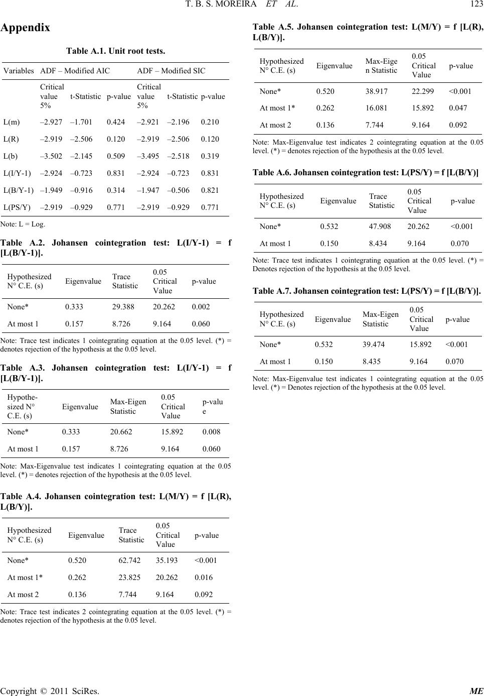

T. B. S. MOREIRA ET AL.
123
Appendix
Table A.1. Unit root tests.
Variables ADF – Modified AIC ADF – Modified SIC
Critical value
5% t-Statistic p-value Critical
value
5% t-Statistic
p-value
L(m) –2.927 –1.701 0.424 –2.921 –2.196 0.210
L(R) –2.919 –2.506 0.120 –2.919 –2.506 0.120
L(b) –3.502 –2.145 0.509 –3.495 –2.518 0.319
L(I/Y-1) –2.924 –0.723 0.831 –2.924 –0.723 0.831
L(B/Y-1) –1.949 –0.916 0.314 –1.947 –0.506 0.821
L(PS/Y) –2.919 –0.929 0.771 –2.919 –0.929 0.771
Note: L = Log.
Table A.2. Johansen cointegration test: L(I/Y-1) = f
[L(B/Y-1)].
Hypothesized
N° C.E. (s) Eigenvalue Trace Statistic
0.05
Critical
Value p-value
None* 0.333 29.388 20.262 0.002
At most 1 0.157 8.726 9.164 0.060
Note: Trace test indicates 1 cointegrating equation at the 0.05 level. (*) =
denotes rejection of the hypothesis at the 0.05 level.
Table A.3. Johansen cointegration test: L(I/Y-1) = f
[L(B/Y-1)].
Hypothe-
sized N°
C.E. (s) Eigenvalue Ma x-Eigen
Statistic
0.05
Critical
Value
p-valu
e
None* 0.333 20.662 15.892 0.008
At most 1 0.157 8.726 9.164 0.060
Note: Max-Eigenvalue test indicates 1 cointegrating equation at the 0.05
level. (*) = denotes rejection of the hypothesis a t t he 0.05 level.
Table A.4. Johansen cointegration test: L(M/Y) = f [L(R),
L(B/Y)].
Hypothesized
N° C.E. (s) Eigenvalue Trace Statistic
0.05
Critical
Value p-value
None* 0.520 62.742 35.193 <0.001
At most 1* 0.262 23.825 20.262 0.016
At most 2 0.136 7.744 9.164 0.092
Note: Trace test indicates 2 cointegrating equation at the 0.05 level. (*) =
denotes rejection of the hypothesis at the 0.05 level.
Table A.5. Johansen cointegration test: L(M/Y) = f [L(R),
L(B/Y)].
Hypothesized
N° C.E. (s) Eigenvalue Max-Eige n Statistic
0.05
Critical
Value p-value
None* 0.520 38.917 22.299 <0.001
At most 1* 0.262 16.081 15.892 0.047
At most 2 0.136 7.744 9.164 0.092
Note: Max-Eigenvalue test indicates 2 cointegrating equation at the 0.05
level. (*) = denotes rejection of the hypothesis at the 0.05 level.
Table A.6. Johansen cointegration test: L(PS/Y) = f [L(B/Y)]
Hypothesized
N° C.E. (s) Eigenvalue Trace Statistic
0.05
Critical
Value p-value
None* 0.532 47.908 20.262 <0.001
At most 1 0.150 8.434 9.164 0.070
Note: Trace test indicates 1 cointegrating equation at the 0.05 level. (*) =
Denotes rejection of the hypothesis at the 0.05 level.
Table A.7. Johansen cointegration test: L(PS/Y) = f [L(B/Y)].
Hypothesized
N° C.E. (s) Eigenvalue Max-Eigen Statistic
0.05
Critical
Value p-value
None* 0.532 39.474 15.892 <0.001
At most 1 0.150 8.435 9.164 0.070
Note: Max-Eigenvalue test indicates 1 cointegrating equation at the 0.05
level. (*) = Denotes reje ction of the hy pot hesis at the 0.05 level .