 Journal of Modern Physics, 2011, 2, 421-430 doi:10.4236/jmp.2011.25052 Published Online May 2011 (http://www.SciRP.org/journal/jmp) Copyright © 2011 SciRes. JMP A Scheme for Calculating Atomic Structures beyond the Spherical Approximation Mitiyasu Miyasita1, Katsuhiko Higuchi2, Masahiko Hig uchi3 1Graduate S chool of S cience an d E ngineering, Shinshu Un i versi t y, Ueda, Japan 2Graduate Sch ool of Advanced Science of M at te r , Hiros hi ma University, Higashi-Hiroshima, Japan 3Department of Physics, Faculty of Science, Shinshu University, Matsumoto, Japan E-mail: miyasita.mitiyasu@gmail.com Received February 11, 2011; revised April 3, 2011; April 4, 2011 Abstract We present a scheme for calculating atomic single-particle wave functions and spectra with taking into ac- count the nonspherical effect explicitly. The actual calculation is also performed for the neutral carbon atom within the Hartree-Fock-Slater approximation. As compared with the conventional atomic structure of the spherical approximation, the degenerate energy levels are split partially. The ground state values of the total orbital and spin angular momenta are estimated to be both about unity, which corresponds to the term 3P in the LS-multiplet theory. This means that the nonspherical effect may play an essential role in the description of the magnetization caused by the orbital polarization. Keywords: Nonspherical Distribution of Electrons, Spherical Approximation, Orbital Polarization, Atomic Structure, Carbon Atom 1. Introduction Let us start with revisiting the conventional atomic structures. We consider the isolated neutral atom with the atomic number . Neglecting the relativistic effects, the Schrödinger Equation for the stationary state is given by ˆ E (1) with 2 1, 21 2 ˆ 2 ZZ i iij iij ij Z Hr rr , (2) where i r and i r stand for the position of the ith elec- tron and its magnitude, respectively, and where the atomic unit is used. Equation (1) can be numerically solved only in small atomic systems, but in larger atomic systems we have to utilize the theories to reduce Equa- tion (1) into the effective single-particle Equation such as the Hartree [1], Hartre-Fock [2] and Kohn-Sham [3,4] Equations, etc. The single-particle Equation is generally written by 2ii ii V rr r , (3) where denotes the up-spin or down-spin . In order to solve Equation (3), we have usually used the spherical approximation, i.e., the central field approxi- mation [5]. Under such the approximation, Equation (3) is separable into two Equations, one of which depends on the radial variable r and the other on the angular vari- ables, and . If the effective potential is spherically symmetric and local [6], and if the solutions are given by 1, nlmnl lm prY r r, (4) then two Equations are 2 0 22 1 d dnlnl nl ll Vrprpr rr , (5) 2 ˆ,1, lm lm YllY l, (6) where ˆ l is the operator of the orbital angular momen- tum, and , lm Y are the spherical harmonics [7]. Radial wave functions nl pr of Equation (5) are cal- culated easily by means of the numerical methods such as the Herman-Skillman method [8,9]. Thus, the conven- tional atomic structures, where the eigenstates are speci- fied by the quantum numbers ,1,nlnmlm l and can be obtained. Here the question is raised of whether the spherical  M. MIYASITA ET AL. Copyright © 2011 SciRes. JMP 422 approximation is always appropriate or not. The spheri- cal approximation is reasonable for atoms having the outermost shell that is fully or half occupied since their electron densities are exactly spherical. However, in the other atoms the electron densities are not necessarily spherical, so that the conventional picture of the atomic structures is not rigorous but just an approximation. To what extent the effect of the nonspherical distribution of electrons (which is hereafter called the nonspherical ef- fect) modifies the conventional picture of the atomic structures seems to be interesting and important. This is because the electronic structures of molecules and solids have been frequently considered on the basis of the or- dinary atomic wave functions and spectra. The typical examples are the Slater integrals contained in the model Hamiltonians like the Hubbard model [10,11], and in the LDA + U method [12,13]. In addition to the above, there exists an obvious flaw in the spherical approximation. The total orbital angular momentum becomes necessarily zero in the conventional atomic structure, because the spherical approximation coincides with the filling approximation in which elec- trons are uniformly distributed into each state in the out- ermost shell [14]. This means that the orbital polarization never appears in the atomic structures of the spherical approximation. The orbital polarization is an origin of the magnetism of solids as well as the spin polarization [15-20], especially for the 5f-electron systems [15-17]. So far the orbital polarization has been discussed as a part of the correlation effects [17] or on the basis of the LS-multiplet theory [21]. In this paper, we shall discuss the nonspherical effect on the orbital polarization from the viewpoint of the single-particle picture. It will be shown in the following sections that the orbital polariza- tion appears without the correlation effects. As a first attempt to take into account the nonspherical effect, Slater has proposed a scheme for expanding the eigenfunctions of Equation (3) with the spherical har- monics [9]. However his method is difficult to be per- formed because an infinite number of simultaneous equations have to be solved. After Slater’s proposal, there have been two kinds of approaches to this problem. One is the variational method where the single-particle wave function is expanded by using appropriately chosen basis functions [22,23]. Another is the density functional scheme containing the effect of the orbital current den- sity explicitly.[24-31] In this paper, we adopt the former approach. As the basis functions, eigenfunctions for the spherical part of the single-particle potential are used and updated for each iteration of the self-consistent calcula- tions. They are apparently different from those of the previous works [22,23]. The aim of this paper is to present the tractable scheme for calculating the atomic structures beyond the spherical approximation, and to discuss the nonspherical effect. Organization of this paper is as follows. In Sec- tion 2, we present a scheme for dealing with the non- spherical effect explicitly. In order to check the validity of the scheme, we apply it to the neutral carbon atom in Section 3. The calculation procedure is also explained. The results are shown in Section 4, with a focus on the differences between the present atomic structures and the conventional one. The ground state values of the total orbital and spin angular momenta are also estimated. Finally concluding remarks are given in Section 5. 2. A Variational Method beyond the Spherical Approximation In this section, we present a variational method for cal- culating atomic structures with taking into account the nonspherical effect. Let us consider solving the single-particle Equation (3). The Hartree-Fock-Slater approximation is utilized [32], i.e., the effective potential of Equation (3) is given in a local form V r. First, we expand the effective poten- tial with the spherical harmonics: ** ,, lm lmlmlm lm VvrYvrY r, (7) where lm vr are the radial components and their ex- plicit forms are given in Appendix. For the convenience of the subsequent discussion, the operator of the left- hand side (LHS) of Equation (5) is defined as 22 022 ˆ d ˆ:d Vr rr l, (8) where let Vr be the spherically averaged potential for Equation (7), which is defined as * 00 00 1()sind d 4π 1. 4π Vr V vrvr r (9) In the Expansion 7, the term 00lm corresponds to the spherical part of the effective potential as shown in Equation (9), while the other terms correspond to the nonspherical parts. Next, in a similar way to Equation (7), we shall ex- pand the solution of Equation (3) with the set of known functions. As the known functions, we here adopt ones given by Equation (4), the radial part of which is the ei- genfunction for the Hamiltonian 8. Thus, the solution of Equation (3) is written as , 1, i inllmnllm nll m CprY r r. (10)  M. MIYASITA ET AL. Copyright © 2011 SciRes. JMP 423 Substituting Equations (7) and (10) into Equation (3), and writing distinctly the spherical and nonspherical parts of the effective potential, we get 0 (00) ** ˆ,(), ,, ,, i NL NLLL NL L i LL NLNL NL i iNLNL NL HCprY vrY vrY CprY Cp rY (11) where we use Equations (8) and (9), and abbreviate nl as “N” and lm as “L” for ease of seeing. It can be easily shown that Equation (11) is reduced to the spherical Equation including Equation (5), if the second term of the LHS is neglected. This means that the second term of the LHS represents the nonspherical effect that has been disregarded in the conventional spherical approximation. Here, for simplicity, we shall use the common value of l for N and L, and suppose that the eigenvalues for the Hamiltonian 8 is denoted as 0 . Multiplying 11 ** 1, NL prY r on both sides of Equation (11) and integrating over the whole space, we have 1 11 11 00 * 2 d0 NN LL NNi NL i NLLN NL O prVrprrC , (12) where 11 *d, NN NN Oprprr (13) 1 1 1 * (00) *** (00) () ,,,sindd ,,,sindd. LL LLL L L LLL L L Vr vrYY Y vr YYY (14) Equation (12) is just the generalized eigenvalue prob- lem. If the matrix elements, 1 N O and 1 NN Vr , and the energy spectra of the spherical approximation, 0 , are given, then we can obtain the eigenvalues, i , and eigenfunctions, i L C . It should be noted that the ei- genvalues i are guaranteed to be real since both ma- trices of Equation (12) are hermitian. The angular inte- grations in Equation (14) can be analytically calculated by using the Wigner 3j-symbols. According to the prop- erties of the Wigner 3j-symbols, matrix elements of Equation (14) are zero unless 1evenlll , 11 lllll and 1 mm m [7]. These condi- tions also determines the upper limit of the summation of Equation (7). The eigenfunctions thus obtained yield the new poten- tials by means of the expressions given in Appendix. These potentials should coincide with the input ones. Namely, the self-consistency is required for the poten- tials. The corresponding basis functions in Equation (10) are modified for each iteration since the function nl pr is the radial part of solution for the Hamiltonian (8) with the Potential 9. The iteration is continued until self-con- sistency for the potentials is achieved. Let us show the detailed procedure of the self-consis- tent calculations. The flow chart of self-consistent calcu- lations is shown in Figure 1. We first give a starting po- tential in some way, for example via the LDA calculation within the spherical approximation (Step 1 in Figure 1). In order to prepare the radial basis functions nl pr , the spherical parts of the potential are derived. Using these potentials, atomic structure calculations are performed (Step2). Then, using the basis functions and correspond- ing spectra, the generalized eigenvalue problem is solved (Step3). The resultant eigenfunctions provide the new potentials (Step 4). Here we check whether the potentials are converged or not (Step 5). Of course, the checking should be performed on both convergences for the spheri- cal and nonspherical parts of potentials. If the conver- gence is not yet obtained, we return to Step 2 with the spherical potential calculated from the new potential. The calculations are repeated until the potentials are con- verged within some accuracy. 3. Application to the Neutral Carbon Atom Compared to the previous ones [9,22,23], the present scheme seems to be more tractable, but as to the effec- tiveness actual calculations have to be performed. Here we apply it to the neutral carbon atom. In the Expansion 10, we choose the common value of l in both summations for nl and lm . That is to say, physically meaningful functions are prepared for basis functions of the expansion. In more detail, we use five functions having the following quantum numbers: 100,200,211,210,21 1nlm . Correspondingly, the upper limit of the potential given by Equation (7) is determined from the properties of the Wigner 3j symbols, as already mentioned below Equa- tion (15). This time, the expansion of the potential con- sists of the following terms: ()00, 11,10,11 ,22, 21,20,2 1,22 lm . The generalized eigenvalue problem is reduced to 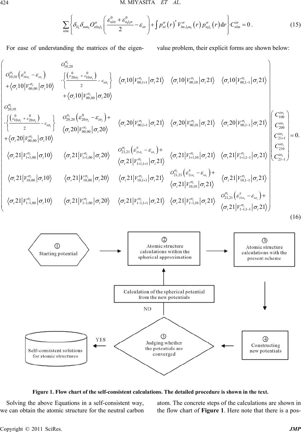 M. MIYASITA ET AL. Copyright © 2011 SciRes. JMP 424 11 11111 111 00 * ,d0 2 nln li llmmnlnlinllml mnlnlm nlm OprVrprrC . (15) For ease of understanding the matrices of the eigen-value problem, their explicit forms are shown below: 0 10 10,20 00 10,10 20 10 00,1 100,1000,11 00,00 00,00 20,10 00 20,20 20 10 20 00,00 2 2 1021 1021 1021 10 10 10 20 20 10 ii i iiii iii i i i i i ii i i iii ii ii ii ii i ii O O O O VVV V V V 0 21 0 00,1 100,1000,11 00,00 21,21 11,0011,0011,1011,11 11,11 10,00 2021 20212021 20 20 211021202121 2121 21 21 21 102 ii ii iii i ii ii ii i i i iiiiii ii iiiiiii i ii ii i O VVV V VV VV V V 0 21 0 21 21,21 10,0010,1 110,11 10,10 21,21 11,0011,0011,11 11,10 11,11 12021 212121 21 21 211021202121 2121 21 21 ii ii ii ii i i ii iiii i ii ii i ii iiiii iii ii O O VV V VVVV V V 100 200 211 210 21 1 0. i i i i i i i i i i C C C C C (16) Figure 1. Flow chart of the self-consistent calculations. The detailed procedure is shown in the text. Solving the above Equations in a self-consistent way, we can obtain the atomic structure for the neutral carbon atom. The concrete steps of the calculations are shown in the flow chart of Figure 1. Here note that there is a pos-  M. MIYASITA ET AL. Copyright © 2011 SciRes. JMP 425 sibility to exist the multiple self-consistent solutions. In order to cover such solutions, various kinds of input po- tentials should be arranged. This time, we prepare the orbitals of the spherical approximations, i.e. 1s, 2s and 2p orbitals, and take the linear combination of them so as to construct the input potentials. The 1s and 2s orbitals are used as they stand, while 2p orbitals are transformed into the following orbitals: 1 2 3 211 210 21 1 cos sin0 sincos 0 001 cos0 sin 010 sin0cos , (17) where 21121021 1 , and are 2p orbitals of the spheri- cal approximation. The input potentials are constructed from the 1s, 2s and two orbitals chosen among three ones given by Equation (17). The angles and are changed by 15°, respectively. A total of 864 kinds of different potentials are taken as the starting potentials ( 32 360 1518015864C ). As shown in a subsequent section, six kinds of self-consistent solutions can be ob- tained correspondingly to the starting potentials. 4. Results and Discussions In this section, we will give the results of the atomic structure of the neutral carbon atom. Figure 2 shows the energy spectra of the present scheme, together with those of the conventional spherical approximation. It should be noted that the conventional atomic spectra can be speci- fied by the quantum numbers nlm , but in the present scheme they are specified only by the ordinal numbers because of lack of the spherical symmetry. For instance, 1s states of the spherical approximation correspond to the 1st and 2nd states of the present scheme. The conventional 2p states are split into doubly de- generate levels and single one due to the nonspherical effect. There exist two types of splitting. In other words, two types of the converged self-consistent solutions (SCS) can be found from the viewpoint of the splitting of energy levels. One is that the doubly degenerate levels are higher than the single one, and another is the opposite. They are denoted as “SCS-A” and “SCS-B”, respectively, in Figure 2. On the other hand, conventional 1s and 2s states are little influenced by the nonspherical effect. This is because the 2p states (5th and 6th states) are di- rectly influenced by their nonspherical densities of elec- trons, while the wave functions for 1s and 2s states (from 1st to 4th states) are well localized near the nuclear where the spherical potential mainly caused by the nu- clear is dominant. In order to discuss the ground-state properties in more detail, we shall investigate the components of the eigen- functions, i.e. the expansion coefficients of Equation (10). The SCS-A and SCS-B are classified into two and four types, respectively, according to the components of the Figure 2. Energy spectra for the neutral carbon atom. The first column shows the results for the conventional spherical ap- proximation. The second and third columns are the self-consistent solutions for the present scheme, which are denoted as “SCS-A” and “SCS-B”, respectively. The up- and down-arrows denote the occupied states, and open circle the unoccupied states. All values are given in Rydberg Unit.  M. MIYASITA ET AL. Copyright © 2011 SciRes. JMP 426 wave function. They are denoted as A-1, A-2 and B-1, B-2, B-3, B-4 respectively. The expansion coefficients for the 1st, 2nd, 3rd and 4th states are shown in Table 1. For all of the coverged SCSs, the components are same as those of the spherical approximation within the accu- racy of 3 10. These results are consistent with the fact that the states from 1st to 4th for the present scheme are in a good agreement with the conventional 1s and 2s states, respectively (Figure 1). Concerning the 5th and 6th states, there is a large difference between the present and conventional schemes, which is shown in Table 2. In the conventional spherical approximation, electrons are distributed into each shell in an equal weight, so that the corresponding coefficients are all 23. Meanwhile, components of each the converged SCS are partial to some of them. This partiality causes the polarization of the orbital angular momenta, which is so-called orbital polarization. In order to verify it, we calculate the ground state values of the total orbital and spin angular momenta. The ground state of the Hartree-Fock-Slater approxima- tion is given by a single Slater determinant that is writ- ten as 11 141 1 111 211 14 444 4 16 15515 525 5 166166266 1 ,, 6! xx rrrr rr rrr rrr (18) where i denote the coordinates for ith electron in- cluding spatial coordinate i r and spin coordinate i , and where () i r is the solution of Equation (16), and where () and () are wave functions for up- and down-spins, respectively. Using Equation (18), the total orbital angular momentum and its z-component, L and L, are respectively calculated by 2 16 16 ˆ (, ),1xxxx LLL, (19) 16 16 ˆ ,, z xLx xL, (20) where 6 1 ˆ ˆi i l, and ˆ i l is the operator of the orbital angular momentum for the ith electron. Similarly, the total spin angular momentum and its z-component, S and S, are respectively given by 2 16 16 ˆ ,,1xxxx SS S, (21) 16 16 ˆ ,, z xSx xS , (22) where 6 1 ˆˆi i s, and ˆi s is the operator of the spin an- gular momentum for the ith electron. The results are shown in Table 3. In a nonrelativistic many-electron system, ,, and z LL SS are the conserved quantities. All of the coverged SCSs yield 1 and 1LS within the ac- curacy of 3 10 . This means that the ground states of the present scheme correspond to the term 3P that is known to be the ground state of the LS-multiplet theory. Fur- thermore, it is noticed that the present scheme obviously Table 1. The expansion coefficients of Equation (10) for the 1st, 2nd, 3rd and 4th states. Both SCS-A and SCS-B give the same results, so we don’t lable SCS-A and SCS-B distinctly. (nlm) Energy [Ryd.] (100) (200) (21+1) (210) (21-1) –21.354 1.000 … … … … –21.206 1.000 … … … … –1.421 … 1.000 … … … Spheical approximation –1.032 … 1.000 … … … –21.353 1.000 0.000 0.000 0.000 0.000 –21.206 1.000 0.000 0.000 0.000 0.000 –1.421 0.000 1.000 0.000 0.000 0.000 Present results for SCS-A and SCS-B –1.031 0.000 1.000 0.000 0.000 0.000  M. MIYASITA ET AL. Copyright © 2011 SciRes. JMP 427 Table 2. The expansion coefficients of Equation (10) for the 5th and 6th states. (nlm) Energy [Ryd.] (100) (200) (21+1) (210)(21-1) Spheical approximation –0.782 … … 23 23 23 –0.799 0.000 0.000 0.000 1.0000.000 SCS A-1 –0.773 0.000 0.000 1.000 0.0000.000 –0.799 0.000 0.000 0.000 1.0000.000 SCS A-2 –0.733 0.000 0.000 0.000 0.0001.000 –0.799 0.000 0.000 12 0.000 12 SCS B-1 –0.799 0.000 0.000 12 0.000 12 –0.799 0.000 0.000 1.000 0.0000.000 SCS B-2 –0.799 0.000 0.000 0.000 0.0001.000 –0.799 0.000 0.000 0.000 1.0000.000 SCS C-1 –0.799 0.000 0.000 12 0.000 12 –0.799 0.000 0.000 0.000 1.0000.000 SCS C-2 –0.799 0.000 0.000 12 0.000 12 Table 3. The ground state values of the tptal orbital angular momentum and itd z-component, L and LZ, are showm in the 1st and 2nd cplumns. Also, the ground state values of the total spin angular momentum and its z-component, S and SZ, are shown in the 3rd and 4th columns. State L LZ S SZ SCS A-1 1.000 1.000 1.000 1.000 SCS A-2 1.000 –1.000 1.000 1.000 SCS B-1 1.000 0.000 1.000 1.000 SCS B-2 1.000 0.000 1.000 1.000 SCS B-3 1.000 0.000 1.000 1.000 SCS B-4 1.000 0.000 1.000 1.000 causes the orbital polarization. Since the spherical ap- proximation never brings it, we may say that the non- spherical effect is one of the keys to the appearance of the orbital polarization. Here note that the SCSs are classified into three kinds of states, which yield 1,0 and 1 z L, respectively. This is not surprising because the term 3P are triply de- generate with respect to the orbital angular momentum. These three states, by their nature, should be completely degenerate and their total energies should be same as each other. Actually, the total energies of these states which are also evaluated by taking the expectation values of the Hamiltonian with respect to Equation (18) coin- cide with each other. 5. Concluding Remarks In this paper, we present a scheme for calculating the atomic structures beyond the spherical approximation and investigate to what extent the single-particle picture of atomic systems needs to be modified. It is confirmed that the orbital polarization can appear only by consider- ing the nonspherical effect explicitly. Compared to the conventional atomic structures, we find that the atomic levels are partially split. The magnitude of splitting for 2p states is about 5%, which is never neglected because the splitting itself causes the orbital polarization. Also, such a debacle of the conventional atomic structures seems to be conceptually important. Although the present scheme shows the necessity of modifying the single-particle picture of atomic systems, we have to consider the following effects that are ne- glected in the present calculations: 1) enhancement of the expansion basis functions in Equation (10); 2) treatment of the exchange energy beyond the Har- tree-Fock-Slater approximation; 3) correlation effects. Concerning the first effect, we here adopt only 1s, 2s and 2p orbitals in the expansion of the eigenfunctions. However we had better take more functions as the basis functions. Especially for the neutral carbon atom, 3d orbitals should be added to the expansion basis functions since the nondiagonal elements between the 2p and 3d states would not be negligibly small in Equation (12) or (15). Similarly, the second and third effects seem to be indispensable for describing the nonspherical effect in more detail. But anyway, we can say within the knowl- edge obtained in this paper that the orbital polarization certainly emerges by taking into account the nonspheri- cal effect even if the correlation effects are not explicitly considered. Furthermore, the effect of the nonspherical distribution of electrons cannot be neglected not only conceptually but also quantitatively in the study on the single-particle picture of atomic systems. 6. Acknowledgements This work was partially supported by Grant-in-Aid for Scientific Research (No. 19540399) and for Scientific Research in Priority Areas (No. 17064006) of The Min- istry of Education, Culture, Sports, Science, and Tech- nology, Japan.  M. MIYASITA ET AL. Copyright © 2011 SciRes. JMP 428 7. Reference [1] D. R. Hartree, “The Wave Mechanics of an Atom with a Noncoulomb Central Field. PartI: Theory and Method. Part II: Some Results and Discussions,” Proceedings of Cambridge Philosophical Society, Vol. 24, No. 1, 1928, 111-132. [2] V. Fock, Z. Physik, “Näherungsmethode zur Lösung des quantenmechanischen Mehrkörperproblems,” Zeitschrift Für Physik, Vol. 61, No. 1-2, pp. 126-148. doi:10.1007/BF01340294 [3] P. Hohenberg and W. Kohn, “Inhomogeneous Electron Gas,” Physical Review, Vol. 136, No. 3B, 1964, pp. 864-871. doi:10.1103/PhysRev.136.B864 [4] W. Kohn and L. J. Sham, “Self-Consistent Equations Including Exchange and Correlation Effects,” Physical Review, Vol. 140, No. 4A, 1965, pp. 1133-1138. doi:10.1103/PhysRev.140.A1133 [5] The spherical approximation means that the effective potential in Equation (3) is approximated into the central field, i.e., ii VVr . For instance, see, J. C. Slater, “Quantum Theory of Atomic Structure,” McGraw-Hill, NY, Vol. 1, 1960. [6] This means that i VVr . [7] A. Messiah, “Quantum Mechanics”, Dover Publications, NY, 1999. [8] F. Herman and S. Skillman, “Atomic Structure Calcula- tions,” Prentice-Hall Inc., New Jersey, 1963. [9] J. C. Slater, “The Calculation of Molecular Orbitals,” John Wiley & Sons, NY, 1979. [10] N. F. Mott, “The Basis of the Electron Theory of Metals, with Special Reference to the Transition Metals,” Pro- ceedings of the Physical Society, London, Section A, Vol. 62, No. 7, 1949, p. 416. doi: 10.1088/0370-1298/62/7/303 [11] P. W. Anderson, “New Approach to the Theory of Su- perexchange Interactions,” Physical Review, Vol. 115, No. 1, 1959, pp. 2-13. doi: 10.1103/PhysRev.115.2 [12] V. I. Anisimov, J. Zaanen and O. K. Andersen, “Band Theory and Mott Insulators: Hubbard U instead of Stoner,” Physical Review B, Vol. 44, No. 3, 1991, pp. 943-954. doi:10.1103/PhysRevB.44.943 [13] A. I. Liechtenstein, V. I. Anisimov and J. Zaanen, “Den- sity-Functional Theory and Strong Interations: Orbital Ordering in Mott-Hubbard Insulators,” Physical Review B, Vol. 52, No. 8, 1995, R5468-R5470. [14] S. E. Koonin, “Computational Physics,” Addison-Wesley, NY, 1986. [15] O. Eriksson, B. Johansson, R. C. Albers, A. M. Boring and M. S. S. Brooks, “Orbital magnetism in Fe, Co, and Ni,” Physical Review B, Vol. 42, 1990, 2707-2710. doi:10.1103/PhysRevB.42.2707 [16] O. Eriksson, M. S. S. Brooks and B. Johansson, Phys. Rev. B 41, 7311 (1990). doi: 10.1103/PhysRevB.42.2707 [17] M. S. S. Brooks, O. Eriksson, L. Severin and B. Johans- son, “Spin and Orbital Magnetization Densities in Itiner- ant Magnets” Physica B, Vol. 192, No. 1-2, 1993, pp. 39-49. doi:10.1016/0921-4526(93)90106-G [18] T. Shishidou, T. Oguchi and T. Jo, “Hartree-Fock Study on the 5f Orbital Magnetic Moment of US,” Physical Re- view B, Vol. 59, No. 10, 1999, pp. 6813-6823. doi:10.1103/PhysRevB.59.6813 [19] M. R. Norman, “Orbital polarization and the insulating gap in the transition-metal oxides,” Physical Review Let- ters, Vol. 64, No. 10, 1990, pp. 1162-1165. doi:10.1103/PhysRevLett.64.1162 [20] G. H. Daalderop, P. J. Kelly and M. F. H. Schuurmans, “Magnetocrystalline Anisotropy and Orbital Moments in Transition-Metal Compounds,” Physical Review B, Vol. 44, No. 21, 1992, pp. 12054-12057. doi:10.1103/PhysRevB.44.12054 [21] A. Narita and M. Higuchi, “Expressions of Energy and Potential due to Orbital Polarization,” Journal of the Physical Society of Japan, Vol. 75, No. 2, 2006, pp. 024301-024301-10. doi:10.1143/JPSJ.75.024301 [22] J. F. Janak and A. R. Williams, “Method for Calculating Wave Functions in a Nonspherical Potential,” Physical Review B, Vol. 23, No. 12, 1981, pp. 6301-6306. doi:10.1103/PhysRevB.23.6301 [23] F. W. Kutzler and G. S. Painter, “Energies of Atoms with Nonspherical Charge Densities Calculated with Nonlocal Density-Functional Theory,” Physical Review Letters, Vol. 59, No. 12, 1987, 1285-1288. doi:10.1103/PhysRevLett.59.1285 [24] A. D. Becke, “Local Exchange-Correlation Approxima- tions and First-Row Molecular Dissociation Energies,” International Journal of Quantum Chemistry, Vol. 27, No. 5, 1985, pp. 585-594. doi:10.1002/qua.560270507 [25] A. D. Becke, “Current Density in Exchange-Correlation Functionals: Application to Atomic States,” Journal of Chemical Physics, Vol. 117, No. 15, 2002, pp. 6935-6938. doi:10.1063/1.1503772 [26] E. Orestes, T. Marcasso and K. Capelle, “Den- sity-Functional Calculation of Ionization Energies of Cur- rent-Carrying Atomic States,” Physical Review A, Vol. 68, No. 2, 2003, 022105. doi:10.1103/PhysRevA.68.022105 [27] E. Orestes, A. B. F. da Silva and K. Capelle, “Energy Lowering of Current-Carrying Single-Particle States in Open-Shell atoms due to an Exchange-Correlation Vector Potential,” International Journal Of Quantum Chemistry, Vol. 103, No. 5, 2005, pp. 516-522. doi:10.1002/qua.20575 [28] G. Vignale and M. Rasolt, “Density-Functional Theory in Strong Magnetic Fields,” Physical Review Letters, Vol. 59, No. 20, 1987, pp. 2360-2363. doi:10.1103/PhysRevLett.59.2360 [29] G. Vignale and M. Rasolt, “Current- and Spin-Density- Functional Theory for Inhomogeneous Electronic Sys- tems in Strong Magnetic Fields,” Physical Review B, Vol. 37, No. 18, 1988, 10685-10696. doi:10.1103/PhysRevB.37.10685 [30] M. Higuchi and A. Hasegawa, “A Relativistic Current-  M. MIYASITA ET AL. Copyright © 2011 SciRes. JMP 429 and Spin-Density Functional Theory and a Single-Particle Equation,” Journal of the Physical Society of Japan, Vol. 66, No. 1, 1997, p. 149 (1997). doi:10.1143/JPSJ.66.149 [31] M. Higuchi and A. Hasegawa, “Single-Particle Equation of Relativistic Current- and Spin-Density Functional Theory and Its Application to the Atomic Structure of the Lanthanide Series,” Journal of the Physical Society of Japan, Vol. 67, No. 6, 1998, pp. 2037-2047. doi:10.1143/JPSJ.67.2037 [32] J. C. Slater, “A Simplification of the Hartree-Fock Method,” Physical Review, Vol. 81, No. 3, 1951, pp. 385-390.doi: 10.1103/PhysRev.81.385 Appendix Expressions for the Potentials In this appendix, we present the expressions for the spherical and nonspherical parts of the effective potential. The effective potential consists of three terms, i.e., the nuclear, Hartree and exchange potentials, which are given by 1 1 3 3 23 2d6, 4π Z Vr r rrr rr (A1) where the exchange potential is simplified with the aid of the Slater approximation [32], and where r and r denote the electron density and electron density with -spin, respectively. Using Equation 10, they are written as occ. 2 2 occ. , 2 1,, i i i nll mnllm inllm CprY r rr (A2) OCC OCC .2 spin 2 . , 2 spin 1(), , i i i nll mnllm inllm CprY r rr (A3) where the sum of Equation A3 is over only the occupied states with -spin. What we need are 1) spherical part of Equation A1, i.e., Vr * 00 00 1 4πvrvr , that appears in Equation 8, and 2) nonspherical components of Equation A1, i.e., kq vr , that appear in Equation 12 or 14. The above 1) is indispensable for deriving the basis functions nl pr and corresponding spectra 0 nl , which are also used in Equation 12 or 14. Now let us show the explicit forms of 1) and 2) by considering each term of Equation A1. As for the first term, we have no problem because it is exactly spherical. Also, the second term can be easily separated into the spherical and nonspherical parts by means of the multi- pole expansion of the Coulomb potential. Concerning the third term, we have to use an approximation so as to de- rive one third power of r. Using the composition relation for the spherical harmonics, r is formally separated into spherical and nonspherical parts as fol- lows: SNS r rr, (A4) with 2 OCC 112 2112 21111 11 2 2112 2 .* * ,, 22 2 spin 22 22 22 1 12121 8 0 0.., 0 000 m Sii nllmnllmnlnl inllmnllm rCCprprll r ll ll CC mm (A5) and OCC OCC 112 21122 11 2 21122 222 11 11 22 .. 2* ,, 2 spin spin 1 2 22 * 0 0 22 22 2 1 () () 1212121 ()()24π 000 NSi i inllm nllm iinll mnllm mll k nl nlkl lqk CC r llk prpr llk llk m rr 2 (, )... kq YCC mq (A6)  M. MIYASITA ET AL. Copyright © 2011 SciRes. JMP Since NS r is constructed from electrons of the unfilled outermost shell alone, it is quite smaller than the spherical part of the electron density. That is to say, SNS r r. Using this fact, we can get an ap- proximate form of the one third power of r as follows 11 2 33 3 1 3 SSNS rr rr, (A7) The first and second terms turn to the spherical and nonspherical parts of the exchange potential, respectively. Using these relations, the resultant forms of 1) and 2) are, respectively, given by 1122 11221111 11 2211 22 2 occ. * * ,, 1 1 3 22 22 3 22 22 21 d 0 03 2121216, 0 000 4 ii nllmnllmnlnl i nllmnllm mS Z VrCCrp rp r rr ll ll ll r mm (A8) 11 2211 221111 11 2 2112 2 2 11 22122 occ. * * ,, 1 22 22 22 22 1 2 3* 3,, 2 d 4π2121 1000 21 31 24π k ii kqnllmnllmnlnl k inllmnllm m Sii nllmnlm r vCCrprpr r llk llk ll mmq k rCC r r OCC 11 1 11 22122 2 .* ( spin) 1 222 22 22 22 1(21)2121 . 000 24π nl nl inllmnllm m prpr llk llk llk mmq (A9) Here 123 123 lll mmm is the Wigner 3j symbol [7], and Sr is given by Equation A5.
|