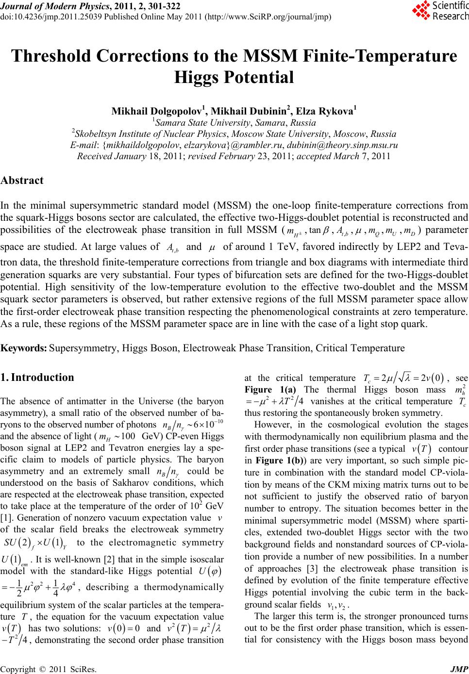
 Journal of Modern Physics, 2011, 2, 301-322 doi:10.4236/jmp.2011.25039 Published Online May 2011 (http://www.SciRP.org/journal/jmp) Copyright © 2011 SciRes. JMP Threshold Corrections to the MSSM Finite-Temperature Higgs Potential Mikhail Dolgopolov1, Mikhail Dubinin2, Elza Rykova1 1Samara State University, Samara, Russia 2Skobeltsyn Institute of Nuclear Physics, Moscow State University, Moscow, Russia E-mail: {mikhaildolgopolov, elzarykova}@rambler.ru, dubinin@theory.sinp.msu.ru Received January 18, 2011; revised February 23, 2011; accepted March 7, 2011 Abstract In the minimal supersymmetric standard model (MSSM) the one-loop finite-temperature corrections from the squark-Higgs bosons sector are calculated, the effective two-Higgs-doublet potential is reconstructed and possibilities of the electroweak phase transition in full MSSM ( m ,tan ,,tb , ,Q m,U m, m) parameter space are studied. At large values of ,tb and of around 1 TeV, favored indirectly by LEP2 and Teva- tron data, the threshold finite-temperature corrections from triangle and box diagrams with intermediate third generation squarks are very substantial. Four types of bifurcation sets are defined for the two-Higgs-doublet potential. High sensitivity of the low-temperature evolution to the effective two-doublet and the MSSM squark sector parameters is observed, but rather extensive regions of the full MSSM parameter space allow the first-order electroweak phase transition respecting the phenomenological constraints at zero temperature. As a rule, these regions of the MSSM parameter space are in line with the case of a light stop quark. Keywords: Supersymmetry, Higgs Boson, Electroweak Phase Transition, Critical Temperature 1. Introduction The absence of antimatter in the Universe (the baryon asymmetry), a small ratio of the observed number of ba- ryons to the observed number of photons 10 610 B nn and the absence of light (100 H m GeV) CP-even Higgs boson signal at LEP2 and Tevatron energies lay a spe- cific claim to models of particle physics. The baryon asymmetry and an extremely small B nn could be understood on the basis of Sakharov conditions, which are respected at the electroweak phase transition, expected to take place at the temperature of the order of 102 GeV [1]. Generation of nonzero vacuum expectation value v of the scalar field breaks the electroweak symmetry 21 Y SU U to the electromagnetic symmetry 1em U. It is well-known [2] that in the simple isoscalar model with the standard-like Higgs potential U 22 4 11 24 , describing a thermodynamically equilibrium system of the scalar particles at the tempera- ture T, the equation for the vacuum expectation value vT has two solutions: 00v and 22 vT 24T, demonstrating the second order phase transition at the critical temperature 220 c Tv , see Figure 1(a) The thermal Higgs boson mass 2 h m 22 4T vanishes at the critical temperature c T thus restoring the spontaneously broken symmetry. However, in the cosmological evolution the stages with thermodynamically non equilibrium plasma and the first order phase transitions (see a typical vT contour in Figure 1(b)) are very important, so such simple pic- ture in combination with the standard model CP-viola- tion by means of the CKM mixing matrix turns out to be not sufficient to justify the observed ratio of baryon number to entropy. The situation becomes better in the minimal supersymmetric model (MSSM) where sparti- cles, extended two-doublet Higgs sector with the two background fields and nonstandard sources of CP-viola- tion provide a number of new possibilities. In a number of approaches [3] the electroweak phase transition is defined by evolution of the finite temperature effective Higgs potential involving the cubic term in the back- ground scalar fields 12 ,vv. The larger this term is, the stronger pronounced turns out to be the first order phase transition, which is essen- tial for consistency with the Higgs boson mass beyond  M. DOLGOPOLOV ET AL. Copyright © 2011 SciRes. JMP 302 (a) (b) Figure 1. Contours on the (v, T) plane for (a) the second order phase transition (fracture point) and (b) the first or- der phase transition at the critical temperature Tc . the LEP2 exclusion 115 GeV H m. Enhancement of the cubic term in the MSSM at the one-loop level is sub- stantial in the class of MSSM scenarios with a light right stop [4]. Temperature loop corrections from the stop and other additional scalar states could be large and lead to the first order phase transition, the intensity of the latter de- pends or cc vT T , where 22 12ccc vTvT vT is the vacuum expectation value at the critical tempera- ture c T. The electroweak baryogenesis could be ex- plained if 1 cc vT T [5], the case of strong first order phase transition. In a number of analyses the MSSM finite-temperature effective potential is taken in the representation 012 1 1 ,,,0 ,0 ()(), eff ring VvT VvvVmv VT VT (1) where 0 V is the tree-level MSSM two-doublet potential at the SUSY scale, 1 V is the (non-temperature) one- loop resumed Coleman-Weinberg term, dominated by stop and sbottom contributions, 1 VT is the one-loop temperature term and ring V is the correction of re- summed leading infrared contribution from multi-loop ring (or daisy) diagrams. The MSSM relations between the 21 Y SU U gauge couplings 2 and 1 , and the quartic parameters 1, 2,3 ,4 of the potential 01 2 (, ,0)Vvv are very restrictive. Only two additional parameters 21 tan vv and m (charged scalar mass) determine the zero-temperature two-doublet Higgs sector at tree- level. The one-loop radiative corrections, both logarith- mic and non-logarithmic generated at the threshold SUSY M, can change strongly the tree-level picture. They depend on the parameters (,tb , ,Q m,U m, m) of the scalar quarks-Higgs bosons interaction sector. In most cases for the analysis in the representation (1) numerical methods are used to find the critical temperature c T, for example, by solving the equation for the determinant of second derivatives of the potential (1) at 1,2 0v [6]. Then the two background fields 1,2 c vT are found at the minimum using the minimization conditions (i.e. the absence of linear terms of the effective potential repre- sentation in the “shifted” fields). The first order phase transition strength is dependent on the cubic term 3 ETv which appears from the infrared region. Numerical high-precision Monte Carlo simulations on the lattice [7] have been developed and applied to MSSM in connection with the infrared problem [8] inherent to all analyses based on the effective potentials. Infrared divergences appear in the integration over bosonic static (00 ) Matsubara modes, which in the loop expansion for the three-dimensional momentum space correspond to the intermediate massless bosons. The non-perturbat- ive investigations of the problem have been performed in the framework of high-temperature dimensional reduc- tion [9,10], when an effective three-dimensional MSSM with the same Green’s functions as in the four-dimen- sional MSSM for the light bosons is constructed [11-13] by integrating out perturbatively the non-static modes. Corrections from squarks and gauge bosons are intro- duced after the reduction to the three-dimensional model. In order to cover the temperature range from very low temperatures to temperatures of the order of critical, the following analysis uses an approach developed in [14,15] for the general (non-temperature) two-Higgs doublet potential with complex-valued parameters 2 12 , 5 , 6 and 7 , which violates the CP-invariance explicitly. However, in this publication a simplified situation of the Higgs potential in the CP conserving limit is considered (the imaginary parts of the effective parameters 5,6,7 and 2 12 are taken to be zero). Full MSSM effective potential in the generic 1 ,2 basis has the form 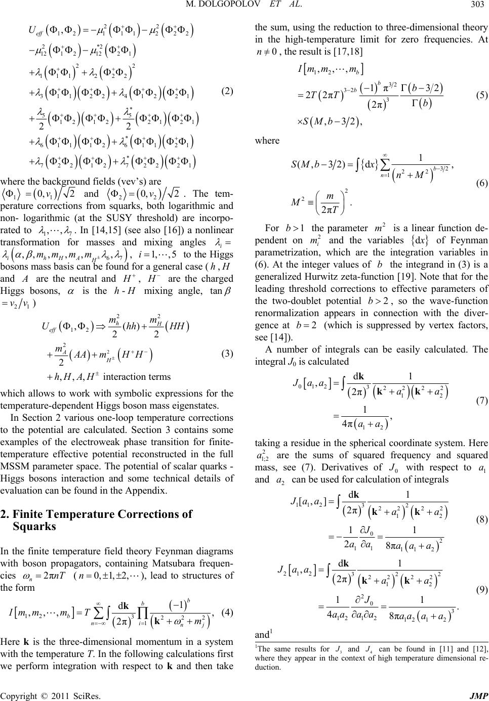 M. DOLGOPOLOV ET AL. Copyright © 2011 SciRes. JMP 303 22 121 112 22 2*2 1212122 1 22 1112 22 311 2241221 55 12 1221 21 * 61112611 21 * 722 1272221 , 22 eff U (2) where the background fields (vev’s) are 1 1 0, 2v and 22 0, 2v . The tem- perature corrections from squarks, both logarithmic and non- logarithmic (at the SUSY threshold) are incorpo- rated to 17 ,, . In [14,15] (see also [16]) a nonlinear transformation for masses and mixing angles i 67 ,, ,,,, ihHA H mm mm , 1,, 5i to the Higgs bosons mass basis can be found for a general case (h, and are the neutral and , are the charged Higgs bosons, is the h- mixing angle, tan 21 vv) 2 22 12 2 ,() 22 2 ,,, interaction terms hH eff A H mm UhhHH mAAmH H hH AH (3) which allows to work with symbolic expressions for the temperature-dependent Higgs boson mass eigenstates. In Section 2 various one-loop temperature corrections to the potential are calculated. Section 3 contains some examples of the electroweak phase transition for finite- temperature effective potential reconstructed in the full MSSM parameter space. The potential of scalar quarks - Higgs bosons interaction and some technical details of evaluation can be found in the Appendix. 2. Finite Temperature Corrections of Squarks In the finite temperature field theory Feynman diagrams with boson propagators, containing Matsubara frequen- cies 2π nnT (0, 1,2,n), lead to structures of the form 12 3222 1 1 d ,,,, 2π b b b ni nj ImmmTm k k (4) Here k is the three-dimensional momentum in a system with the temperature T. In the following calculations first we perform integration with respect to k and then take the sum, using the reduction to three-dimensional theory in the high-temperature limit for zero frequencies. At 0n , the result is [17,18] 12 32 32 3 ,,, 1π32 22π 2π ,32, b b b Imm m b TT b SMb (5) where 32 22 1 2 2 1 (, 32)d, . 2π b n SMb x nM m MT (6) For 1b the parameter 2 m is a linear function de- pendent on 2 i m and the variables d of Feynman parametrization, which are the integration variables in (6). At the integer values of b the integrand in (3) is a generalized Hurwitz zeta-function [19]. Note that for the leading threshold corrections to effective parameters of the two-doublet potential 2b, so the wave-function renormalization appears in connection with the diver- gence at 2b (which is suppressed by vertex factors, see [14]). A number of integrals can be easily calculated. The integral J0 is calculated 012 32222 12 12 d1 , 2π 1, 4π Jaa aa aa k kk (7) taking a residue in the spherical coordinate system. Here 2 1;2 a are the sums of squared frequency and squared mass, see (7). Derivatives of 0 with respect to 1 a and 2 a can be used for calculation of integrals 11 232 22 22 12 0 2 11 11 2 d1 [,] 2π 11 28π Jaa aa J aa aaa k kk (8) 212 322 22 22 12 2 0 3 121 212 12 d1 , 2π 11 . 48π Jaa aa J aaa aaa aa k kk (9) and1 1The same results for 3 and 4 can be found in [11] and [12], where they appear in the context of high temperature dimensional re- duction.  M. DOLGOPOLOV ET AL. Copyright © 2011 SciRes. JMP 304 31233222222 123 121323 d1 ,, 2π 1, 4π Jaaa aaa aaaaaa k kkk (10) 41 2 332 22 2222 123 123 2 2 11 21323 d1 [, , ] 2π 2, 8π Jaaa aaa aaa aa aa aaa k kkk (11) Thus, the procedure of Feynman parametrization is not used. Substitution of 22222 11 4πanTm and 2 2 a 22 22 2 4πnT m to (7) and summation over Matsubara frequencies after the integration gives 0120 12 ,0 22 2222 22 ,0 12 ,, 1. 4π4π4π n nn nn Imm Jmm nT mnT m (12) or, after redefinition of mass parameters 1;2 M 1; 22πmT the temperature corrections to effective po- tential are expressed by summed integrals 112 42 2 22 2222 ,0 11 2 1 ,64π 1, nn IMM T Mn MnMn (13) 21 254 3 22 222222 ,0 12 12 1 [,] 256π 1. nn IMM T MnMn MnMn (14) Note that the series (12) are divergent, but the deriva- tives (13) and (14) are convergent for all 1;2 . In the following it will be convenient to keep separately terms for zero and nonzero modes in the sum. Both terms will be temperature-dependent since the zero-mode integrals coincide with (7) - (9), where 22 ii am and the factor T should be accounted for. Numerical check of the zero temperature limiting case 0T demonstrates that the non-temperature field theory results are successfully re- produced. In the high-temperature limit the zero mode gives dominant contribution in agreement with a known suppression of quantum effects at increasing tempera- tures. The sum of integrals (13) and (14) can be expressed by means of the generalized zeta-function. Such forms can be derived if Feynman parameters are introduced in the integrand of (7) 2222 1 2 022 22 1 d, 1 ab ab mm x mxm x kk kk (15) Redefinition of 2πTkpk and denomination 2222 ,, aba bb MMxMMxM gives 1 42 2222 0222 11d . 2π ab x mmTnM kk p (6) and divergent series for (7) ( 3 d2πdTkp) 0 1 32 0222 ,0 , 1d1 d, 2π2π ab nn IMM x TnM p p (17) With the help of dimensional regularization or differ- entiating the integral 2 32 22 d1 4π 2 MM OT M e p p (18) over the parameter , equation (17) can be reduced to 12 020 11 ,d 2,,, 2 16π ab IMMx M T (19) where ,,ust is the generalized Hurwitz zeta-func- tion [19]:2 1 1 ,,. u n ust nt (20) So in the case under consideration sums of integrals (13) and (14) can be calculated by differentiation of (19) with respect to mass parameters participating in ,, ab MMx. Differentiation increases the power in the denominator of (19) giving convergent integrals 10 12 42 0 ,2 13 d 2,,, 2 64 π ab aa T IMM I MM xMx T (21) 21 12 64 0 1 ,2 35 d 1 2,,. 2 256π ab bb IMM I MM xx Mx T (22) The integrals (21) and (22) are equal to the series (13) 2Note that (non-generalized) Hurwitz zeta-function is defined by 1 0 , nt n st .  M. DOLGOPOLOV ET AL. Copyright © 2011 SciRes. JMP 305 and (14), respectively. Threshold corrections from the triangle and box dia- grams, shown in Figure 2, are denoted by th i , 1,, 7i. They contribute additively to the parameters SUSY th iii . In the following normalization con- ventions from [14] are used. Calculation of the finite- temperature diagrams for the general case of complex- valued and ,tb gives the result (see some details in the Appendix) 44 44 12 2 22 2 22 12 111 22 2 2 212 1 22 11 3,3 , 3,2 , 2 12 3 , 2 6, thr tQUbbQD tQUUQ b bbQ D bDQ hImm hAImm gg hImmgImm hg g hA Imm hgImm (23) 44 44 22 2 22 2 22 12 111 222 2 212 1 22 11 3,3, 3,, 2 12 3 , 2 62 , thr ttQU bQD bQDDQ t tt QU tUQ hA ImmhImm gg hImmgImm hg g hAI mm hgImm (24) 22 2 221 3 22 2 212 1 22 2 2 211 1 22 2 221 22 2 212 1 22 2 2 211 1 3 12 12 3, 12 3, 33 3 12 12 3, 4 6, 66 thr t t tQU t tUQ b t bQD b bDQ t gg h hg g AImm hg g AImm gg h hg g AImm hg g AImm h 2 2 2 2 22 2 2 2 22 3 2242 4 , , 2,, 2,, tQU bb QD tbtbQ UD tb tbQUD AImm hAImm hhAAImm m AAAImmm (25) φ i φ i φ i φ i φ i φ i φ i φ i φ i φ i φ i φ i q q q q q q q q φ i Figure 2. Threshold corrections (left and central diagram) and diagram contributing to the wavefunction renormali- zation (right). 22 4 42 2 2 4 2 22 2 2 212 22 212 1 22 222 11 1 22 2 2 212 22 212 1 2 6, 6, 12 3 4 3, 4 3, 12 3 4 3, 4 1 2 thr tt QU bb QD t t tQU ttUQ t b bQD b hAImm hAImm hgg h gg AImm Aggh Imm hgg h gg AImm Ag 2 222 11 13 6, th bUQ ghImm (26) 422 422 52 2 3,3, thr ttQUbb QD hAImm hAImm (27) 2 4 62 2 4 2 22 22 12 111 22 2 212 1 22 1 1 3, 3, 3 ,, 4 12 3 , 4 6 , 2 thr tt QU bbb QD ttQUUQ b bb QD b DQ hA Imm hAAImm gg h AImmgImm hgg hA Imm hg Imm (28) 2 4 72 2 4 2 22 2 212 1 11 222 212 1 22 11 3, 3, 3,, 42 12 3 , 4 3, thr ttt QU bb QD bbQD DQ t tt QU tUQ hAAImm hA Imm gg g hAImm Imm hgg hA Imm hgImm (29)  M. DOLGOPOLOV ET AL. Copyright © 2011 SciRes. JMP 306 where 1 , 2 are U(1) and SU(2) gauge couplings, is the Higgs superfield mass parameter, t , b are the trilinear squarks-Higgs bosons parameters, , tb hh are the Yukawa couplings and ,, QUD mmm denote the sca- lar quark mass parameters, in terms of which the physi- cal masses are expressed. Corrections of “fish” diagrams, see Figure 3, give the following contributions to the effective parameters 2 24 211 1, 69 f bQDU gg hImImIm (30) 2 2 21 2 2 24 211 6 , 336 f tQ tUD g hIm gg hImIm (31) 4222 34 11 4222 22 2222 22 11 11 1 () 6 72 92 , 3366 f bt btQ tUbD ghhg ghhgIm gg gg hIm hIm (32) 4222 311 422222 22 22 22 22 1111 22 16 72 928 3366 ,. f bt btbt Q tUbD tbUD ghhg ghhghhIm gg gg hIm hIm hhI mm (33) 22 22 22 4 22 22 ,. f btQ tbU D gg hhIm hhI mm (34) The three-dimensional integrals in (30)-(34) are 1, 8π 1 ,. 4π I I UD UD Jm m Jm mmm (35) i φ i φ i φ i φ i φ i φ i φ i φ i φ i φ i q q q q q q φ i Figure 3. “Fish” diagrams. see (7), leading to series analogously to (12) and (17). The logarithmic corrections for non-degenerate squark masses can be defined following [20] and [21] Schematically, in the results of [15]) 2 ln SUSY t M m should be replaced by 2 ln QU t mm m: log42 2 111 2 4224 22 2 111 36 384 π 94 16ln, b QU bb t ghg mm ghg hm (36) log42 24 2112 2 422 22 144 14436 1536 π 576 144ln, t QU tt t hg g mm hghm (37) log4222 311 2 422222 22 2 111 18 384 π 9216ln, bt QU bt bt t ghhg mm ghhghh m (38) log422 2 42 2 2 22 2 32 64 π 8ln . bt QU bt t hhg mm hh m (39) Large logarithms not connected with the renormaliza- tion group appear also in the wave-function renormaliza- tion yield, see below. It is known that in order to renormalize the 4 the- ory, one needs to renormalize the self-coupling and the mass of the scalar field. If the 4 theory is supple- mented by fermions with interactions defined by the Yukawa term, an additional wave-function renormaliza- tion is necessary. Similar situation takes place in the two-doublet model. Expanding the self-energy diagram (see the insertion to the leg in Figure 2, right) calculated with non-degenerate masses at finite temperature, we get at 20p the wave-function renormalization (w.f.r.) correction, which is defined by a factor in front of 2 p. At zero temperature two ways of w.f.r. calculation can be used [22]. The following calculation is based on the in- tegration of convergent w.f.r. contribution over the mo- mentum squared, previously which has been used in dif- ferentiation. The standard subtraction scheme at zero momentum (BPSZ-scheme) in the divergent expression for the self-energy contribution, when the divergent pole part is subtracted, turns out to be not convenient at finite temperatures, because in summation over Matsubara frequencies not divergent integrals, but divergent series 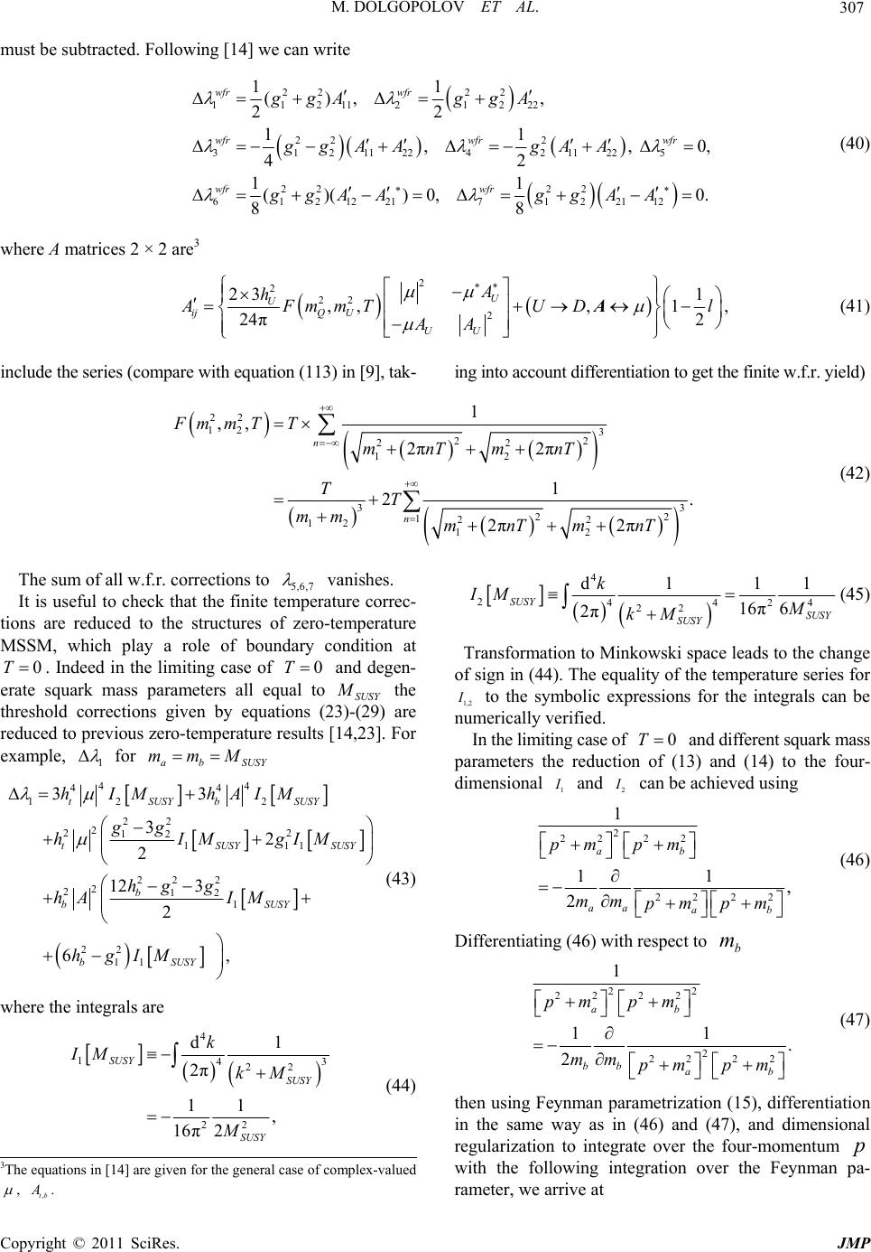 M. DOLGOPOLOV ET AL. Copyright © 2011 SciRes. JMP 307 must be subtracted. Following [14] we can write 22 22 1121121222 22 2 31211224211225 22 22 61 2122171 22112 11 (),, 22 11 ,,0, 42 11 ()( )0,0. 88 wfr wfr wfrwfr wfr wfr wfr ggA ggA ggAA gAA ggAA ggAA (40) where A matrices 2 × 2 are3 2 2 22 2 23 1 ,,,1 , 24 π2 U U ijQ U UU A h FmmTUDl AA A (41) include the series (compare with equation (113) in [9], tak- ing into account differentiation to get the finite w.f.r. yield) 22 12 3 22 22 12 33 22 122 12 12 1 ,, 2π2π 1 2. 2π2π n n Fmm TT mnTmnT TT mm mnTmnT (42) The sum of all w.f.r. corrections to 5,6,7 vanishes. It is useful to check that the finite temperature correc- tions are reduced to the structures of zero-temperature MSSM, which play a role of boundary condition at 0T. Indeed in the limiting case of 0T and degen- erate squark mass parameters all equal to SUSY M the threshold corrections given by equations (23)-(29) are reduced to previous zero-temperature results [14,23]. For example, 1 for abSUSY mmM 44 44 122 22 2 22 12 111 22 2 2 212 1 22 11 33 32 2 12 3 2 6, tSUSY bSUSY tSUSYSUSY b bSUSY bSUSY hIM hAIM gg hIMgIM hg g hA IM hgIM (43) where the integrals are 4 143 22 22 d1 2π 11 , 16 π2 SUSY SUSY SUSY k IM kM M (44) 4 24424 22 d1 11 16 π6 2π SUSY SUSY SUSY k IM M kM (45) Transformation to Minkowski space leads to the change of sign in (44). The equality of the temperature series for 1,2 to the symbolic expressions for the integrals can be numerically verified. In the limiting case of 0T and different squark mass parameters the reduction of (13) and (14) to the four- dimensional 1 and 2 can be achieved using 2 22 22 2222 1 11 , 2 ab aa ab pm pm mmpm pm (46) Differentiating (46) with respect to b m 22 22 22 2 22 22 1 11 . 2 ab bb ab pm pm mmpm pm (47) then using Feynman parametrization (15), differentiation in the same way as in (46) and (47), and dimensional regularization to integrate over the four-momentum with the following integration over the Feynman pa- rameter, we arrive at 3The equations in [14] are given for the general case of complex-valued , ,tb .  M. DOLGOPOLOV ET AL. Copyright © 2011 SciRes. JMP 308 4 142 22 22 22 2 222 d1 2π 12ln , 16 π ab a ab b ab p I pm pm m mm m mm (48) 4 2422 22 22 22 22 3 222 d1 2π ln . 8π ab a ab ab b ab p I pm pm m mm mmm mm (49) In the limit ab mm these formulas coincide with the expressions for degenerate squark masses (44) and (45). In calculations of the temperature dependent parame- ters iT of the effective MSSM potential at moderate temperatures truncated series with fifty terms (50 Ma- tsubara frequencies) were used. Relative contributions of the remaining terms are less than 10–2 percent at T = 50 GeV, decreasing with an increasing T. At small tem- peratures of the order of a few GeV an acceptable accu- racy is achieved with 1000 terms. The effective parame- ters iT are less than one, justifying the perturbative approach, as a rule, at the squark mass parameters around several hundred GeV. However, strong parametric de- pendence is observed here, for example, at the squark mass parameters 200, 500 and 800 GeV the criteria 1 iT is valid up to T 860 GeV, while taking degenerate squark masses at 600 GeV it turns out that at 600T GeV the perturbative regime cannot be used. 3. Thermal Evolution and the Critical Temperature In view of the effective two-doublet potential structure defined by (2) one could assume that the two-dimen- sional picture of a broken symmetry of 12 , eff Uvv with a local minima at 0T, 1,2 0v appears in the sum of the potential terms with 2 1 , 2 2 and 2 12 of dimen- sion 2 in the fields, which form a ‘saddle’ (a hyperboloid in the 12 ,vv space), and of the dimension 4 terms 1, ,7 which are increasing quartically, being unbounded from above. However, the situation is more involved because 2 1 , 2 2 , 2 12 and i respect a number of constraints. In this section we are going to describe roughly some possible scenarios of temperature evolu- tion in the effective two-doublet MSSM Higgs sector with threshold, logarithmic and wave-function renor- malization one-loop corrections. Two sets of the squark mass parameters in the following numerical calculations are used (A) 500 GeV, 200 GeV, 800 GeV, QU D mmm (B) 500 GeV, 800 GeV, 200 GeV. QU D mmm Masses of the third generation squarks are 22222 1,2 22222 1, 2 222 1 222 2 14, 2 14, 2 LR LR LR LR top ttttt b bbbbb mmmmmAm mmmmmAm where 2 2 2 2 22 22 222 2 22 22 222 2 12 cos 2sin, 23 2 cos 2sin, 3 11 cos 2sin, 23 1 cos 2sin 3 L R L R Qtop Zw t UtopZ w t Qb Zw b DbZ w b mmm m mmm m mmm m mmm m and 22 22 1, , 22 22 2, , cot2cot , tan2tan . tb tb tb tb AAA AA A With these parameters the third generation squark ei- genstates 1, 2 t m and 1,2 b m which masses are positively defined exist, as a rule, in an extensive regions of the (tan , , ) parameter space, see Figure 5. Set (A) favors the light stop, while the light sbottom is a feature of the parameter set (B). Fixed parameters for the plots in Figure 5 are tan 5 , ,1 tb A TeV, 1.5 TeV, 180 H m GeV. Squark masses vary in the range from 200 GeV to 800 GeV at the values of ,tb and up to the order of 1 TeV. Large difference of the stop masses is necessary to respect constraints following from the LEP2 experimental limit 11 5 h m GeV. The values of tan above 5 and large soft supersymmetry break- ing parameters ,tb and of the order of Q m also lead to an acceptable Higgs boson mass h m (but weaken the strength of the electroweak phase transition if taken too large). At the same time substantial threshold correc- tions appear in the MSSM scenarios with large ,tb and , like the BGX scenario [24] and the CPX scenario [25], or the regions of MSSM parameter space close to BGX and CPX. In the following the equilibrium states of effective po- tential (2) as a function of the two variables of state 1 v and 2 v and six temperature-dependent control parame- ters 17 ,,TT are going to be analysed. Local pro- 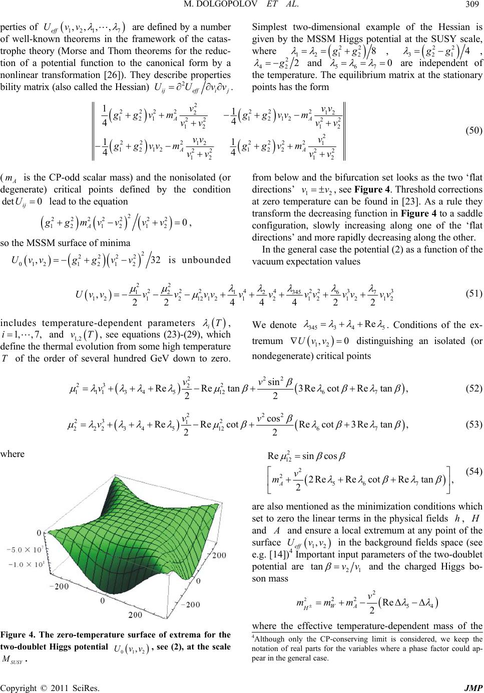 M. DOLGOPOLOV ET AL. Copyright © 2011 SciRes. JMP 309 perties of 12 17 ,,, , eff Uvv are defined by a number of well-known theorems in the framework of the catas- trophe theory (Morse and Thom theorems for the reduc- tion of a potential function to the canonical form by a nonlinear transformation [26]). They describe properties bility matrix (also called the Hessian) 2 ijeffij UUvv . Simplest two-dimensional example of the Hessian is given by the MSSM Higgs potential at the SUSY scale, where 22 1212 8gg , 22 321 4gg , 2 42 2g and 567 0 are independent of the temperature. The equilibrium matrix at the stationary points has the form 2 2222222 212 1211212 22 22 12 12 2 2222222 12 1 1212 122 22 22 12 12 11 4 4 11 44 AA AA vvv ggvm ggvvm vv vv vv v ggvvmggvm vv vv (50) (A m is the CP-odd scalar mass) and the nonisolated (or degenerate) critical points defined by the condition det 0 ij U lead to the equation 2 22222 22 1212 12 0 A ggmvv vv, so the MSSM surface of minima 2 2222 0121212 ,32Uvvggv v is unbounded from below and the bifurcation set looks as the two ‘flat directions’ 12 vv , see Figure 4. Threshold corrections at zero temperature can be found in [23]. As a rule they transform the decreasing function in Figure 4 to a saddle configuration, slowly increasing along one of the ‘flat directions’ and more rapidly decreasing along the other. In the general case the potential (2) as a function of the vacuum expectation values 22 222442233 3456 7 12 12 12121212121 21 212 ,2244422 Uvvvvvv vvvvvvvv (51) includes temperature-dependent parameters iT , 1,, 7,i and 1, 2 vT , see equations (23)-(29), which define the thermal evolution from some high temperature T of the order of several hundred GeV down to zero. We denote 3453 45 Re . Conditions of the ex- tremum 12 ,0Uvv distinguishing an isolated (or nondegenerate) critical points 222 23 2 2 111 3451267 sin ReRetan3Re cotRe tan, 22 vv v (52) 222 23 2 1 222 3451267 cos ReRecotRe cot3Retan, 22 vv v (53) where Figure 4. The zero-temperature surface of extrema for the two-doublet Higgs potential 012 ,Uvv, see (2), at the scale SUSY . 2 12 2 2 56 7 Resincos 2ReRecotRe tan, 2 A v m (54) are also mentioned as the minimization conditions which set to zero the linear terms in the physical fields h, and and ensure a local extremum at any point of the surface 12 , eff Uvv in the background fields space (see e.g. [14])4 Important input parameters of the two-doublet potential are 21 tan vv and the charged Higgs bo- son mass 2 2 22 54 Re 2 WA H v mmm where the effective temperature-dependent mass of the 4Although only the CP-conserving limit is considered, we keep the notation of real parts for the variables where a phase factor could ap- ear in the general case. 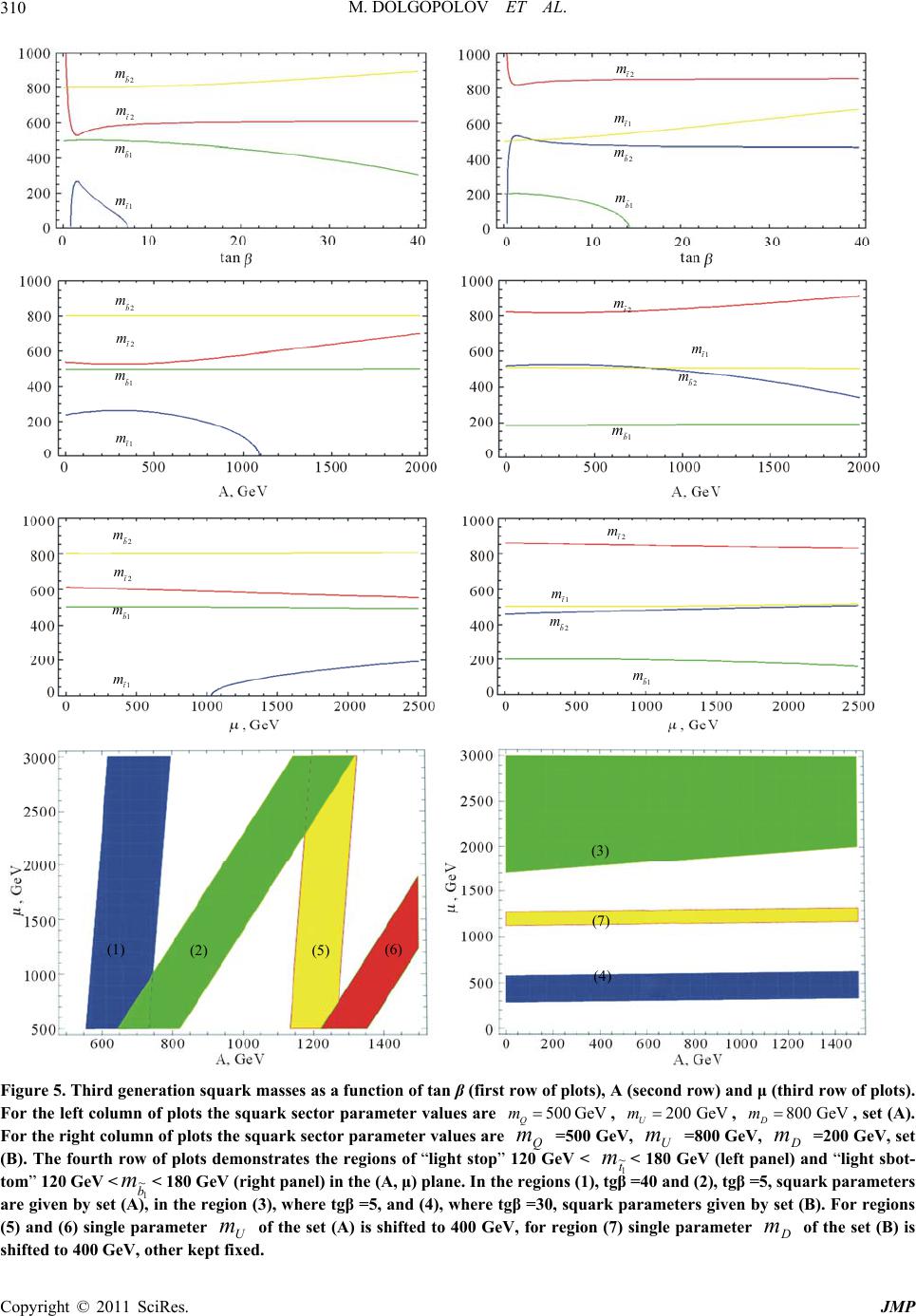 M. DOLGOPOLOV ET AL. Copyright © 2011 SciRes. JMP 310 2t m 2b m 1b m 1t m 2t m 2b m 1b m 1t m 2t m 2b m 1b m 1t m 2t m 2b m 1b m 1t m 2t m 2b m 1b m 1t m 2t m 2b m 1b m 1t m (1) (2) (5) (6) (3) (7) (4) Figure 5. Third generation squark masses as a function of tan β (first row of plots), A (second row) and μ (third row of plots). For the left column of plots the squark sector parameter values are 500 GeV Q m , 200 GeV U m , 800 GeV D m, set (A). For the right column of plots the squark sector parameter values are Q m =500 GeV, U m =800 GeV, D m =200 GeV, set (B). The fourth row of plots demonstrates the regions of “light stop” 120 GeV < 1 ~ t m< 180 GeV (left panel) and “light sbot- tom” 120 GeV < 1 ~ b m< 180 GeV (right panel) in the (A, μ) plane. In the regions (1), tgβ =40 and (2), tgβ =5, squark parameters are given by set (A), in the region (3), where tgβ =5, and (4), where tgβ =30, squark parameters given by set (B). For regions (5) and (6) single parameter U m of the set (A) is shifted to 400 GeV, for region (7) single parameter D m of the set (B) is shifted to 400 GeV, other kept fixed. 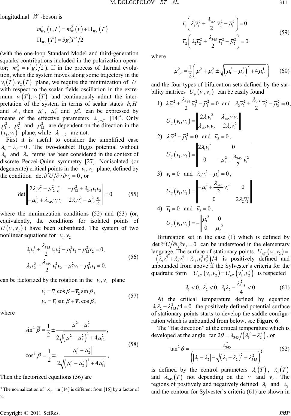 M. DOLGOPOLOV ET AL. Copyright © 2011 SciRes. JMP 311 longitudinal W-boson is 22 22 2 , 52 LL L WWW W mvT mvT TgT (with the one-loop Standard Model and third-generation squarks contributions included in the polarization opera- tor; 222 22 W mvg). If in the process of thermal evolu- tion, when the system moves along some trajectory in the 12 ,vT vT plane, we require the minimization of U with respect to the scalar fields oscillation in the extre- mum 12 ,vT vT and continuously admit the inter- pretation of the system in terms of scalar states ,hH and , then 2 1 , 2 2 and 4 12 can be expressed by means of the effective parameters 1, ,7 [14]4. Only 2 1 , 2 2 and 2 12 are dependent on the direction in the 12 ,vv plane, while 1, ,7 are not. First it is useful to consider the simplified case 67 0 . The two-doublet Higgs potential without 6 and 7 terms has been considered in the context of discrete Peccei-Quinn symmetry [27]. Nonisolated (or degenerate) critical points in the 12 ,vv plane, defined by the condition 2 det 0 ij Uvv, or 2 1 1 2 222 1 1121234512 222 12345 1 22212 2 det 0 2 v v v v vvv vv v (55) where the minimization conditions (52) and (53) (or, equivalently, the conditions for isolated points of 12 ,Uvv ) have been substituted. The system of two nonlinear equations for 12 ,vv 3222 345 11121112 2 3222 345 221 22 2121 0, 2 0. 2 vvvvv vvvvv (56) can be factorized by the rotation in the 12 ,vv plane 11 2 21 2 cossin, sincos , vv v vv v (57) where 22 12 2 2 22 2 12 12 22 12 2 2 22 2 12 12 1 sin , 224 1 cos , 224 (58) Then the factorized equations (56) are 222 345 1112 1 222 345 2221 2 0 2 0 2 vv v vv v (59) where 2 222224 1,2121 212 14 2 (60) and the four types of bifurcation sets defined by the sta- bility matrices 12 , ij Uvv can be easily found 1) 222 345 11210 2 vv and 222 345 2212 0 2 vv , 2 1 134512 12 2 345 1 222 2 ,2 ij vvv Uvv vv v 2) 22 111 0v and 20v, 2 11 12 22 345 21 20 ,02 ij v Uvv v 3) 10v and 22 222 0v , 22 345 12 12 2 22 0 ,2 02 ij v Uvv v 4) 10v and 20v , 2 1 12 2 2 0 ,0 ij Uvv Bifurcation set in the case (1) which is defined by 2 det 0 ij Uvv can be understood in the elementary language. The surface of stationary points 12 , eff Uvv 44 22 1 122345124vv vv is positively defined and unbounded from above if the Sylvester’s criteria for the quadratic form 22 121 2 ,, eff eff Uvv Uvv is respected 2 345 1212 0, 0,0 4 (61) At the critical temperature defined by equation 2 1 2345 40 the positively defined potential surface of stationary points starts to develop the saddle configu- ration which is unbounded from below, see Figure 6. The “flat direction” at the critical temperature which is developed at the angle 22 345 12 tan2 , or 2 2345 2 22 1 21 2345 tan (62) is defined by the control parameters 1T , 2T and 345 T not depending on the 1 v and 2 v. The regions of positively and negatively defined 1 and 2 and the contour for Sylvester’s criteria (61) are shown in 4 The normalization of 1,2 in [14] is different from [15] by a factor o 2. 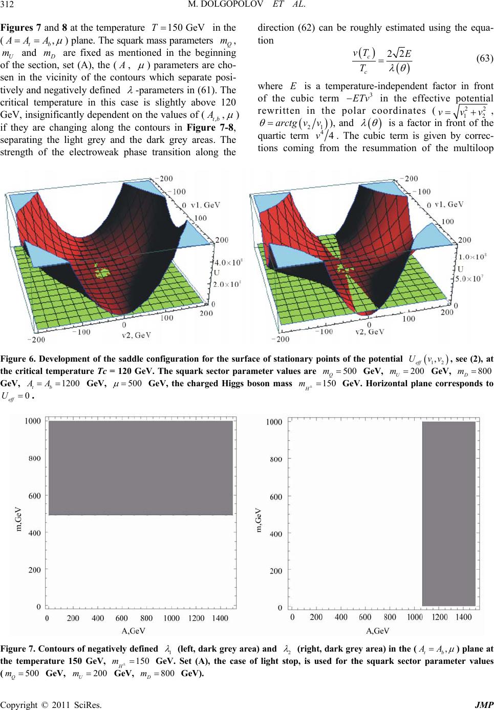 M. DOLGOPOLOV ET AL. Copyright © 2011 SciRes. JMP 312 Figures 7 and 8 at the temperature 150 GeVT in the (, tb AA A ) plane. The squark mass parameters Q m, U m and m are fixed as mentioned in the beginning of the section, set (A), the ( , ) parameters are cho- sen in the vicinity of the contours which separate posi- tively and negatively defined -parameters in (61). The critical temperature in this case is slightly above 120 GeV, insignificantly dependent on the values of (,tb , ) if they are changing along the contours in Figure 7-8, separating the light grey and the dark grey areas. The strength of the electroweak phase transition along the direction (62) can be roughly estimated using the equa- tion 22 c c vT E T (63) where E is a temperature-independent factor in front of the cubic term 3 ETv in the effective potential rewritten in the polar coordinates (22 12 vvv , 21 arctg vv ), and is a factor in front of the quartic term 44v. The cubic term is given by correc- tions coming from the resummation of the multiloop Figure 6. Development of the saddle configuration for the surface of stationary points of the potential 12 , eff Uvv , see (2), at the critical temperature Tc = 120 GeV. The squark sector parameter values are 500 Q m GeV, 200 U m GeV, 800 D m GeV, 1200 tb AA GeV, 500 GeV, the charged Higgs boson mass 150 H m GeV. Horizontal plane corresponds to 0 eff U. Figure 7. Contours of negatively defined 1 (left, dark grey area) and 2 (right, dark grey area) in the (, tb AA ) plane at the temperature 150 GeV, 150 H m GeV. Set (A), the case of light stop, is used for the squark sector parameter values (500 Q m GeV, 200 U m GeV, 800 D m GeV). 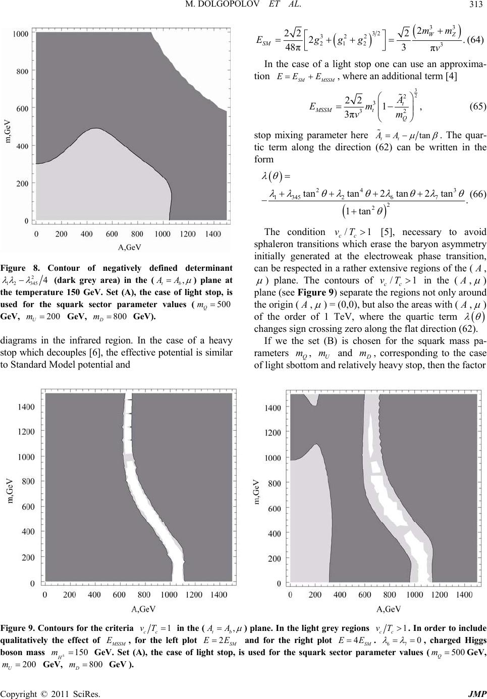 M. DOLGOPOLOV ET AL. Copyright © 2011 SciRes. JMP 313 Figure 8. Contour of negatively defined determinant 2 12 3454 (dark grey area) in the (, tb AA ) plane at the temperature 150 GeV. Set (A), the case of light stop, is used for the squark sector parameter values (500 Q m GeV, 200 U m GeV, 800 D m GeV). diagrams in the infrared region. In the case of a heavy stop which decouples [6], the effective potential is similar to Standard Model potential and 33 32 322 212 3 2 22 2 2. 48π3π WZ SM mm Eggg v (64) In the case of a light stop one can use an approxima- tion SM MSSM EE E , where an additional term [4] 3 2 2 3 32 22 1, 3π t MSSM t Q A Em vm (65) stop mixing parameter here tan tt AA . The quar- tic term along the direction (62) can be written in the form 24 3 1 345267 2 2 tantan2 tan2 tan. 1tan (66) The condition /1 cc vT [5], necessary to avoid sphaleron transitions which erase the baryon asymmetry initially generated at the electroweak phase transition, can be respected in a rather extensive regions of the ( , ) plane. The contours of /1 cc vT in the ( , ) plane (see Figure 9) separate the regions not only around the origin ( , ) = (0,0), but also the areas with ( , ) of the order of 1 TeV, where the quartic term changes sign crossing zero along the flat direction (62). If we the set (B) is chosen for the squark mass pa- rameters Q m, U m and m, corresponding to the case of light sbottom and relatively heavy stop, then the factor Figure 9. Contours for the criteria 1 cc vT in the (, tb AA ) plane. In the light grey regions 1 cc vT. In order to include qualitatively the effect of SSM E, for the left plot 2SM EE and for the right plot 4SM EE . 67 0 , charged Higgs boson mass 150 H m GeV. Set (A), the case of light stop, is used for the squark sector parameter values (500 Q m GeV, 200 U m GeV, 800 D m GeV ). 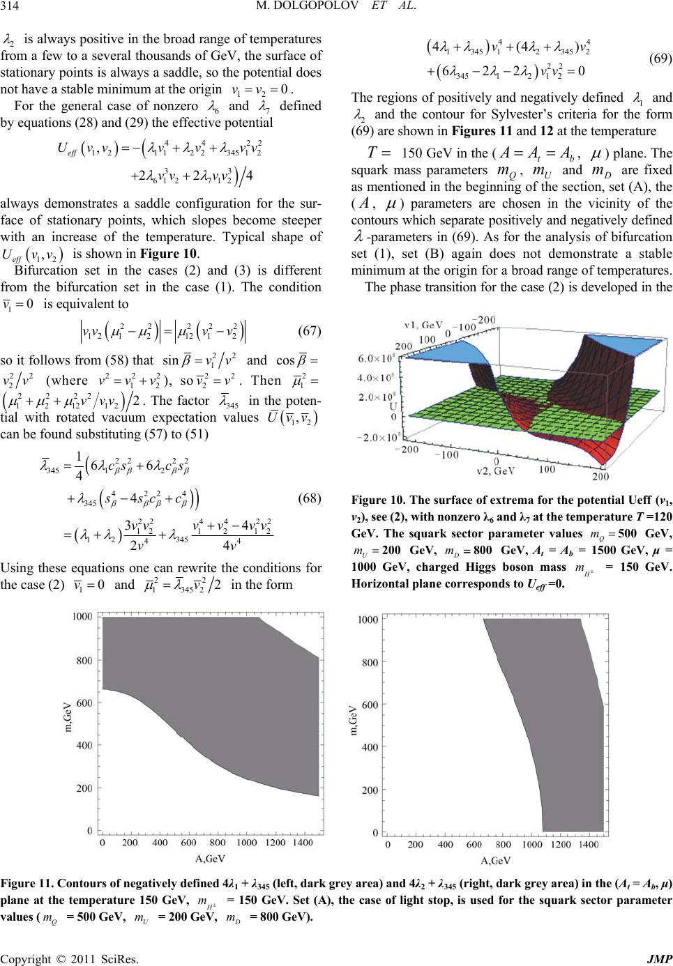 M. DOLGOPOLOV ET AL. Copyright © 2011 SciRes. JMP 314 2 is always positive in the broad range of temperatures from a few to a several thousands of GeV, the surface of stationary points is always a saddle, so the potential does not have a stable minimum at the origin 12 0vv. For the general case of nonzero 6 and 7 defined by equations (28) and (29) the effective potential 44 22 121 12234512 33 61 2712 , 224 eff Uvvv vvv vv vv always demonstrates a saddle configuration for the sur- face of stationary points, which slopes become steeper with an increase of the temperature. Typical shape of 12 , eff Uvv is shown in Figure 10. Bifurcation set in the cases (2) and (3) is different from the bifurcation set in the case (1). The condition 10v is equivalent to 22 222 12121212 vvv v (67) so it follows from (58) that 22 1 sin vv and cos 22 2 vv (where 222 12 vvv), so22 2 vv. Then 2 1 2222 121212 2vvv . The factor 345 in the poten- tial with rotated vacuum expectation values 12 ,Uvv can be found substituting (57) to (51) 22 22 345 12 4224 345 224 422 121 212 1 2345 44 166 4 4 34 24 cs cs sscc vvv vvv vv (68) Using these equations one can rewrite the conditions for the case (2) 10v and 22 1345 22v in the form 44 134512345 2 22 3451212 4(4) 6220 vv vv (69) The regions of positively and negatively defined 1 and 2 and the contour for Sylvester’s criteria for the form (69) are shown in Figures 11 and 12 at the temperature 150 GeV in the (bt AAA , ) plane. The squark mass parameters Q m, U m and D m are fixed as mentioned in the beginning of the section, set (A), the (A, ) parameters are chosen in the vicinity of the contours which separate positively and negatively defined -parameters in (69). As for the analysis of bifurcation set (1), set (B) again does not demonstrate a stable minimum at the origin for a broad range of temperatures. The phase transition for the case (2) is developed in the Figure 10. The surface of extrema for the potential Ueff (v1, v2), see (2), with nonzero λ6 and λ7 at the temperature T =120 GeV. The squark sector parameter values Q m 500 GeV, U m 200 GeV, D m800 GeV, At = Ab = 1500 GeV, μ = 1000 GeV, charged Higgs boson mass m = 150 GeV. Horizontal plane corresponds to Ueff =0. Figure 11. Contours of negatively defined 4λ1 + λ345 (left, dark grey area) and 4λ2 + λ345 (right, dark grey area) in the (At = Ab, μ) plane at the temperature 150 GeV, m = 150 GeV. Set (A), the case of light stop, is used for the squark sector parameter values (Q m = 500 GeV, U m = 200 GeV, m = 800 GeV).  M. DOLGOPOLOV ET AL. Copyright © 2011 SciRes. JMP 315 Figure 12. Contour of negatively defined determinant (4λ1 + λ345)(4λ2 + λ345) − (3λ345 − λ1 − λ2)2 (dark grey area) in the (At = Ab, μ) plane at the temperature 150 GeV. Set (A), the case of light stop, is used for the squark sector parameter values (mQ =500 GeV, mU =200 GeV, mD = 800 GeV). direction of the 12 ,vv plane 345 1 2 22 1 3452 345 33 tan 244 (70) Bifurcation set in the case (4) 10v and 20v de- fined by the equation 22 12 0 can also be understood on the elementary level as a result of the diagonalization of the effective potential 22 22222 12 121212 22 eff Uvvvv by the rotation (57), giving the form 2222 11 22 eff Uvv . This case is inter- esting not only in the case of an effective field theory under consideration but also in a more general physical framework. So far it has been assumed that we are in the framework of an effective field theory at the top m en- ergy scale, when the contributions from squarks decouple or a contribution of the potential terms with squarks (see the Appendix) is practically constant. However, if it is not the case and the Higgs bosons-squarks quartic term is positive definite with the global minimum at the origin 12 0vv, the phase transition may occur due to the development of a saddle configuration by the 2 1 , 2 2 and 2 12 terms. Such situation may take place when the vacuum ex- pectation values of charged and colored superpartners participate in the full MSSM scalar potential, possibly giving charge and color breaking minima [28]. For illus- trative purposes it is convenient to use the polar coordi- nates 12 cos ,sinvT vTTvT vTT for the vacuum expectation values. The mass term of the two-doublet potential has the form 22 22 222 12 12 ,cossinsin 2 22 mass vv Uv (71) By definition at the critical temperature the gradient of , mass Uv is zero along some direction in the (1 v,2 v) plane, then 0 mass Uv and 10 mass vU ; it follows from these two equations 2 12 22 12 2 22 42 24 1 2121212 2 tan 2, 40 (72) The first of these equations is equivalent to (58). The phase transition is characterized by the critical angle T which defines the flat direction4 for the mass term at the temperature c T in the background fields plane 12 ,vv , and at the real-valued 1 , 2 and 12 the critical temperature is defined by the equation 224 12 12 (73) which is equivalent to 2 10 or 2 20 . For a fixed set of the squark sector parameters5 the thermodynamical evolution of the effective potential is described by a 0 eff nU trajectory in the three-dimensional (v, T, tan ) space, which is defined by the intersection of the two surfaces, corresponding to the equation (72) for the critical angle (“ -surface”), and the equation (73) for the 1 , 2 and 12 (“ -surface”). The cross sections of -surface (calculated without any approximations numerically) by the plane at fixed 0T, giving the (v, tan ) contour, and the cross section at tan giving the (v,T) contour is shown in Figure 13. The presence of nonzero effective parameters 6 and 7 is essential to get the critical temperature of the order of 100 GeV. Useful analytical approximation can be obtained using the minimization conditions (52)-(53), then the critical angle T defined by (72) can be expressed as7 5Flat directions may exist also in the quartic term separately taken, see e.g. [29]. 6Mathematica package [30] with encoded representations of iT by means of series with n = 50 was used to scan the MSSM parame- ter space. At low temperatures the convergence of Matsubara series becomes worse, so the number of terms up to n = 1000 is needed to reach an acceptable accuracy. 7In different context analogous relation between tan and tan can be found in [6], where the mass term of the form 2,vf T with 2 ,fTaTb was analyzed for a special case of degener- ate squark masses, 0 A and within the high-temperature expan- sion. Our quartic potential is very different from the tree-level 22 42 12 8cos 2 T ggv plus a logarithmic term [6], so the expression 3/1 T E of Bochkarev-Shaposhnikov criteria 1 cc vT Tfor the absence of sphaleron in the broken phase gives different results with nonzero threshold corrections. 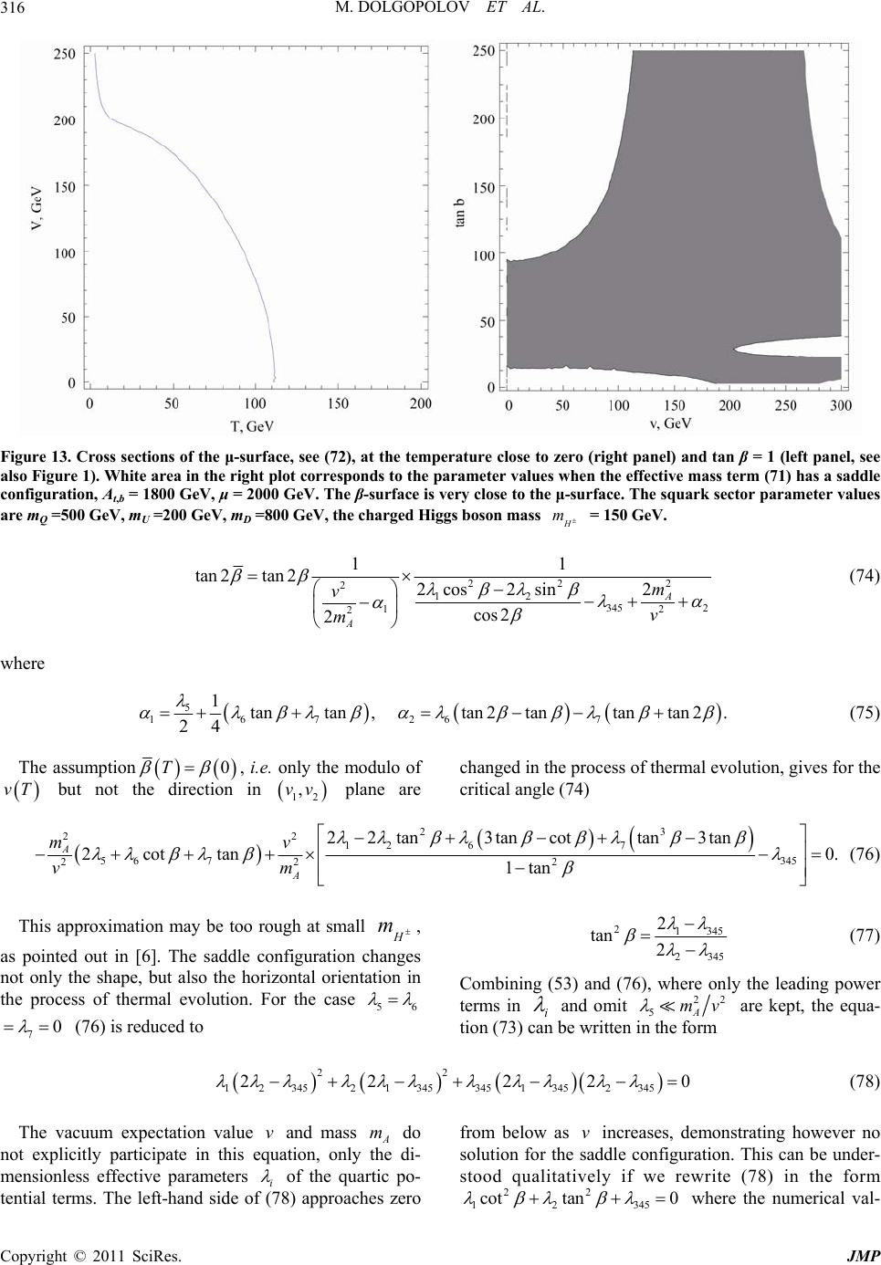 M. DOLGOPOLOV ET AL. Copyright © 2011 SciRes. JMP 316 Figure 13. Cross sections of the μ-surface, see (72), at the temperature close to zero (right panel) and tan β = 1 (left panel, see also Figure 1). White area in the right plot corresponds to the parameter values when the effective mass term (71) has a saddle configuration, At,b = 1800 GeV, μ = 2000 GeV. The β-surface is very close to the μ-surface. The squark sector parameter values are mQ =500 GeV, mU =200 GeV, mD =800 GeV, the charged Higgs boson mass m = 150 GeV. 22 2 2 12 345 2 2 1 2 11 tan 2tan22cos2sin2 cos 2 2 A A m v v m (74) where 5 167 267 1tantan, tan2tantantan2. 24 (75) The assumption 0T , i.e. only the modulo of vT but not the direction in 12 ,vv plane are changed in the process of thermal evolution, gives for the critical angle (74) 23 22 12 67 56 7345 22 2 22 tan3tancottan3tan 2cottan 0. 1tan A A mv vm (76) This approximation may be too rough at small H m, as pointed out in [6]. The saddle configuration changes not only the shape, but also the horizontal orientation in the process of thermal evolution. For the case 56 70 (76) is reduced to 21345 2 345 2 tan 2 (77) Combining (53) and (76), where only the leading power terms in i and omit 22 5A mv are kept, the equa- tion (73) can be written in the form 22 1234521 3453451 3452345 22 220 (78) The vacuum expectation value v and mass A m do not explicitly participate in this equation, only the di- mensionless effective parameters i of the quartic po- tential terms. The left-hand side of (78) approaches zero from below as v increases, demonstrating however no solution for the saddle configuration. This can be under- stood qualitatively if we rewrite (78) in the form 22 1 2345 cot tan0 where the numerical val- 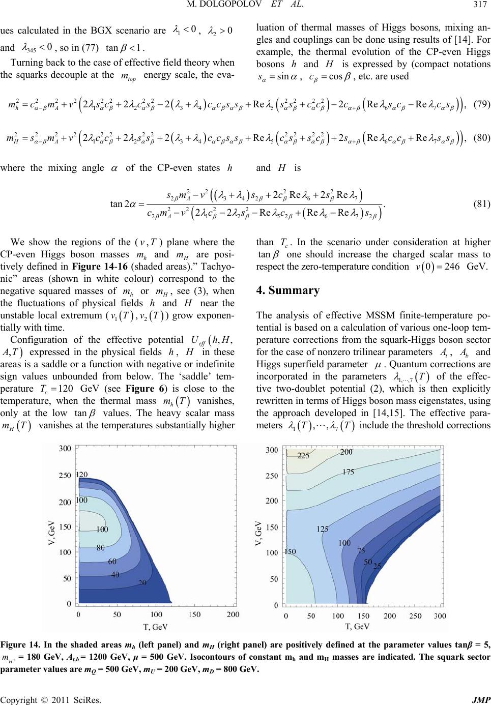 M. DOLGOPOLOV ET AL. Copyright © 2011 SciRes. JMP 317 ues calculated in the BGX scenario are 10 , 20 and 3450 , so in (77) tan 1 . Turning back to the case of effective field theory when the squarks decouple at the top m energy scale, the eva- luation of thermal masses of Higgs bosons, mixing an- gles and couplings can be done using results of [14]. For example, the thermal evolution of the CP-even Higgs bosons h and is expressed by (compact notations sins , cosc , etc. are used 2222222222 22 12 34567 222Re2Re Re , hA mcmvsccsccsssscccsccs (79) 222 2222222 22 12 34567 222Re2 ReRe, HA msmvccssccsscsscsccss (80) where the mixing angle of the CP-even states h and is 2222 234267 22 22 21252672 2Re2Re tan 2. 22ReRe Re A A sm vscs cm vcscs (81) We show the regions of the (v,T) plane where the CP-even Higgs boson masses h m and m are posi- tively defined in Figure 14-16 (shaded areas).” Tachyo- nic” areas (shown in white colour) correspond to the negative squared masses of h m or m, see (3), when the fluctuations of physical fields h and near the unstable local extremum ( 1 vT, 2 vT ) grow exponen- tially with time. Configuration of the effective potential ,, eff UhH , T expressed in the physical fields h, in these areas is a saddle or a function with negative or indefinite sign values unbounded from below. The ‘saddle’ tem- perature 120 c T GeV (see Figure 6) is close to the temperature, when the thermal mass h mT vanishes, only at the low tan values. The heavy scalar mass H mT vanishes at the temperatures substantially higher than c T. In the scenario under consideration at higher tan one should increase the charged scalar mass to respect the zero-temperature condition 0 246v GeV. 4. Summary The analysis of effective MSSM finite-temperature po- tential is based on a calculation of various one-loop tem- perature corrections from the squark-Higgs boson sector for the case of nonzero trilinear parameters t , b and Higgs superfield parameter . Quantum corrections are incorporated in the parameters 1, ,7T of the effec- tive two-doublet potential (2), which is then explicitly rewritten in terms of Higgs boson mass eigenstates, using the approach developed in [14,15]. The effective para- meters 17 ,,TT include the threshold corrections Figure 14. In the shaded areas mh (left panel) and mH (right panel) are positively defined at the parameter values tanβ = 5, m= 180 GeV, At,b = 1200 GeV, μ = 500 GeV. Isocontours of constant mh and mH masses are indicated. The squark sector parameter values are mQ = 500 GeV, mU = 200 GeV, mD = 800 GeV. 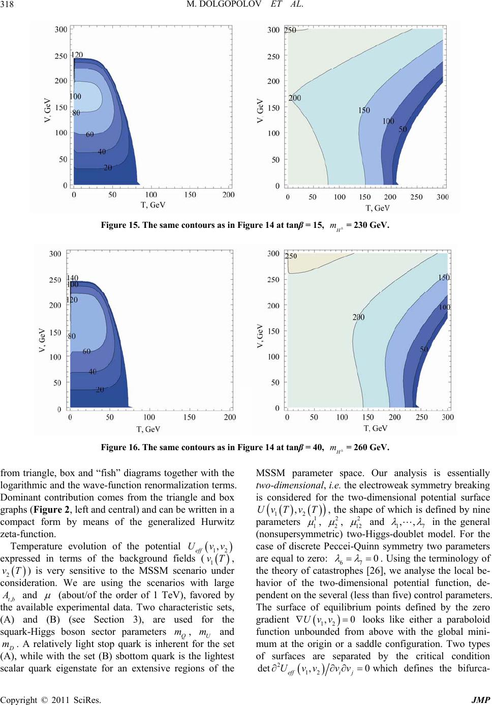 M. DOLGOPOLOV ET AL. Copyright © 2011 SciRes. JMP 318 Figure 15. The same contours as in Figure 14 at tanβ = 15, m = 230 GeV. Figure 16. The same contours as in Figure 14 at tanβ = 40, m = 260 GeV. from triangle, box and “fish” diagrams together with the logarithmic and the wave-function renormalization terms. Dominant contribution comes from the triangle and box graphs (Figure 2, left and central) and can be written in a compact form by means of the generalized Hurwitz zeta-function. Temperature evolution of the potential 12 , eff Uvv expressed in terms of the background fields ( 1 vT, 2 vT) is very sensitive to the MSSM scenario under consideration. We are using the scenarios with large ,tb and (about/of the order of 1 TeV), favored by the available experimental data. Two characteristic sets, (A) and (B) (see Section 3), are used for the squark-Higgs boson sector parameters Q m, U m and m. A relatively light stop quark is inherent for the set (A), while with the set (B) sbottom quark is the lightest scalar quark eigenstate for an extensive regions of the MSSM parameter space. Our analysis is essentially two-dimensional, i.e. the electroweak symmetry breaking is considered for the two-dimensional potential surface 12 ,UvTvT, the shape of which is defined by nine parameters 1 1 , 2 2 , 2 12 and 17 ,, in the general (nonsupersymmetric) two-Higgs-doublet model. For the case of discrete Peccei-Quinn symmetry two parameters are equal to zero: 67 0 . Using the terminology of the theory of catastrophes [26], we analyse the local be- havior of the two-dimensional potential function, de- pendent on the several (less than five) control parameters. The surface of equilibrium points defined by the zero gradient 12 ,0Uvv looks like either a paraboloid function unbounded from above with the global mini- mum at the origin or a saddle configuration. Two types of surfaces are separated by the critical condition 2 12 det ,0 effi j Uvvvv which defines the bifurca- 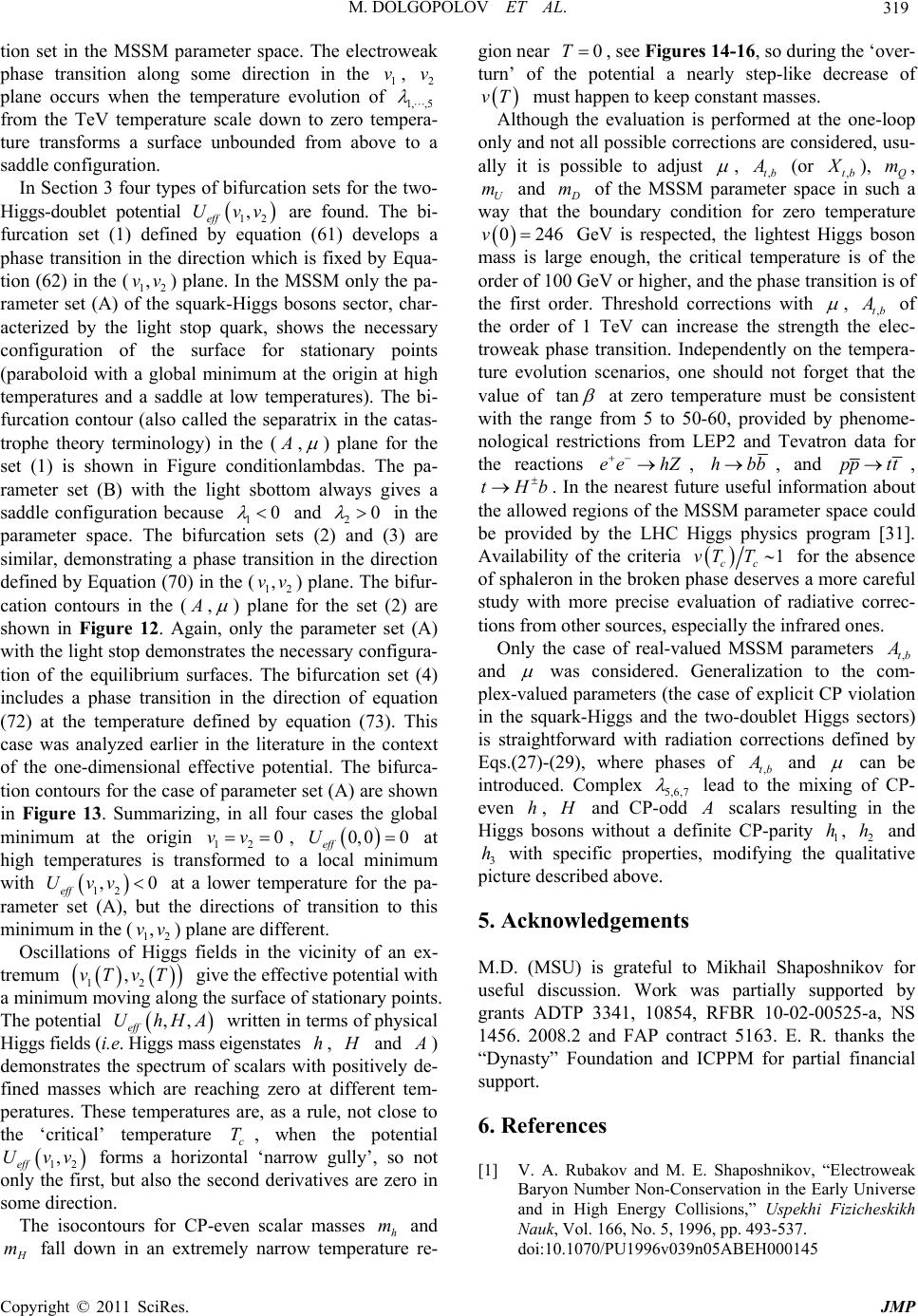 M. DOLGOPOLOV ET AL. Copyright © 2011 SciRes. JMP 319 tion set in the MSSM parameter space. The electroweak phase transition along some direction in the 1 v, 2 v plane occurs when the temperature evolution of 1, ,5 from the TeV temperature scale down to zero tempera- ture transforms a surface unbounded from above to a saddle configuration. In Section 3 four types of bifurcation sets for the two- Higgs-doublet potential 12 , eff Uvv are found. The bi- furcation set (1) defined by equation (61) develops a phase transition in the direction which is fixed by Equa- tion (62) in the (12 ,vv) plane. In the MSSM only the pa- rameter set (A) of the squark-Higgs bosons sector, char- acterized by the light stop quark, shows the necessary configuration of the surface for stationary points (paraboloid with a global minimum at the origin at high temperatures and a saddle at low temperatures). The bi- furcation contour (also called the separatrix in the catas- trophe theory terminology) in the ( , ) plane for the set (1) is shown in Figure conditionlambdas. The pa- rameter set (B) with the light sbottom always gives a saddle configuration because 10 and 20 in the parameter space. The bifurcation sets (2) and (3) are similar, demonstrating a phase transition in the direction defined by Equation (70) in the (12 ,vv) plane. The bifur- cation contours in the ( , ) plane for the set (2) are shown in Figure 12. Again, only the parameter set (A) with the light stop demonstrates the necessary configura- tion of the equilibrium surfaces. The bifurcation set (4) includes a phase transition in the direction of equation (72) at the temperature defined by equation (73). This case was analyzed earlier in the literature in the context of the one-dimensional effective potential. The bifurca- tion contours for the case of parameter set (A) are shown in Figure 13. Summarizing, in all four cases the global minimum at the origin 12 0vv , 0, 00 eff U at high temperatures is transformed to a local minimum with 12 ,0 eff Uvv at a lower temperature for the pa- rameter set (A), but the directions of transition to this minimum in the (12 ,vv) plane are different. Oscillations of Higgs fields in the vicinity of an ex- tremum 12 ,vTv T give the effective potential with a minimum moving along the surface of stationary points. The potential ,, eff UhHA written in terms of physical Higgs fields (i.e. Higgs mass eigenstates h, and ) demonstrates the spectrum of scalars with positively de- fined masses which are reaching zero at different tem- peratures. These temperatures are, as a rule, not close to the ‘critical’ temperature c T, when the potential 12 , eff Uvv forms a horizontal ‘narrow gully’, so not only the first, but also the second derivatives are zero in some direction. The isocontours for CP-even scalar masses h m and m fall down in an extremely narrow temperature re- gion near 0T , see Figures 14-16, so during the ‘over- turn’ of the potential a nearly step-like decrease of vT must happen to keep constant masses. Although the evaluation is performed at the one-loop only and not all possible corrections are considered, usu- ally it is possible to adjust , ,tb (or ,tb ), Q m, U m and m of the MSSM parameter space in such a way that the boundary condition for zero temperature 0 246v GeV is respected, the lightest Higgs boson mass is large enough, the critical temperature is of the order of 100 GeV or higher, and the phase transition is of the first order. Threshold corrections with , ,tb of the order of 1 TeV can increase the strength the elec- troweak phase transition. Independently on the tempera- ture evolution scenarios, one should not forget that the value of tan at zero temperature must be consistent with the range from 5 to 50-60, provided by phenome- nological restrictions from LEP2 and Tevatron data for the reactions ee hZ , hbb, and pp tt, tHb . In the nearest future useful information about the allowed regions of the MSSM parameter space could be provided by the LHC Higgs physics program [31]. Availability of the criteria 1 cc vT T for the absence of sphaleron in the broken phase deserves a more careful study with more precise evaluation of radiative correc- tions from other sources, especially the infrared ones. Only the case of real-valued MSSM parameters ,tb and was considered. Generalization to the com- plex-valued parameters (the case of explicit CP violation in the squark-Higgs and the two-doublet Higgs sectors) is straightforward with radiation corrections defined by Eqs.(27)-(29), where phases of ,tb and can be introduced. Complex 5,6,7 lead to the mixing of CP- even h, and CP-odd scalars resulting in the Higgs bosons without a definite CP-parity 1 h, 2 h and 3 h with specific properties, modifying the qualitative picture described above. 5. Acknowledgements M.D. (MSU) is grateful to Mikhail Shaposhnikov for useful discussion. Work was partially supported by grants ADTP 3341, 10854, RFBR 10-02-00525-a, NS 1456. 2008.2 and FAP contract 5163. E. R. thanks the “Dynasty” Foundation and ICPPM for partial financial support. 6. References [1] V. A. Rubakov and M. E. Shaposhnikov, “Electroweak Baryon Number Non-Conservation in the Early Universe and in High Energy Collisions,” Uspekhi Fizicheskikh Nauk, Vol. 166, No. 5, 1996, pp. 493-537. doi:10.1070/PU1996v039n05ABEH000145 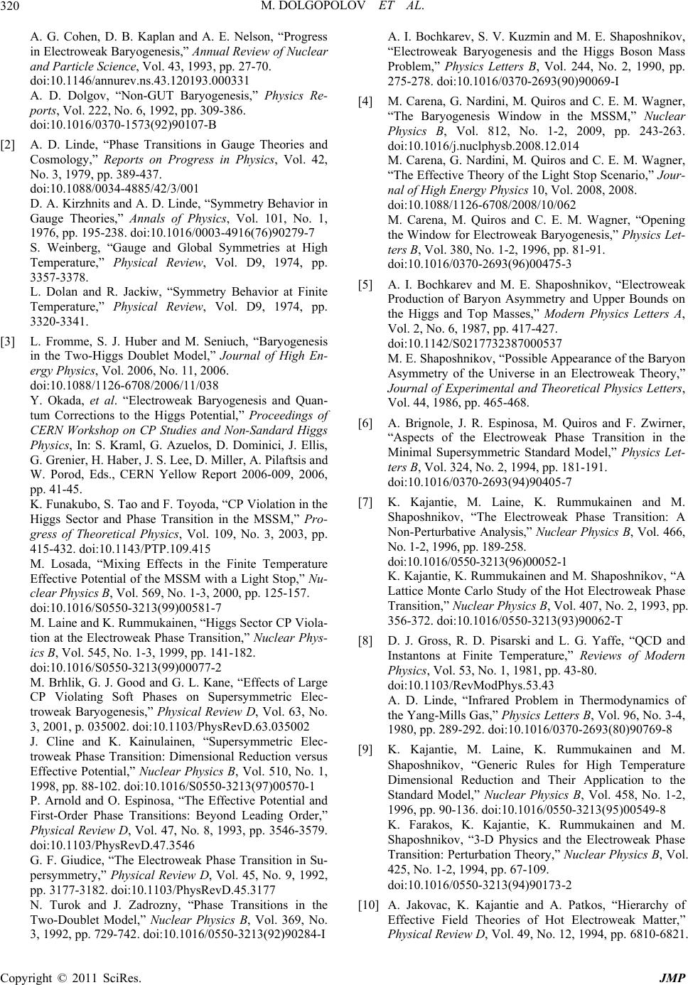 M. DOLGOPOLOV ET AL. Copyright © 2011 SciRes. JMP 320 A. G. Cohen, D. B. Kaplan and A. E. Nelson, “Progress in Electroweak Baryogenesis,” Annual Review of Nuclear and Particle Science, Vol. 43, 1993, pp. 27-70. doi:10.1146/annurev.ns.43.120193.000331 A. D. Dolgov, “Non-GUT Baryogenesis,” Physics Re- ports, Vol. 222, No. 6, 1992, pp. 309-386. doi:10.1016/0370-1573(92)90107-B [2] A. D. Linde, “Phase Transitions in Gauge Theories and Cosmology,” Reports on Progress in Physics, Vol. 42, No. 3, 1979, pp. 389-437. doi:10.1088/0034-4885/42/3/001 D. A. Kirzhnits and A. D. Linde, “Symmetry Behavior in Gauge Theories,” Annals of Physics, Vol. 101, No. 1, 1976, pp. 195-238. doi:10.1016/0003-4916(76)90279-7 S. Weinberg, “Gauge and Global Symmetries at High Temperature,” Physical Review, Vol. D9, 1974, pp. 3357-3378. L. Dolan and R. Jackiw, “Symmetry Behavior at Finite Temperature,” Physical Review, Vol. D9, 1974, pp. 3320-3341. [3] L. Fromme, S. J. Huber and M. Seniuch, “Baryogenesis in the Two-Higgs Doublet Model,” Journal of High En- ergy Physics, Vol. 2006, No. 11, 2006. doi:10.1088/1126-6708/2006/11/038 Y. Okada, et al. “Electroweak Baryogenesis and Quan- tum Corrections to the Higgs Potential,” Proceedings of CERN Workshop on CP Studies and Non-Sandard Higgs Physics, In: S. Kraml, G. Azuelos, D. Dominici, J. Ellis, G. Grenier, H. Haber, J. S. Lee, D. Miller, A. Pilaftsis and W. Porod, Eds., CERN Yellow Report 2006-009, 2006, pp. 41-45. K. Funakubo, S. Tao and F. Toyoda, “CP Violation in the Higgs Sector and Phase Transition in the MSSM,” Pro- gress of Theoretical Physics, Vol. 109, No. 3, 2003, pp. 415-432. doi:10.1143/PTP.109.415 M. Losada, “Mixing Effects in the Finite Temperature Effective Potential of the MSSM with a Light Stop,” Nu- clear Physics B, Vol. 569, No. 1-3, 2000, pp. 125-157. doi:10.1016/S0550-3213(99)00581-7 M. Laine and K. Rummukainen, “Higgs Sector CP Viola- tion at the Electroweak Phase Transition,” Nuclear Phys- ics B, Vol. 545, No. 1-3, 1999, pp. 141-182. doi:10.1016/S0550-3213(99)00077-2 M. Brhlik, G. J. Good and G. L. Kane, “Effects of Large CP Violating Soft Phases on Supersymmetric Elec- troweak Baryogenesis,” Physical Review D, Vol. 63, No. 3, 2001, p. 035002. doi:10.1103/PhysRevD.63.035002 J. Cline and K. Kainulainen, “Supersymmetric Elec- troweak Phase Transition: Dimensional Reduction versus Effective Potential,” Nuclear Physics B, Vol. 510, No. 1, 1998, pp. 88-102. doi:10.1016/S0550-3213(97)00570-1 P. Arnold and O. Espinosa, “The Effective Potential and First-Order Phase Transitions: Beyond Leading Order,” Physical Review D, Vol. 47, No. 8, 1993, pp. 3546-3579. doi:10.1103/PhysRevD.47.3546 G. F. Giudice, “The Electroweak Phase Transition in Su- persymmetry,” Physical Review D, Vol. 45, No. 9, 1992, pp. 3177-3182. doi:10.1103/PhysRevD.45.3177 N. Turok and J. Zadrozny, “Phase Transitions in the Two-Doublet Model,” Nuclear Physics B, Vol. 369, No. 3, 1992, pp. 729-742. doi:10.1016/0550-3213(92)90284-I A. I. Bochkarev, S. V. Kuzmin and M. E. Shaposhnikov, “Electroweak Baryogenesis and the Higgs Boson Mass Problem,” Physics Letters B, Vol. 244, No. 2, 1990, pp. 275-278. doi:10.1016/0370-2693(90)90069-I [4] M. Carena, G. Nardini, M. Quiros and C. E. M. Wagner, “The Baryogenesis Window in the MSSM,” Nuclear Physics B, Vol. 812, No. 1-2, 2009, pp. 243-263. doi:10.1016/j.nuclphysb.2008.12.014 M. Carena, G. Nardini, M. Quiros and C. E. M. Wagner, “The Effective Theory of the Light Stop Scenario,” Jour- nal of High Energy Physics 10, Vol. 2008, 2008. doi:10.1088/1126-6708/2008/10/062 M. Carena, M. Quiros and C. E. M. Wagner, “Opening the Window for Electroweak Baryogenesis,” Physics Let- ters B, Vol. 380, No. 1-2, 1996, pp. 81-91. doi:10.1016/0370-2693(96)00475-3 [5] A. I. Bochkarev and M. E. Shaposhnikov, “Electroweak Production of Baryon Asymmetry and Upper Bounds on the Higgs and Top Masses,” Modern Physics Letters A, Vol. 2, No. 6, 1987, pp. 417-427. doi:10.1142/S0217732387000537 M. E. Shaposhnikov, “Possible Appearance of the Baryon Asymmetry of the Universe in an Electroweak Theory,” Journal of Experimental and Theoretical Physics Letters, Vol. 44, 1986, pp. 465-468. [6] A. Brignole, J. R. Espinosa, M. Quiros and F. Zwirner, “Aspects of the Electroweak Phase Transition in the Minimal Supersymmetric Standard Model,” Physics Let- ters B, Vol. 324, No. 2, 1994, pp. 181-191. doi:10.1016/0370-2693(94)90405-7 [7] K. Kajantie, M. Laine, K. Rummukainen and M. Shaposhnikov, “The Electroweak Phase Transition: A Non-Perturbative Analysis,” Nuclear Physics B, Vol. 466, No. 1-2, 1996, pp. 189-258. doi:10.1016/0550-3213(96)00052-1 K. Kajantie, K. Rummukainen and M. Shaposhnikov, “A Lattice Monte Carlo Study of the Hot Electroweak Phase Transition,” Nuclear Physics B, Vol. 407, No. 2, 1993, pp. 356-372. doi:10.1016/0550-3213(93)90062-T [8] D. J. Gross, R. D. Pisarski and L. G. Yaffe, “QCD and Instantons at Finite Temperature,” Reviews of Modern Physics, Vol. 53, No. 1, 1981, pp. 43-80. doi:10.1103/RevModPhys.53.43 A. D. Linde, “Infrared Problem in Thermodynamics of the Yang-Mills Gas,” Physics Letters B, Vol. 96, No. 3-4, 1980, pp. 289-292. doi:10.1016/0370-2693(80)90769-8 [9] K. Kajantie, M. Laine, K. Rummukainen and M. Shaposhnikov, “Generic Rules for High Temperature Dimensional Reduction and Their Application to the Standard Model,” Nuclear Physics B, Vol. 458, No. 1-2, 1996, pp. 90-136. doi:10.1016/0550-3213(95)00549-8 K. Farakos, K. Kajantie, K. Rummukainen and M. Shaposhnikov, “3-D Physics and the Electroweak Phase Transition: Perturbation Theory,” Nuclear Physics B, Vol. 425, No. 1-2, 1994, pp. 67-109. doi:10.1016/0550-3213(94)90173-2 [10] A. Jakovac, K. Kajantie and A. Patkos, “Hierarchy of Effective Field Theories of Hot Electroweak Matter,” Physical Review D, Vol. 49, No. 12, 1994, pp. 6810-6821. 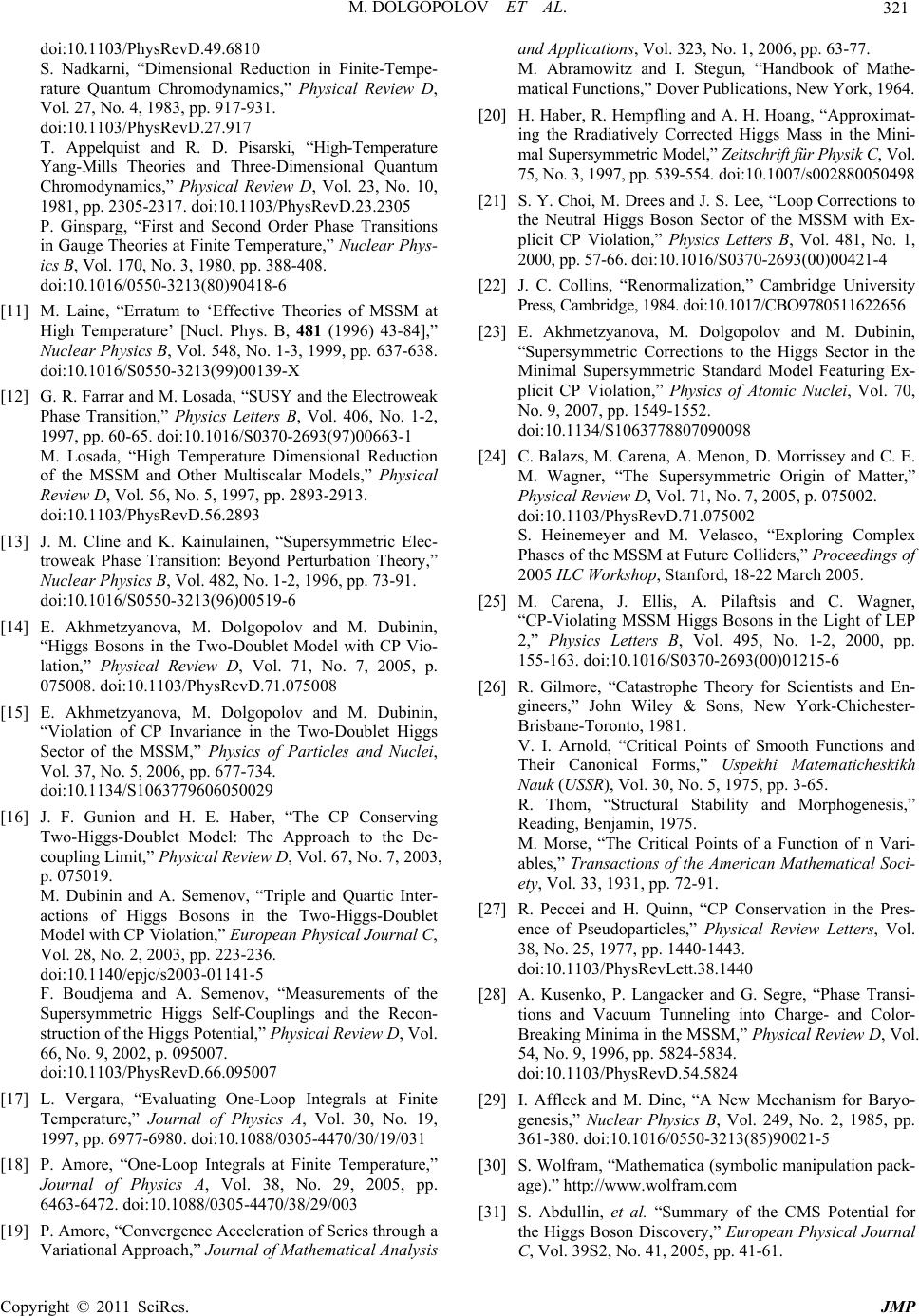 M. DOLGOPOLOV ET AL. Copyright © 2011 SciRes. JMP 321 doi:10.1103/PhysRevD.49.6810 S. Nadkarni, “Dimensional Reduction in Finite-Tempe- rature Quantum Chromodynamics,” Physical Review D, Vol. 27, No. 4, 1983, pp. 917-931. doi:10.1103/PhysRevD.27.917 T. Appelquist and R. D. Pisarski, “High-Temperature Yang-Mills Theories and Three-Dimensional Quantum Chromodynamics,” Physical Review D, Vol. 23, No. 10, 1981, pp. 2305-2317. doi:10.1103/PhysRevD.23.2305 P. Ginsparg, “First and Second Order Phase Transitions in Gauge Theories at Finite Temperature,” Nuclear Phys- ics B, Vol. 170, No. 3, 1980, pp. 388-408. doi:10.1016/0550-3213(80)90418-6 [11] M. Laine, “Erratum to ‘Effective Theories of MSSM at High Temperature’ [Nucl. Phys. B, 481 (1996) 43-84],” Nuclear Physics B, Vol. 548, No. 1-3, 1999, pp. 637-638. doi:10.1016/S0550-3213(99)00139-X [12] G. R. Farrar and M. Losada, “SUSY and the Electroweak Phase Transition,” Physics Letters B, Vol. 406, No. 1-2, 1997, pp. 60-65. doi:10.1016/S0370-2693(97)00663-1 M. Losada, “High Temperature Dimensional Reduction of the MSSM and Other Multiscalar Models,” Physical Review D, Vol. 56, No. 5, 1997, pp. 2893-2913. doi:10.1103/PhysRevD.56.2893 [13] J. M. Cline and K. Kainulainen, “Supersymmetric Elec- troweak Phase Transition: Beyond Perturbation Theory,” Nuclear Physics B, Vol. 482, No. 1-2, 1996, pp. 73-91. doi:10.1016/S0550-3213(96)00519-6 [14] E. Akhmetzyanova, M. Dolgopolov and M. Dubinin, “Higgs Bosons in the Two-Doublet Model with CP Vio- lation,” Physical Review D, Vol. 71, No. 7, 2005, p. 075008. doi:10.1103/PhysRevD.71.075008 [15] E. Akhmetzyanova, M. Dolgopolov and M. Dubinin, “Violation of CP Invariance in the Two-Doublet Higgs Sector of the MSSM,” Physics of Particles and Nuclei, Vol. 37, No. 5, 2006, pp. 677-734. doi:10.1134/S1063779606050029 [16] J. F. Gunion and H. E. Haber, “The CP Conserving Two-Higgs-Doublet Model: The Approach to the De- coupling Limit,” Physical Review D, Vol. 67, No. 7, 2003, p. 075019. M. Dubinin and A. Semenov, “Triple and Quartic Inter- actions of Higgs Bosons in the Two-Higgs-Doublet Model with CP Violation,” European Physical Journal C, Vol. 28, No. 2, 2003, pp. 223-236. doi:10.1140/epjc/s2003-01141-5 F. Boudjema and A. Semenov, “Measurements of the Supersymmetric Higgs Self-Couplings and the Recon- struction of the Higgs Potential,” Physical Review D, Vol. 66, No. 9, 2002, p. 095007. doi:10.1103/PhysRevD.66.095007 [17] L. Vergara, “Evaluating One-Loop Integrals at Finite Temperature,” Journal of Physics A, Vol. 30, No. 19, 1997, pp. 6977-6980. doi:10.1088/0305-4470/30/19/031 [18] P. Amore, “One-Loop Integrals at Finite Temperature,” Journal of Physics A, Vol. 38, No. 29, 2005, pp. 6463-6472. doi:10.1088/0305-4470/38/29/003 [19] P. Amore, “Convergence Acceleration of Series through a Variational Approach,” Journal of Mathematical Analysis and Applications, Vol. 323, No. 1, 2006, pp. 63-77. M. Abramowitz and I. Stegun, “Handbook of Mathe- matical Functions,” Dover Publications, New York, 1964. [20] H. Haber, R. Hempfling and A. H. Hoang, “Approximat- ing the Rradiatively Corrected Higgs Mass in the Mini- mal Supersymmetric Model,” Zeitschrift für Physik C, Vol. 75, No. 3, 1997, pp. 539-554. doi:10.1007/s002880050498 [21] S. Y. Choi, M. Drees and J. S. Lee, “Loop Corrections to the Neutral Higgs Boson Sector of the MSSM with Ex- plicit CP Violation,” Physics Letters B, Vol. 481, No. 1, 2000, pp. 57-66. doi:10.1016/S0370-2693(00)00421-4 [22] J. C. Collins, “Renormalization,” Cambridge University Press, Cambridge, 1984. doi:10.1017/CBO9780511622656 [23] E. Akhmetzyanova, M. Dolgopolov and M. Dubinin, “Supersymmetric Corrections to the Higgs Sector in the Minimal Supersymmetric Standard Model Featuring Ex- plicit CP Violation,” Physics of Atomic Nuclei, Vol. 70, No. 9, 2007, pp. 1549-1552. doi:10.1134/S1063778807090098 [24] C. Balazs, M. Carena, A. Menon, D. Morrissey and C. E. M. Wagner, “The Supersymmetric Origin of Matter,” Physical Review D, Vol. 71, No. 7, 2005, p. 075002. doi:10.1103/PhysRevD.71.075002 S. Heinemeyer and M. Velasco, “Exploring Complex Phases of the MSSM at Future Colliders,” Proceedings of 2005 ILC Workshop, Stanford, 18-22 March 2005. [25] M. Carena, J. Ellis, A. Pilaftsis and C. Wagner, “CP-Violating MSSM Higgs Bosons in the Light of LEP 2,” Physics Letters B, Vol. 495, No. 1-2, 2000, pp. 155-163. doi:10.1016/S0370-2693(00)01215-6 [26] R. Gilmore, “Catastrophe Theory for Scientists and En- gineers,” John Wiley & Sons, New York-Chichester- Brisbane-Toronto, 1981. V. I. Arnold, “Critical Points of Smooth Functions and Their Canonical Forms,” Uspekhi Matematicheskikh Nauk (USSR), Vol. 30, No. 5, 1975, pp. 3-65. R. Thom, “Structural Stability and Morphogenesis,” Reading, Benjamin, 1975. M. Morse, “The Critical Points of a Function of n Vari- ables,” Transactions of the American Mathematical Soci- ety, Vol. 33, 1931, pp. 72-91. [27] R. Peccei and H. Quinn, “CP Conservation in the Pres- ence of Pseudoparticles,” Physical Review Letters, Vol. 38, No. 25, 1977, pp. 1440-1443. doi:10.1103/PhysRevLett.38.1440 [28] A. Kusenko, P. Langacker and G. Segre, “Phase Transi- tions and Vacuum Tunneling into Charge- and Color- Breaking Minima in the MSSM,” Physical Review D, Vol. 54, No. 9, 1996, pp. 5824-5834. doi:10.1103/PhysRevD.54.5824 [29] I. Affleck and M. Dine, “A New Mechanism for Baryo- genesis,” Nuclear Physics B, Vol. 249, No. 2, 1985, pp. 361-380. doi:10.1016/0550-3213(85)90021-5 [30] S. Wolfram, “Mathematica (symbolic manipulation pack- age).” http://www.wolfram.com [31] S. Abdullin, et al. “Summary of the CMS Potential for the Higgs Boson Discovery,” European Physical Journal C, Vol. 39S2, No. 41, 2005, pp. 41-61.  M. DOLGOPOLOV ET AL. Copyright © 2011 SciRes. JMP 322 [32] H. Haber, R. Hempfling, “The Renormalization-Group Improved Higgs Sector of the Minimal Supersymmetric Model,” Physical Review D, Vol. 48, No. 9, 1993, pp. 4280-4309. doi:10.1103/PhysRevD.48.4280 Appendix Supersymmetric potential of the Higgs bosons - third generation of scalar quarks interaction has the form [32] 0, MQ VV VVV (82) where 22 2*2* , Mijij Q UD VMQQ MUUM DD (83) 2 ** ** 2, DUT iiii DU ii ii VQDiQU QD iQU (84) ** * 2 ( 1.., ,,,1,2, 2 jl ikijk l QUD i jijijij Q ij ij T ij ij V QQUU DD QQ iDUhcijkl (85) Q V denotes the four scalar quarks interaction terms, 2 0 0 i i , and are defined by the tree-level equalities 22222 2121 2222 22 22 2 11 11 diag ,, 44 11 diag,, 22 11 diag ,, 44 Q QUQ Q DU U UUU ggYh ggY hggh gYhgY 22 2 11 11 diag,, 44 . D DDD UD hgYgY hh Here the squark hypercharges are 131 i Q Y, i Y 232, 43 i U Y , and the Yukawa couplings for the third generation squarks 22 ,. sin cos tb tb mm hh vv In the general case of complex-valued parameters 1;2 1;2 ;, ;, UD UU DD hA hA (86)
|